The phase transition in random catalytic sets

Abstract

The notion of (auto) catalytic networks has become a cornerstone in understanding the possibility of a sudden dramatic increase of diversity in biological evolution as well as in the evolution of social and economical systems. Here we study catalytic random networks with respect to the final outcome diversity of products. We show that an analytical treatment of this longstanding problem is possible by mapping the problem onto a set of non-linear recurrence equations. The solution of these equations show a crucial dependence of the final number of products on the initial number of products and the density of catalytic production rules. For a fixed density of rules we can demonstrate the existence of a phase transition from a practically unpopulated regime to a fully populated and diverse one. The order parameter is the number of final products. We are able to further understand the origin of this phase transition as a crossover from one set of solutions from a quadratic equation to the other.

I Introduction

Chemicals act on chemicals to produce new chemicals, goods act on goods to produce new goods, ideas act on ideas to produce new ideas. The concept that elements of a set act on other elements of the same set to produce new elements which then become part of this set is ubiquitous not only in nature but also in social systems and processes. We might think of the development of modern chemistry, where the invention of a new compound leads to possibilities to use this compound (as a catalyst) to produce yet another compound. The same is true for economy, where one newly introduced good can be used as a tool to produce new goods and tools. Other famous example are recent models of evolution, maybe even our whole concept of history in general can be seen as a process of this type.

Maybe the most fascinating question associated with these processes is under which conditions self-sustaining systems can emerge, i.e. that the newly produced chemicals, goods, or ideas find adequate other new or old chemicals, goods, and ideas such that they can act on each other to produce yet new products, and so on. For any scientific approach to this subject it is clear that it is necessary to specify rules, which product can act on another product to produce a third one. For example there is a chemical rule that oxygen and hydrogen will produce water but there is no rule that gold and helium can form a compound. There is a rule that a hammer acting on a block of iron will produce sheet metal, but no rule that welding together two blocks of uranium 238 will lead to a big block of uranium. If one imagines that all existing and non-existing – but possible – products are listed in a high dimensional vector, than the rules how those elements can act on each other can be thought of elements in an interaction matrix, where a zero entry means no interaction, and a non-zero element gives the interaction strength.

In history there have been plenty of instances where a system of the above type underwent a transition from a state with very few products to a state of vast abundance of products. These transitions happen over relatively short timescales. An example from biology is the Cambrian explosion cambrium , where an unprecedented number of new taxa emerged within very short timescales. An economical example is the industrial revolution, where the number of industrial goods exploded to previously unimaginable numbers, a social example is the explosion of culture with the advent of the renaissance, or a more modern example the explosion of the number chemical compounds in the last century.

All of these ’explosive’ processes share the same structure: There are possibly constructively interacting elements, interaction is governed by a set of rules (natural laws, social consensus, religious restrictions), and a number of initially existing products. What does trigger the explosive event, why is this event sometimes missing for very long timeperiods? The only parameters at hand are: the number of rules, the number of initially present elements, and a possible structure in the interaction matrix. It is likely that the cultural explosion was driven by an increase of rules which was possible by driving back religious restrictions. The explosion of chemical compounds was possible by discovering the rules of modern chemistry. Let us mention here that for well studied systems the set of rules can in principle be known completely. However, for large systems, it might be wise as a first step to model them stochastically, i.e. let the interaction matrix be a random matrix. In this case there will of course be no structure in the interaction matrix, and the only parameters will be rule density $r$ and initial number $a_{0}$ of existing elements.

Since quite some time there has been conjectured the existence of a phase transition in the above systems, e.g. in farmer1 . By this we mean that in the $r-a_{0}$ plane there exist well defined regions,which are practically unpopulated, or almost fully populated, with a sharp transition between the regimes. This means that fixing the number of initial elements there exists a critical density of rules $r_{crit}$. When the system is below $r_{crit}$ the number of elements will remain relatively low compared to the total number of possible products. Above $r_{crit}$ the system will become self-sustaining and drive towards a heavyly populated state.

Even though this setting seems to be fundamental to a variety of disciplines, and its importance has long been noticed schumpeter11 ; order , the progress of a systematic scientific treatment of these problems is limited. Relevant contributions to this field come from chemistry and biology. The adequate mathematical treatment of such processes are so-called catalytic equations, which are sets of coupled, quadratic, ordinary differential equations. Special cases of those equations are for example the class of Lotka-Volterra replicators, the hypercycle eigen , or more recent ideas like the Turing gas fontana . Replicator dynamics, which is linear, is obtained from catalytic dynamics by a proper scaling of time. It is needless to mention that the non-linear catalytic equations carry tremendous potential of complex dynamics, however, in earlier studies some robustness in terms of fixed points seems to have been observed. For more details see stadler93 .

The aim of the present work is to prove the existence and study details of the nature of the above mentioned phase transition. This is possible by introducing some concepts of set theory, and – making use of the random structure of the production rules – by mapping the size of a consecutive series of sets into a set of update equations, which can be solved and analyzed. The analytic formulas give insights into what is happening at the transition. A practical aspect of this present work is that we cover analytically the large system limit, which is beyond numerical reachability, and has sofar not been possible to study.

The intuition for this work is based on a bit-string formulation of the above problem, which is a generalization of models recently termed random grammars order . In the bit-string model there is a set of initial bit-strings and a set of strings which act on these strings by either combining strings or substituting sub-strings. These latter strings can be seen as catalysts, their existence constitutes the presence of rules of what can be combined and/or substituted. The model which is presented below can be shown to be one to one compatible with the substitution and combination rules in the Kauffman bit-string model.

The paper is structured as follows: Section 2, where the hard working authors state the formal problem and develop the necessary notation and concepts. Section 3, where the brave authors derive the set of update equations. Section 4, where the struggling authors succeed in solving these equations reasonably well, and Section 5, where the victorious authors present their results. In Section 6 we discuss the results.

II The network-equation and some notation

Our basic concept is to view the abundances of all possible products as entries in a $d$-dimensional time-dependent vector $x(t)$, i.e. $x_{i}(t)$ is the quantity of product $i$ present at time $t$. We drop the time notation in the following. The population dynamics of a system, where product $i$ under the influence of product $j$ produces product $k$ is given by network-equations of the following type

$$\dot{x}_{k}=(x,\alpha^{k}x)-x_{k}\Phi\quad,\quad\Phi=\sum_{k}(x,\alpha^{k}x)\quad.$$ (1)

with $k\in\Lambda$, and the component $\alpha^{k}_{ij}>0$. $\Lambda$ is the domain of nodes – or put in fancier terms – the index set of the dynamic process. $(,)$ is the inner product of statevector $x$ with dimensionality $d=|\Lambda|$, the number of all possible products or nodes. The statevector is a vector of relative frequencies $0\leq x_{k}<1$, and $\sum_{k}x_{k}=1$. Each $\alpha^{k}$ is a linear operator providing the quadratic forms $(.,\alpha^{k}.)$ and encodes the structural information about which binary combinations $(i,j)\in\Lambda^{2}$, the substrates, can interact in order to form product $k$. Each entry in $\alpha^{k}$ is a real number, however, for the sake of simplicity we consider only 1 for interaction or 0 for no interaction. $\alpha^{k}$ can be thought of as the set of rules how objects interact. In the following $\alpha^{k}$ is sampled as a random matrix in the following way: We assume that for each product $k\in\Lambda$ there are pairs of substrate $(L(k),M(k))\in\Lambda^{2}$ such that $L(k)\stackrel{{\scriptstyle M(k)}}{{\longrightarrow}}\{k\}$. In words, this arrow means: $k$ is produced by substrate $L(k)$ under the ’influence’ of substrate $M(k)$. Note, that $L(k)$ and $M(k)$ do not have to be unique, there can be more than one pair $(L(k),M(k))$ producing a specific product $k$. Lets call the number of pairs leading to product $k$, ${\cal N}_{L,M}(k)$. We define the production rule density as the average number of pairs leading to one product

$$r/2=\langle{\cal N}_{L,M}(k)\rangle_{k}\quad.$$ (2)

Equations like (1) are long known for their rather surprising robustness in terms of fixed points where the system converges to. This is not obvious and one would rather expect a situation more dominated by more complicated orbits and limit cycles. For a more detailed discussion of this type of equations see stadler93 . Fixed points will therefore provide much information about the effective behavior of such systems, the fixed point equation being

$$x^{*}_{k}=\frac{1}{\Phi^{*}}(x^{*},\alpha^{k}x^{*})\quad.$$ (3)

We are dealing with a nonlinear process, so that the solutions of the network-equation will in general depend strongly on the initial conditions. Even assuming the process to be driven towards a stable fixed point does not imply the uniqueness of that fixed point.

II.1 Notation

We want to get some feeling what to expect when investigating the population dynamics of randomly sampled fixed 0/1-networks. The dynamical properties of Eq. (1) are linked to specific topologies. Knowing the topologic features will enable one to solve for the dynamics. Not knowing the interaction tensor $\alpha$ exactly, and only given its statistical properties, following the classical concept of statistical physics, one still can understand the expected dynamics of the system, and in particular its expected final outcome. We hence study the system in a probabilistic fashion, i.e. averaging over all possible topologies. The choices for $(L,M)(k)$ are equally distributed and $L$ and $M$ can be seen as independent random variables

The question we try to answer is: with how many products do we expect to end up with when starting from a given number of randomly choosen initial substrate species? Before we proceed we need a number of definitions. We denote the number of elements contained in some set $A$ by writing $|A|$, and define the support of a process at a given time

$$S(x):=\left\{k|x_{k}>0\right\}\quad.$$ (4)

Suppose that the process is driven to a (stable) fixed point such that the final support is

$$S^{*}(x):=S(\lim\limits_{t\rightarrow\infty}x(t))\quad.$$ (5)

Inversely, we can ask which initial conditions end up in the same fixed point and define the body of this fixed point to be the set

$$B(x^{*}):=\left\{x|\sum_{k}x_{k}=1\wedge\lim\limits_{t\rightarrow\infty}x(t)=x^{*}\right\}\quad.$$ (6)

We further define the following operations on product-sets: the foreward difference of set $A$,

$$\partial_{+}A:=\left\{k\in\Lambda|\{L(k),M(k)\}\subset A\right\}\setminus A$$ (7)

and the backward difference of $A$,

$$\partial_{-}A:=\cup_{k\in A}\{L(k),M(k)\}\setminus A\quad.$$ (8)

With these operations we can define the foreward closure of set $A$

$$\bar{A}^{+}:=\cap\left\{B|A\subset B\wedge\partial_{+}B\subset B\right\}\quad,$$ (9)

and the backward closure of a set,

$$\bar{A}^{-}:=\cap\left\{B|A\subset B\wedge\partial_{-}B\subset B\right\}\quad.$$ (10)

These definitions can best be understood by viewing our dynamical system Eq. (1) as a directed graph whose nodes are connected by arrows. A node looking at its edges can therefore distinguish between feather ends or arrow heads. A node holding a feather end of an arrow is a substrate, a node holding an arrow head is a product with respect to this edge. Given some set of nodes we can identify for each node $k$ all the nodes which will be formed due to the influence of $k$ in the next timestep. In this sense we say the nodes look ’foreward’. The foreward difference of some set is therefore the set of all products the nodes of the set look foreward to, excluded the products that are already present as nodes of the set we started out with. The backward difference follows the same idea only looking at the arrows from arrowhead towards the feathers. The corresponding closures are then simply obtained by adding the set-differences iteratively to the initial set, i.e. we add the difference to the initial set and form a new difference on the first extension of the set, then add this difference to obtain the second extension of the initial set and so on, until the difference (forward or backward) is empty and the iterative process comes to a halt. That this eventually may happen can be understood by looking at chains of arrows as an example. Take a node and add an arrow pointing at some other randomly chosen node in the set. In the beginning the chance to select a virginal node is high and the chain will grow but as the chain grows the probability of sampling a member already in the chain increases, and even though the single sample probability may still be small, the chance to sample into the chain eventually is not.

For clarity let us summarize our philosophy: All objects which can possibly act on each other are represented by the index set $\Lambda$ of the processing system Eq. (1), which contains all the ’names’ of the considered and ’thinkable’ objects. The index set provides the domain for all dynamical considerations. Properties of the system are implemented via the map $x:\Lambda\rightarrow{\bf R}_{+}$, which are the relative frequencies of the indexed species in the domain. We are not interested in particular weights but only in the directed network topology coded by the matrices $\alpha^{k}$ on the domain $\Lambda$. Not only does this topological approach provide us with the means to talk about randomly distributed productive substrate pairs, but also about their density of occurrence $r$. Even more important, if we are not interested in details of the dynamics but decide to focus only on how large the expected final set will be (given some initial substrate set and density) we can drop dynamical considerations and pass to topological ones. We are not interested in how much of each object species we will effectively end up with, just if it got produced or not. The subset of the domain that is effectively populated is called the support $S\subset\Lambda$. To investigate the flow of the support under the network equation we may utilize set-operations compatible with the topological structure of directed reaction graphs leading to the definition of the forward and the backward difference and their respective closures. It is intuitively clear, that the forward closure of some set is the subset of the domain that is flooded by the initial set during the production process. It necessarily forms an upper limit for the size of possible self-sustainable subsets of the domain reachable from the initial condition. In a simplification considering an equally distributed random interaction topology we gain a notion of expected growth rates for the set-differences based on expected sampling rates. This leads to equations of expected growth as demonstrated next.

III The growth laws for catalytic sets

We now develop a method to compute the size of the foreward closure $a_{\infty}=|\bar{A}^{+}|$ as a function of the production rule density and the size of the initial set $A$. $a_{\infty}$ is the final number of products once the system has converged. The probability of some fixed $k$ being the product of some fixed pair of substrates, $l$ and $m$ is obviously

$$p=\frac{2}{d(d-1)}\quad.$$ (11)

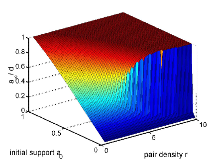
(a)

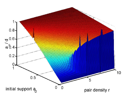
(b)

Figure 1: Solution to the update equations Eq. (15) (a) and its analytical approximation Eq. (22) (b). There is clearly a critical line in the $r-a_{0}$ plane where a transition from an unpopulated to an almost fully populated regime occurs. The spikes in (b) are due to numerical problems in the plot with poles in the solution $a_{\infty}$.

Imagine an initial random set $A_{0}$ of products with a number of $a_{0}=|A_{0}|$ elements. Given the dimensionality $d$ of the system and a production rule density $r$, the expected number of produced elements in the next timestep is the number of possible pairs in $A_{0}$ times the probability to find a productive pair, i.e.

$$\frac{rd}{2}\left(\begin{array}[]{c}a\\ 2\end{array}\right)p=\frac{ra(a-1)}{2(d-1)}\sim\frac{ra^{2}}{2d}\quad.$$ (12)

Several of these newly created elements will already be $\in A_{0}$. The probability that one of these produced elements is not yet $\in A_{0}$ is $1-a_{0}/d$, leading to the actual size of the catalytic set at time 1, $A_{1}$

$$a_{1}=a_{0}+\Delta a_{0}\quad{\rm with}\quad\Delta a_{0}=\frac{r}{2d}\left(1-\frac{a_{0}}{d}\right)a_{0}^{2}\quad,$$ (13)

with $\Delta a_{0}=|\partial_{+}A_{0}|$ being the increment of elements. What will happen in the next timestep? We now have $A_{1}=A_{0}\cup\partial_{+}A_{0}$. The increment for the next timestep will be made up of all the new products which are possible (and not already in $A_{1}$) by combining two elements from $\partial_{+}A_{0}$, or by combining one element from $\partial_{+}A_{0}$ with one from $A_{0}$. The number of possible pairs for those combinations are $\Delta a_{0}(\Delta a_{0}-1)/2\sim\Delta a_{0}^{2}/2$ and $a_{0}\Delta a_{0}$, respectively. Note, that the third possibility combining 2 elements from the set $A_{0}$ will always lead to $\partial_{+}A_{0}$ which is already $\in A_{1}$, and no new products can emerge from this. These possibilities multiplied by $p$, $rd/2$ and probability that the new product lies in $A_{1}$ already, lead to the increment for the second timestep

$$\Delta a_{1}=\frac{r}{2d}\left(1-\frac{a_{1}}{d}\right)\left(\Delta a_{0}^{2}+2a_{0}\Delta a_{0}\right)$$

$$=\frac{r}{2d}\left(1-\frac{a_{1}}{d}\right)\left(a_{1}^{2}-a_{0}^{2}\right)\quad.$$ (14)

Now continue the iterative sceme $A_{t+1}=A_{t}\cup\partial_{+}A_{t}$. This means that the set at time $t+1$ is the old set plus the products newly generated in the timespan $[t,t+1]$. We can finally write down a growth equation for catalytic sets

$$a_{t+1}=a_{t}+\Delta a_{t}\,\,,\,\,\Delta a_{t+1}=\frac{r}{2d}\left(1-\frac{a_{t+1}}{d}\right)\left(a_{t+1}^{2}-a_{t}^{2}\right)\,\,,$$ (15)

with initial conditions $a_{0}=|A_{0}|$ and $a_{-1}=0$. To sum up, we have to take care of all possible new pairs by looking at all new elements added in an iteration step and the new pairs they can build with themselves. We also have to take into account all the pairs they can build with elements produced earlier. We have to exclude all the pairs that allready have been considered. This is all captured by Eq. (15), which should be noted to be scale invariant with respect to dimension $d$. To see this just scale $a\longrightarrow a/d$, and the dimension drops out of the equation. It is therefore fully justified to drop $d$ from Eq. (15), if wanted.

IV Solution of the update equation - Result

The solution of the growth equation Eq. (15) with respect to the productive pair density $r$ and the initial set-size $a_{0}$ is given in Fig. 1 (a). The immediate message is that there is a critical density $r_{crit}$ above which a continuous increase of the initial set-size $a_{0}$ does not correspond with a continuous increase of its foreward closure size $a_{\infty}$, but displays a phase transition, a jump from small to very large foreward closures at some $a_{0}^{crit}(r)$. $a_{0}^{crit}$ vanishes for $r<r_{crit}$. This demonstrates unambiguously the existence of a phase transition in catalytic random systems.

IV.1 Analytical approximation of the foreward closure size

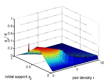
(a)

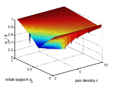
(b)

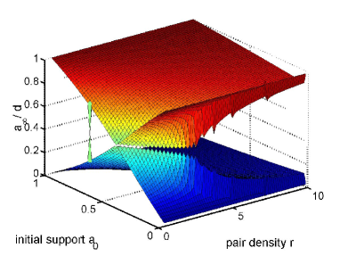
(c)

Figure 2: Plot of the solutions $a_{\infty-}$ (a), $a_{\infty+}$ (b) and both of the above in one plot (c). It is clear that the pase transition happens as the solutions switch from $a_{\infty+}$ to $a_{\infty-}$.

Let us define $c_{t}=\Delta a_{t+1}/\Delta a_{t}$. As an approximation imagine for a moment that $c_{t}$ is a constant in time $c$. Then for the forward closure

$$a_{\infty}=\sum_{t}c^{t}a_{0}=\frac{1}{1-c}\quad.$$ (16)

A choice $c$ which produces the right asymptotical results is

$$c=r\left(1-\frac{a_{\infty}}{d}\right)\frac{a_{\infty}}{d}\quad,$$ (17)

which is seen by first dividing the right part of Eq. (15) by $\Delta a_{t}$ and then taking the $t\longrightarrow\infty$ limit. Now use the Ansatz

$$a_{\infty}=\frac{a}{1-c}\quad,\quad c=r\left(1-\frac{a_{\infty}}{d}\right)\frac{a_{\infty}}{d}\quad,$$ (18)

which leads to a polynomial of third degree $a_{\infty}^{3}-a_{\infty}^{2}d+a_{\infty}\frac{d^{2}}{r}-\lambda a\frac{d^{2}}{r}=0$, or in terms of $c$

$$c^{3}-2c^{2}+c(1+r\frac{a}{d})+r\frac{a}{d}\left(\frac{a}{d}-1\right)=0\quad.$$ (19)

Substituting $c=x+2/3$ reduces to equation $x^{3}+px+q=0$ with

$$p=-\frac{1}{3}\left(1-3r\frac{a}{d}\right)\qquad q=\frac{2}{27}+\frac{1}{3}r\frac{a}{d}\left(3\frac{a}{d}-1\right)\quad,$$ (20)

so that Cardano’s method can be used with $x=y+z$ to get

$$y=\left[-\frac{q}{2}+\sqrt{(q/2)^{2}+(p/3)^{3}}\right]^{\frac{1}{3}}\qquad z=-\frac{p}{3y}\quad,$$ (21)

providing us with three solutions $y+z$, $\rho^{2}y+\rho z$ and $\rho y+\rho^{2}z$ with $\rho=\exp(2\pi i/3)$. We are only interested in the real solution $y+z$ which yields the final result

$$a_{\infty}=\frac{a}{1-c}\quad{\rm with}\quad c=2/3+y+z\quad,$$ (22)

which is a good approximation of the true solution of the forward equation Eq. (15) and is plotted in Fig. 1 (b) in the $a_{0}$–$r$ plane. The comparison with Fig. 1 (a) demonstrates the quality of the analytical solution.

The analytical form of the solution allows us to understand the origin of the phase transition. For this reason we observe that we can compute $a_{\infty}$ by solving $c=r(1-a_{\infty})a_{\infty}$ providing us with two solutions

$$a_{\infty\,\pm}=\frac{d}{2}\left(1\pm\sqrt{1-4\frac{c}{r}}\right)\quad.$$ (23)

These solutions are shown in Figs. 2 (a) and (b). It becomes obvious that the phase transition actually always takes place by the system switching from the one solution to the other at $a_{0}^{crit}(r)$. Below a critical value of $r_{crit}$ the one solution smoothely passes into the other. We observe a crossover of the probable and the improbable solution. Most likely this is due to a convexity argument, implying the monotonicity of the size of the forward closure with respect to the size of the initial condition. The size of the forward closure will not shrink with increasing the initial set size and therefore has to jump to the alternative solution at some critical line. As long as the third order polynomial is strictly monotonic we have a unique real solution for the zero of the polynomial. At $r_{crit}$ the polynomial starts to have a local minimum and maximum and we have in fact two relevant real zeros (out of three), the large and the small solution. $r_{crit}$ is determined by the tripple zero of the polynomial. Note a famous analogy here: Just as in the Vanderwaal’s gas we can draw Maxwell lines. At the phase-transition, the small solution becomes instable, the large solution becomes stable. Here the productive pair density $r$ takes the role of temperature in the Vanderwaal’s gas. Below the critical value a system freezes into a small set of durable species, while above the critical production law density, supercritical but yet small sets of individuals evaporate into their foreward closure. The difference we have here compared to Vanderwaal’s gas is that the liquid phase is concentrated on the high edge of the phase transition, while the phase-plane itself is a solid-liquid mixture.

V Discussion and outlook

We have developed a way to map a conceptual system of autocatalytic agents into a quantitative framework. With this it is possible to show that the combination of the initial number of products $a_{0}$ and the density of mutual production rules $r$ is crucially influencing the mode of growth of sets of products. Our main result is that we were able to map the class of random catalytic networks into a set of growth equations, which allows us to study the expectation value of the final number of products. The resulting equation can be solved and shows a clear phase transition from practically unpopulated zones towords almost fully populated ones, in ’rule density–initial number of products’ space. The transition is a crossover between two sets of solutions to a quadratic equation.

We believe that this nicely resembles numerical-experimental findings of stadler93 , where the authors find a decrease of species with an increase of $p_{el}$ in their Fig. 1 (d). The fact that the transition from small to full forward closure sizes is gradual, is either due to the limited system size (10 species), or that the initial support was high, i.e. above $a_{0}^{crit}(r)$, so that no sharp increase could be found. In fact, systems of the type of Eq. (1) are straight forwardly solvable numerically up to system sizes of about $d=100$ within reasonable computing time. We note that the practical value of this present work is that it captures the large system size limit, which is out of numerical reach and was not tractable analytically before.

The present approach does not try to explain the detailed role of auto catalytic cycles nor of keynode species in the context of understanding the beginning of an explosion of species numbers as was very nicely done for example in jain99 ; jain02 . The periods of fast extinction reported there are not incorporated in our consideration yet, since we have not taken any evolutionatry hypotheses into account so far, nor did we incorporate evolutionary concepts in the sense that products are associated characteristics (some sort of fitness, e.g. the weight $x_{k}$) upon which they can get selected by some method. Taking these arguments into account seems a natural starting point for future research. We believe that it should be possible that a combination of backward and forward closure arguments can be used to estimate a critical density of auta catalytic cycles necessary for a system to become critical as studied here. We have not so-far considered negative entries in the interaction matrices, which should also be present in natural or social systems. Finally, we mention that our arguments given here should – due to the absence of a characteristic scale in the update equations – not be limited to finite sets.

Acknowledgments: S.T. would like to thank the SFI and in particular J.D. Farmer for their great hospitality and support in Sept-Oct of 2004. The project was funded in part by the Austrian Council, and FWF project P17621 G05.

References

- (1) S.J. Gould, (1989) Wonderful Life (Harvard University Press, Cambridge Mass., 1989).
- (2) J.D Farmer, S.A. Kauffman, N.H. Packard, Physica D 22 50-67 (1986).
- (3) J.A. Schumpeter, Theorie der wirtschaftlichen Entwicklung (Wien, 1911).
- (4) S.A. Kauffman, The Origins of Order, (Oxford University Press, London, 1993).
- (5) M. Eigen, P. Schuster, The Hypercycle (Springer Verlag, Berlin, 1979).
- (6) W. Fontana, in Articial Life II, C.G. Langton, C. Taylor, J.D. Farmer, S. Rasmussen, eds. (Addison-Wesley, Redwood City CA), pp. 159-210 (1992).
- (7) P.F. Stadler, W. Fontana, J.H. Miller, Physica D 63, 378-392 (1993).
- (8) S. Jain, S. Krishna, Phys. Rev. Lett. 81, 5684-5687 (1998).
- (9) S. Jain, S. Krishna, Proc. Natl. Acad. Sci. USA 99, 2055-2060 (2002).