Quantum kinetic description of Coulomb effects
in one-dimensional nano-transistors

Abstract

In this article, we combine the modified electrostatics of a one-dimensional transistor structure with a quantum kinetic formulation of Coulomb interaction and nonequilibrium transport. A multi-configurational self-consistent Green’s function approach is presented, accounting for fluctuating electron numbers. On this basis we provide a theory for the simulation of electronic transport and quantum charging effects in nano-transistors, such as gated carbon nanotube and whisker devices and one-dimensional CMOS transistors. Single-electron charging effects arise naturally as a consequence of the Coulomb repulsion within the channel.

I Introduction

As scaling of field-effect-transistor (FET) devices reaches the deca-nanometer regime, multi-gate architectures and ultrathin active channel regions are mandatory in order to preserve electrostatic integrity. It has been shown that a coaxially gated nanowire represents the ideal device structure for ultimately scaled FETs.Auth and Plummer (1997); Wong (2002) A variety of 1D nanostructures - such as carbon nanotubes, silicon nanowires or compound semiconductor nano-whiskers - have been demonstrated and intensive research has been devoted to the realization of field-effect-transistor action in these nanostructures.Javey et al. (2004); Lin et al. (2005); McAlpine et al. (2003); Thelander et al. (2003) Due to the small lateral extent in the nanometer range, electronic transport through such nanowires is one-dimensional with only a few or even a single transverse mode participating in the current. As a result, increasingly less electrons are involved in the switching of a nanowire transistor. In fact, even in devices with rather long channel lengths of 100nm, only on the order of 1-10 electrons constitute the charge in the channel for on-state voltage conditions. Hence, single-electron charging effects are increasingly important and have to be taken into account.Yoneya et al. (2001); Suzuki et al. (2002); Amlani et al. (2003)

Two different approaches are commonly used to describe electronic transport in nano-transistors: A quantum kinetic approach based on real-time Green’s functions provides an excellent description of non-equilibrium states. Lake et al. (1997); Yongqiang et al. (2002, 2001) Here, the Coulomb interaction is described in terms of a selfconsistent Hartree potential, optionally combined with a spin-density-functional exchange-correlation term in local density approximation (LDA-SDFT). However, this framework does not account for single-electron charging effects without forcing integer electron numbers. Alternatively, the second approach considers a quasi-isolated nanosystem with a many-body formulation of Coulomb interaction, including electronic transport on a basis of rate-equations. Beenakker (1991); Averin et al. (1991); Jovanovic and Leburton (1993); Weimann et al. (1995); Tanaka and Akera (1996); Pfannkuche and Ulloa (1995); Indlekofer and Lüth (2000) While predicting single-electron charging effects correctly, the latter neglects dissipation and renormalization effects due to the source and drain contacts.

Here, we present a novel approach that allows to combine a quantum kinetic description of non-equilibrium electron transport with non-local many-body Coulomb effects in one-dimensional FET nanodevices. Within our approach, single-electron charging effects arise naturally as a consequence of the Coulomb interaction. Our formalism contains two central ingredients: In order to cope with particle-number fluctuations under nonequilibrium conditions, we introduce a multi-configurational self-consistent Green’s function algorithm. Secondly, we consider a one-dimensional Coulomb Green’s function for the transistor channel that allows to properly incorporate many-body interaction effects into a quantum kinetic approach with electrostatic boundary conditions for a realistic FET. As an example, we calculate the transfer characteristics of a nanowire transistor with Schottky-barriers (SB) at the contact-channel interfaces.

II Coulomb Green’s function

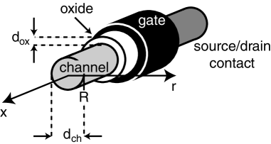
Figure 1: Schematic view of a 1D FET geometry. ($d_{ox}$ and $d_{ch}$ denote the gate insulator thickness and the channel diameter of the nano-transistor, respectively.)

Consider a coaxially gated field-effect-transistor as illustrated in Fig. 1. A cylindrical semiconducting channel material is surrounded by a thin dielectric and a metallic gate electrode. The electrostatic potential $V$ inside such a one-dimensional (1D) transistor channel obeys a modified Poisson equation Auth and Plummer (1997); Pikus and Likharev (1997)

$$\frac{\partial^{2}}{\partial x^{2}}V(x)-\frac{1}{\lambda^{2}}V(x)=-\frac{1}{\epsilon_{0}\epsilon_{ch}S}\rho(x)-\frac{1}{\lambda^{2}}V_{G},$$ (1)

where $\rho$ is the 1D charge density. $V_{G}$ denotes the gate potential and $S=\pi d^{2}_{ch}/4$ is the effective cross-sectional area. The characteristic length $\lambda$ is related to the spatial separation of the gate electrode from the channel (which should be smaller than the total length $L$ of the channel).Auth and Plummer (1997); Pikus and Likharev (1997) Note that Eq. (1) is an appropriate description for coaxial as well as planar transistor geometries, differing only in the characteristic length $\lambda$. In the following, we assume perfect metallic source and drain contacts at the boundaries, yielding fixed-potential boundary conditions due to given chemical potentials within these contacts.

A key ingredient in our formalism is the usage of a Coulomb Green’s function for the description of charge interaction within the channel. This allows us to formulate classical electrostatics (with boundary conditions) and many-body interaction between electrons on equal footing. The corresponding Coulomb Green’s function of the gated channel (with $0\leq x,x^{\prime}\leq L$ and vanishing potential at the boundaries $0,L$) can readily be obtained as

$$v(x,x^{\prime}) = \frac{\lambda}{2}\left(e^{-\frac{|x-x^{\prime}|}{\lambda}}-e^{-\frac{x+x^{\prime}}{\lambda}}\right)$$

$$+\frac{\lambda}{2}~{}e^{-\frac{L}{\lambda}}\left(\frac{\cosh\left(\frac{x-x^{\prime}}{\lambda}\right)}{\sinh\left(\frac{L}{\lambda}\right)}-\frac{\cosh\left(\frac{x+x^{\prime}}{\lambda}\right)}{\sinh\left(\frac{L}{\lambda}\right)}\right).$$

(In contrast, if we considered open boundary conditions, we would obtain $v(x,x^{\prime})=(\lambda/2)\exp\left(-|x-x^{\prime}|/\lambda\right)$ instead.) For a given charge density $\rho$ inside the channel, the potential thus reads

$$V(x)=\frac{1}{\epsilon_{0}\epsilon_{ch}S}\!\int\!\!dx^{\prime}~{}v(x,x^{\prime})~{}\rho(x^{\prime})+V_{ext}(x),$$ (3)

with the external potential contribution

$$V_{ext}(x) = \frac{\sinh\left(\frac{L-x}{\lambda}\right)}{\sinh\left(\frac{L}{\lambda}\right)}V_{S}+\frac{\sinh\left(\frac{x}{\lambda}\right)}{\sinh\left(\frac{L}{\lambda}\right)}V_{D}$$

$$+\frac{1}{\lambda^{2}}\!\int\!\!dx^{\prime}~{}v(x,x^{\prime})~{}V_{G},$$

where $V_{S}$ and $V_{D}$ denote the contact potentials.

III System Hamiltonian

In this article, we make use of a tight-binding description of the system, represented by a localized 1D single-particle basis $\{\phi_{j}(x,\sigma)\}$ (where the single-particle index $j$ represents a combined orbital, site, and spin multi-index.) The total system Hamiltonian $H=H_{0}+H_{ee}+H_{S}+H_{D}$ can be split into four parts. $H_{0}$ contains all single-particle terms of the transistor channel:

$$H_{0} = \sum_{i,j}h_{jk}~{}c^{\dagger}_{j}c_{k},$$ (5)

$$h_{jk} = -e\sum_{\sigma}\!\!\int\!\!dx~{}\phi^{*}_{j}(x,\sigma)~{}\phi_{k}(x,\sigma)\Big{[}V_{dop}(x)+V_{ext}(x)\Big{]}$$

$$+\delta_{jk}d_{j}+t_{jk},$$

with the electron annihilation operator $c_{j}$ for state $j$. The composition of the channel (material-specific properties, layer sequence, etc.) is described by $d_{j}$ and off-diagonal hopping matrix elements $t_{jk}$.Vogl et al. (1983); Støvneng and Lipavský (1994) $V_{dop}$ denotes the potential resulting from fixed charges $\rho_{dop}$ (due to ionized doping atoms), whereas $V_{ext}$ stems from external charges due to the applied drain-source voltage and the gate influence (see Eq. (II)).

Furthermore, $H_{S}$ and $H_{D}$ are the Hamiltonians for the source and drain contacts, respectively. Latter also contain the corresponding hopping terms to the outer ends of the channel region, providing electron injection and absorption. Each contact is assumed to be in a state of local equilibrium with an individual chemical potential according to the applied voltage. (See also Eqs. (9), (12) below.)

Most importantly, $H_{ee}$ describes the many-body Coulomb interaction between electrons within the channel region:Indlekofer and Lüth (2000)

$$H_{ee}=\frac{1}{2}\sum_{i,j,k,l}V_{mjkl}~{}c^{\dagger}_{m}c^{\dagger}_{j}c_{k}c_{l},$$ (6)

with Coulomb matrix elements

$$V_{mjkl} = \frac{e^{2}}{\epsilon_{0}\epsilon_{ch}S}\sum_{\sigma,\sigma^{\prime}}\int\!\!dx\!\!\int\!\!dx^{\prime}~{}v(x,x^{\prime})$$

$$\times~{}\phi^{*}_{m}(x,\sigma)~{}\phi^{*}_{j}(x^{\prime}\!,\sigma^{\prime})~{}\phi_{k}(x^{\prime}\!,\sigma^{\prime})~{}\phi_{l}(x,\sigma),$$

which employ the Coulomb Green’s function Eq. (II).

IV Quantum kinetics

A quantum kinetic description of the system (under nonequilibrium conditions in particular) is obtained via the usage of a real-time Green’s functions formalism.Schäfer and Wegener (2002); Haug and Jauho (1998); Datta (1995) The retarded and lesser (two-point) Green’s functions in the time domain are given by

$$G^{r}_{jk}(t) = -i\Theta(t)\langle\big{\{}c_{j}(t),c^{\dagger}_{k}(0)\big{\}}\rangle,$$ (8)

$$G^{<}_{jk}(t) = i\langle c^{\dagger}_{k}(0)c_{j}(t)\rangle,$$

for steady-state conditions. In the following, we will consider the Fourier transformed functions, defined via $G(E)=(1/\hbar)\!\int\!\!dt\exp(iEt/\hbar)G(t)$.

For temperatures $T$ well above the Kondo temperature of the system, the Coulomb interaction can be treated independently of the contact coupling, albeit self-consistently. In matrix notation, the Dyson equation for the channel thus can be written as Datta (1995); Henrickson et al. (1994); Lake et al. (1997)

$$G^{r} = G^{r0}+G^{r0}\left[\Sigma^{r}_{ee}+\Sigma^{r}_{S}+\Sigma^{r}_{D}\right]G^{r},$$ (9)

$$G^{<} = i~{}f_{0}~{}A$$

$$+i~{}(f_{S}-f_{0})~{}G^{r}\Gamma_{S}G^{a}$$

$$+i~{}(f_{D}-f_{0})~{}G^{r}\Gamma_{D}G^{a},$$

with $\Gamma_{S}\equiv i(\Sigma^{r}_{S}-\Sigma^{a}_{S})$, $\Gamma_{D}\equiv i(\Sigma^{r}_{D}-\Sigma^{a}_{D})$ and $A\equiv i(G^{r}-G^{a})$. $f_{S}$ and $f_{D}$ are the local source and drain Fermi distribution functions, respectively, assuming local equilibrium within these reservoirs. On the other hand, $f_{0}$ denotes the equilibrium distribution function of the isolated channel system (typically, $f_{0}=f_{D}$). Furthermore, $G^{r0}\equiv(E-h+i\epsilon)^{-1}$ (with $\epsilon\to 0+$) and $G^{a}={G^{r}}^{\dagger}$.

Once $G^{<}$ has been obtained selfconsistently from Eq. (9), observables like the electron density $\rho_{e}$ and the current $I_{e}$ (through an arbitrary layer at $x_{0}$) can be calculated via

$$\rho_{e}(x,\sigma) = -e\sum_{jk}~{}\phi^{*}_{j}(x,\sigma)~{}\phi_{k}(x,\sigma)~{}\hat{\rho}_{jk},$$ (10)

$$I_{e} = -\frac{e}{\hbar}\!\!\!\sum_{j,k\atop{x_{j}\leq x_{0},\atop x_{k}>x_{0}}}\!\!\!2~{}Im\left(t_{jk}~{}\hat{\rho}_{jk}\right),$$

with the single-particle density-matrix

$$\hat{\rho}_{jk}=\frac{1}{2\pi}\!\!\int\!\!dE~{}\frac{1}{i}G^{<}_{kj}(E).$$ (11)

The effective contact selfenergies due to the coupling of the channel to the source and drain regions ($c=S,D$) can be obtained as Henrickson et al. (1994); Indlekofer et al. (1996); Lake et al. (1997)

$${\Sigma^{r}_{c}}_{jk}(E)=\sum_{p,q\in c}{t_{c}}_{jp}~{}{G^{r0}_{c}}_{\!\!\!pq}(E)~{}{t_{c}}_{qk},$$ (12)

with the isolated contact Green’s function $G^{r0}_{c}$ and contact-channel hopping terms $t_{c}$.

The evaluation of the Coulomb selfenergy $\Sigma^{r}_{ee}$ requires a suitable approximation scheme due to the infinite Green’s function hierarchy (which is a consequence of the two-particle interaction). As a first-order expansion (Hartree-Fock diagrams), four-point Green’s functions can be factorized into linear combinations of products of two-point functions.Henrickson et al. (1994); Schäfer and Wegener (2002) Using this approximation, the Coulomb selfenergy reads

$${\Sigma^{r}_{ee}}_{ml}=\sum_{j,k}\left(V_{mjkl}-V_{jmkl}\right)\hat{\rho}_{jk}.$$ (13)

Note that $\Sigma^{<}_{ee}=0$, and $\Sigma^{r}_{ee}$ is non-local, hermitian and energy-independent (static) within the considered approximation scheme; compare also with Ref. Henrickson et al., 1994. For convenience, the Hartree potential (first $V$ term in Eq. (13))

$$V_{H}(x)=\frac{1}{\epsilon_{0}\epsilon_{ch}S}\sum_{\sigma^{\prime}}\int\!\!dx^{\prime}~{}v(x,x^{\prime})~{}\rho_{e}(x^{\prime}\!,\sigma^{\prime})$$ (14)

can be separated from the retarded Coulomb selfenergy (compare Eq. (3)), where the electron charge density $\rho_{e}$ is given by Eq. (10). Hence, the total electrostatic potential of the system reads $V=V_{dop}+V_{H}+V_{ext}$.

For integer-number electron filling conditions, Eq. (13) provides an excellent description of the system for application-relevant temperatures. However, under nonequilibrium conditions, one has to deal with non-integer average filling situations, which are beyond the scope of a first-order (mean-field) selfenergy in general. In the following section, we will therefore present a multi-configurational approach which is able to cope with such particle-number fluctuations.

V Multi-configurational self-consistent Green’s function

A thermodynamic state of the transistor channel with fluctuating electron number can be considered as a weighted mixture of many-body states with integer filling (configurations) of relevant single-particle states. For a given $G^{<}$, relevant single-particle states are defined as eigenstates of $\hat{\rho}$ (Eq. (11)) that exhibit significant occupation fluctuations and have a sufficiently small dephasing (due to the contact-coupling). This projection to a relevant single-particle subspace of dimension $N$ reduces the resulting Fock subspace dimension $2^{N}$ significantly, rendering this approach numerically feasible.

For each configuration, the Coulomb selfenergy approximation Eq. (13) becomes adequate. Then the Green’s function can be written as a configuration-average:

$$\bar{G}=\sum_{\kappa}w_{\kappa}~{}G[\hat{\rho}_{\kappa}],$$ (15)

where $\hat{\rho}_{\kappa}$ denotes the single-particle density-matrix (derived from $\hat{\rho}$) for configuration $\kappa$ with weight $w_{\kappa}$. $G[\hat{\rho}_{\kappa}]$ is the corresponding Green’s function (retarded and lesser) which is obtained by using Eqs. (9), (13).

The weight vector $w$ defines a projected nonequilibrium many-body statistical operator in the relevant Fock basis. (Note that the configurations defined above might not be exact eigenstates of the projected many-body Hamiltonian, containing Eq. (6) in particular. In the following, we restrict ourselves to the dominant diagonal elements of the many-body Hamiltonian in the relevant Fock basis.) Consequentely, the resulting many-body lesser Green’s function reads

$${G^{<}_{MB}[w]}_{jk}(t) = i~{}\sum_{\kappa,\lambda}w_{\kappa}~{}e^{\frac{i}{\hbar}(E_{\lambda}-E_{\kappa})t}$$

$$\times~{}\langle\kappa|c^{\dagger}_{k}|\lambda\rangle~{}\langle\lambda|c_{j}|\kappa\rangle,$$

where $|\kappa\rangle$ denotes a relevant Fock state with energy $E_{\kappa}$. In principle, $w$ must be chosen such that $\Delta(G^{<}_{MB}[w],G^{<})=\text{min}$ for a given $G^{<}$ within the relevant subspace, where $\Delta$ measures the cumulative difference of spectral weights of corresponding resonances. However, for most applications it is sufficient to consider a vector $w$ that maximizes the entropy at an effective temperature $T^{*}(T,V_{G},V_{D})$ under the (weaker) subsidiary condition that $\hat{\rho}_{MB}[w]=\hat{\rho}$ within the relevant subspace, where $\hat{\rho}_{MB}[w]$ denotes the many-body result.Indlekofer and Lüth (2000); Indlekofer et al. (2002, 2003) (Under moderate bias conditions, it is justified to assume $T^{*}\approx T$.)

In turn, $\bar{G}^{<}$ from Eq. (15) can be taken as a new $G^{<}$, serving as an input for the calculation scheme described above. This defines a self-consistency procedure for $\bar{G}$ and $w$, which we refer to as the multi-configurational self-consistent Green’s function algorithm (MCSCG). Such an approach resembles the multi-configurational self-consistent field (MCSCF) approximation.Schmidt and Gordon (1998) However, MCSCG deals with grand-canonical nonequilibrium states and considers an incoherent superposition (mixture) of different configurations. Obviously, coherent superpositions of many-body states of varying particle numbers would be subject to strong dephasing due to the Coulomb interaction and the resulting entanglement with the environment.

Having solved the many-body diagonalization problem of relevant states, it is straight-forward to employ this approach to calculate higher-order correlation functions (within the relevant subspace). Note that the MCSCG can also be interpreted as a means to construct a non-static $\bar{\Sigma}_{ee}$ for Eq. (9).

VI Example: SB-FET

In the following illustrative example, we consider a one-band nanowire-FET with Schottky-barrier injectors, having one localized orbital (with two spin directions) per site. Therefore, only Coulomb matrix elements of the form $V_{ijji}$ are remaining. Furthermore, we assume nearest-neighbor hopping with a real hopping parameter $t=\hbar^{2}/(2m^{*}a^{2})$. We have used the following device parameters: The nominally undoped channel has a diameter of $d_{ch}=4$nm and a length of $L=20$nm (implemented as 20 sites with a spacing of $a=1$nm). The channel with $\epsilon_{ch}=15$ is surrounded by a gate oxide with $d_{ox}=10$nm and $\epsilon_{ox}=3.9$, yielding $\lambda\approx 3.7$nm. We assume an effective electron mass of $m^{*}=0.05m_{e}$ (giving $t=0.77$eV). The metallic source and drain contacts have a Schottky-barrier height of $\Phi_{SB}=0.5$eV. For simplicity, the corresponding contact selfenergy is assumed to be of the form $\Sigma_{c}\approx-i\Gamma/2$ (within the band at the outer ends of the channel) with $\Gamma\approx 76$meV. Note that this parameter has to be chosen to match the actual metal contact used in an experiment. However, it is uncritical for the electronic spectrum and single-electron charging effects. The system temperature is $T=77$K. Up to $N=6$ adaptively chosen relevant single-particle states were taken into account, depending on the applied voltages (with $V_{S}\equiv 0$).

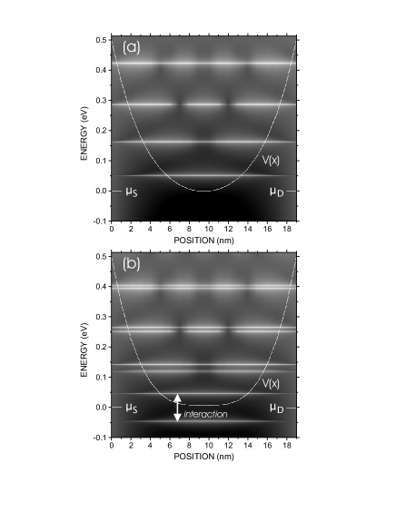
Figure 2: Spectral function $A(x,E)$ as a grayscale plot for (a) $V_{G}=0.59$V and (b) $V_{G}=0.71$V. In both cases, $V_{D}=2$mV is chosen. The resulting average electron number within the channel is (a) $N_{e}\approx 0$ and (b) $N_{e}\approx 1$ (the electron is located in the lowest resonance). The solid white line represents the mean-field potential $V(x)$, whereas $\mu_{S}$ and $\mu_{D}$ denote the chemical potentials of the source and drain contact, respectively. $T=77$K.

Fig. 2 visualizes the local density of states (LDOS) for low drain-source bias conditions and two different gate voltages $V_{G}=0.59$V and $V_{G}=0.71$V, where the average electron number in the channel becomes $N_{e}\approx 0$ and $N_{e}\approx 1$, respectively. The existence of quasi-bound states (i.e. spatially and energetically localized resonances in the spectral function $A$) yields discrete single-electron energies with associated interaction energies due to $\Sigma^{r}_{ee}$. Comparing the situation for $N_{e}=1$ with $N_{e}=0$, the single-electron resonances are moved to higher energies with respect to the lowest energy state due to the Coulomb repulsion. Note that each electron is not subject to its own Hartree potential (see lowest resonance in Fig. 2(b)) because $\Sigma^{r}_{ee}$ does not contain unphysical self-interaction energies, but includes exchange terms and correctly accounts for the electron spin. In the shown example, the next higher available state for a second electron (with opposite spin) is separated by the interaction energy $V_{00}\approx 93meV$ (see arrow in Fig. 2(b)). In general, energy levels are splitted by exchange energy terms, which have a significant influence on the energy spectrum.

As a natural consequence of $h+\Sigma^{r}_{ee}$ we therefore expect to observe the effect of a step-like electron filling (under conditions close to equilibrium in particular), energetically determined by single-electron levels and repulsion energies. This behavior in fact can be seen in Fig. 3, where the electron filling characteristics is plotted for a varying gate voltage and fixed drain-source bias $V_{D}=2$mV. Furthermore, Coulomb oscillations in the accompanying current through the channel can be identified.

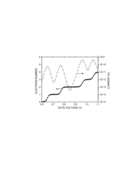
Figure 3: Single-electron tunneling characteristics for $V_{D}=2$mV. The solid line with filled squares corresponds to the average electron number within the potential well, whereas the dashed line with open circles shows the drain current, exhibiting Coulomb oscillations. $T=77$K.

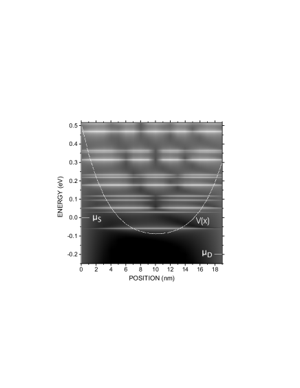
Figure 4: Nonequilibrium spectral function $A(x,E)$ as a grayscale plot for $V_{G}=0.7$V and $V_{D}=0.2$V. The resulting average electron number within the channel is $N_{e}\approx 0.22$. (The solid white line represents the mean-field potential $V(x)$, whereas $\mu_{S}$ and $\mu_{D}$ denote the chemical potentials of the source and drain contact, respectively.) $T=77$K.

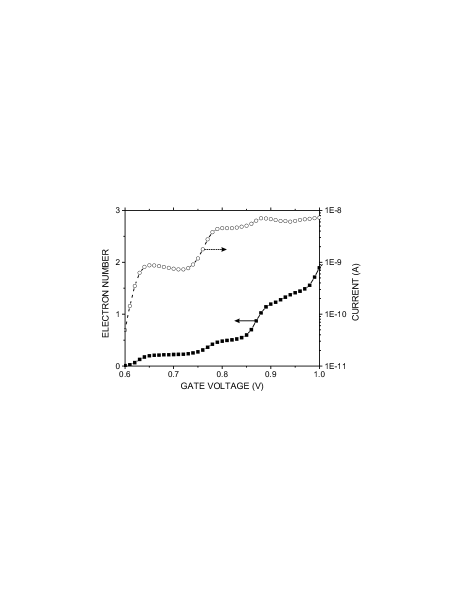
Figure 5: Transfer characteristics for $V_{D}=0.2$V. The solid line with filled squares corresponds to the average electron number within the potential well, whereas the dashed line with open circles shows the drain current through the channel. $T=77$K.

Figure 6: Output characteristics for $V_{G}=0.59$V and $V_{G}=0.71$V. $T=77$K.

Models solely based on a selfconsistent Hartree potential do not provide such quantization effects due to Coulomb repulsion. With a Hartree approach (as used with conventional Schrödinger-Poisson solvers), spectral features are solely shifted in energy, depending on the average electron density. In contrast, the MCSCG (as well as the exact diagonalization of the isolated system) provides a superposition of fading spectra of integer electron numbers with full interaction energies, however, having spectral weights that depend on the average filling condition. The local density of states under nonequilibrium conditions as shown in Fig. 4 clearly demonstrates this behavior, where the average electron number within the well is $N_{e}\approx 0.22$. In fact, the expectation value of the electron number need not be an integer, especially under non-equilibrium bias conditions, which can be seen in the corresponding transfer characteristics of the system as plotted in Fig. 5. Furthermore, Fig. 6 visualizes the output IV characteristics, where a finite drain voltage is required to pull the chemical potential of the drain contact below the lowest energy level. These results clearly demonstrate the strengths of the MCSCG approach, being able to describe single-electron charging effects under nonequilibrium bias conditions with fluctuating electron numbers.

In general, we expect the many-body Coulomb interaction to have a significant impact on the electrical behavior of nano-transistors if the single-electron charging energy becomes $\geq 4kT$, having consequences for the transconductance, onset/pinch-off voltages, sub-threshold currents, and system capacitance. A more detailed discussion of these aspects will be published elsewhere.

VII Conclusion

The Coulomb Green’s function of a one-dimensional FET in combination with a quantum kinetic description of electronic transport enables us to describe many-body charging effects within the transistor channel. We have presented a multi-configurational self-consistent Green’s function algorithm, which is able to cope with fluctuating electron numbers under nonequilibrium conditions. In the discussed example of a nano-FET with Schottky-barrier injectors, we have visualized how single-electron charging effects arise naturally as a consequence of the many-body Coulomb repulsion between quasi-bound states. The usage of a Green’s function formulation permits the systematic extension to further Coulomb diagrams and the consistent inclusion of phonon scattering.

With the presented theoretical approach, we are able to describe electronic transport and quantum charging effects in 1D nano-transistors such as gated carbon nanotubes, semiconductor whiskers, and 1D CMOS transistors (in coaxial and multi-gate planar geometry).

References

- Auth and Plummer (1997) C. P. Auth and J. D. Plummer, IEEE Electron Dev. Lett. 18, 74 (1997).
- Wong (2002) H.-S. P. Wong, IBM J. Res. & Dev. 46, 133 (2002).
- Javey et al. (2004) A. Javey, J. Guo, M. Paulsson, Q. Wang, D. Mann, M. Lundstrom, and H. Dai, Phys. Rev. Lett. 92, 106804 (2004).
- Lin et al. (2005) Y.-M. Lin, J. Appenzeller, J. Knoch, and P. Avouris, cond-mat/0501690 (2005), accepted for publication in IEEE Trans. Nanotechnol.
- McAlpine et al. (2003) M. C. McAlpine, R. S. Fiedman, S. Jin, K.-H. Lin, W. U. Wang, and C. M. Lieber, Nano Lett. 3, 1531 (2003).
- Thelander et al. (2003) C. Thelander, T. Martensson, M. T. Bjoerk, B. J. Ohlson, M. W. Larsson, L. R. Wallenberg, and L. Samuelson, Appl. Phys. Lett. 83, 2052 (2003).
- Yoneya et al. (2001) N. Yoneya, E. Watanabe, K. Tsukagoshi, and Y. Aoyagi, Appl. Phys. Lett. 79, 1465 (2001).
- Suzuki et al. (2002) M. Suzuki, K. Ishibashi, K. Toratani, D. Tsuya, and Y. Aoyagi, Appl. Phys. Lett. 81, 2273 (2002).
- Amlani et al. (2003) I. Amlani, R. Zhang, J. Tresek, and R. K. Tsui, J. Vac. Sci. Technol. B 21, 2848 (2003).
- Lake et al. (1997) R. Lake, G. Klimeck, R. C. Bowen, and D. Jovanovic, J. Appl. Phys. 81, 7845 (1997).
- Yongqiang et al. (2002) X. Yongqiang, S. Datta, and M. A. Ratner, J. Chem. Phys. 281, 151 (2002).
- Yongqiang et al. (2001) X. Yongqiang, S. Datta, and M. A. Ratner, J. Comp. Phys. 115, 4292 (2001).
- Beenakker (1991) C. W. J. Beenakker, Phys. Rev. B 44, 1646 (1991).
- Averin et al. (1991) D. V. Averin, A. N. Korotkov, and K. K. Likharev, Phys. Rev. B 44, 6199 (1991).
- Jovanovic and Leburton (1993) D. Jovanovic and J.-P. Leburton, Phys. Rev. B 49, 7474 (1993).
- Weimann et al. (1995) D. Weimann, W. Häusler, and B. Kramer, Phys. Rev. Lett. 74, 984 (1995).
- Tanaka and Akera (1996) Y. Tanaka and H. Akera, Phys. Rev. B 53, 3901 (1996).
- Pfannkuche and Ulloa (1995) D. Pfannkuche and S. E. Ulloa, Phys. Rev. Lett. 74, 1194 (1995).
- Indlekofer and Lüth (2000) K. M. Indlekofer and H. Lüth, Phys. Rev. B 62, 13016 (2000).
- Pikus and Likharev (1997) F. G. Pikus and K. K. Likharev, Appl. Phys. Lett. 71, 3661 (1997).
- Vogl et al. (1983) P. Vogl, H. P. Hjalmarson, and J. D. Dow, J. Phys. Chem. Solids 44, 365 (1983).
- Støvneng and Lipavský (1994) J. A. Støvneng and P. Lipavský, Phys. Rev. B 49, 16494 (1994).
- Schäfer and Wegener (2002) W. Schäfer and M. Wegener, Semiconductor Optics and Transport Phenomena (Springer-Verlag, 2002).
- Haug and Jauho (1998) H. Haug and A.-P. Jauho, Quantum Kinetics in Transport and Optics of Semiconductors (Springer-Verlag, 1998).
- Datta (1995) S. Datta, Electronic Transport in Mesoscopic Systems (Cambridge University Press, 1995).
- Henrickson et al. (1994) L. E. Henrickson, A. J. Glick, G. W. Bryant, and D. F. Barbe, Phys. Rev. B 50, 4482 (1994).
- Indlekofer et al. (1996) K. M. Indlekofer, J. Lange, A. Förster, and H. Lüth, Phys. Rev. B 53, 7392 (1996).
- Indlekofer et al. (2002) K. M. Indlekofer, J. P. Bird, R. Akis, D. K. Ferry, and S. M. Goodnick, Appl. Phys. Lett. 81, 2861 (2002).
- Indlekofer et al. (2003) K. M. Indlekofer, J. P. Bird, R. Akis, D. K. Ferry, and S. M. Goodnick, J. Phys.: Condens. Matter 15, 147 (2003).
- Schmidt and Gordon (1998) M. W. Schmidt and M. S. Gordon, Ann. Rev. Phys. Chem. 49, 233 (1998).