Jahn-Teller systems at half filling:
crossover from Heisenberg to Ising behavior

Abstract:

The Jahn-Teller model with $E\otimes\beta$ electron-phonon coupling and local (Hubbard-like) Coulomb interaction is considered to describe a lattice system with two orbitals per site at half filling. Starting from a state with one electron per site, we follow the tunneling of the electrons and the associated creation of an arbitrary number of phonons due to electron-phonon interaction. For this purpose we apply a recursive method which allows us to organize systematically the number of pairs of empty/doubly occupied sites and to include infinitely many phonons which are induced by electronic tunneling. In lowest order of the recursion (i.e. for all processes with only one pairs of empty/doubly occupied sites) we obtain an effective anisotropic pseudospin 1/2 Heisenberg Hamiltonian $H_{eff}$ as a description of the orbital degrees of freedom. The pseudospin coupling depends on the physical parameters and the energy. This implies that the resulting resolvent $(z-H_{eff}(z))^{-1}$ has an infinite number of poles, even for a single site. $H_{eff}$ is subject to a crossover from an isotropic Heisenberg model (weak electron-phonon coupling) to an Ising model (strong electron-phonon coupling).

1 Introduction

It has been known for a long time that orbital degrees of freedom in a systems with Jahn-Teller coupling can be described by an effective pseudospin Hamiltonian [1, 2, 3]. The coupling parameter of the pseudospin interaction is $t^{2}/U$, where $t$ is the orbital hopping rate and $U$ is the strength of the on-site Coulomb interaction. This description is of great interest because it provides a model to study orbital ordering and the possibility of orbital liquids in terms of conventional spin theories.

In this paper the influence of the electron-phonon coupling strength on the effective pseudospin Hamiltonian will studied in detail. In order to keep the calculations simple only the case of a system with $E\otimes\beta$ Jahn-Teller coupling is considered, and the electron spin is neglected. A recursive projection formalism [4] is applied to derive the effective pseudospin Hamiltonian. This approach provides pseudospin coupling parameters that depend on the electron-phonon coupling strength.

The paper is organized as follows. In Sect. 2 the model is defined. As a physical quantity the resolvent, related to the electron-phonon Hamiltonian, is considered. Its relation with physical quantities is discussed in Sect. 2.1. The recursive projection method is briefly described in Sect. 3 and the effective pseudospin Hamiltonian, obtained from this method, is presented in Sect. 4. Finally, the crossover from weak to strong electron-phonon coupling is studied in Sect. 4.1.

2 The $E\otimes\beta$ Jahn-Teller Model

The Jahn-Teller model describes fermions with pseudospin $\sigma=\uparrow,\downarrow$, coupled to phonons. It is defined by the Hamiltonian $H=H_{t}+H_{0}$, where $H_{t}$ is the hopping term of the fermions between nearest-neighbor sites ${\bf j}$ and ${\bf j}^{\prime}$

$$H_{t}=-t\sum_{<{\bf j},{\bf j}^{\prime}>}\sum_{\sigma=\uparrow,\downarrow}c_{{\bf j}\sigma}^{\dagger}c_{{\bf j}^{\prime}\sigma}+h.c.$$

and $H_{0}$ is a local (Hubbard-like) interaction and a phonon term:

$$H_{0}=\sum_{{\bf j}}\Big{[}\omega_{0}b_{\bf j}^{\dagger}b_{\bf j}+g(b_{\bf j}^{\dagger}+b_{\bf j})(n_{{\bf j}\uparrow}-n_{{\bf j}\downarrow})+Un_{{\bf j}\uparrow}n_{{\bf j}\downarrow}\Big{]}$$

for dispersionless phonons with energy $\omega_{0}$. For a given ensemble of fermions, represented by integer numbers $n_{{\bf j}\sigma}=0,1$, the Hamiltonian $H_{0}$ can be diagonalized with product states

$$\prod_{\bf j}|N_{\bf j},n_{{\bf j}\uparrow},n_{{\bf j}\downarrow}\rangle,$$

where $N_{\bf j}=0,1,...$ is the number of phonons at site ${\bf j}$. The state $|N_{\bf j},n_{{\bf j}\uparrow},n_{{\bf j}\downarrow}\rangle$ is an eigenstate of the phonon-number operator $b_{\bf j}^{\dagger}b_{\bf j}$ for $n_{{\bf j}\uparrow}=n_{{\bf j}\downarrow}=0$ and for $n_{{\bf j}\uparrow}=n_{{\bf j}\downarrow}=1$:

$$b_{\bf j}^{\dagger}b_{\bf j}|N_{{\bf j}},0,0\rangle=N_{\bf j}|N_{{\bf j}},0,0\rangle\ \ \ b_{\bf j}^{\dagger}b_{\bf j}|N_{{\bf j}},1,1\rangle=N_{\bf j}|N_{{\bf j}},1,1\rangle.$$

The corresponding eigenstates with a single fermion at ${\bf j}$ are obtained from $|N_{\bf j},0,0\rangle$ as

$$|N_{\bf j},1,0\rangle=c_{{\bf j}\uparrow}^{\dagger}\exp[-{g\over\omega_{0}}(b_{\bf j}^{\dagger}-b_{\bf j})]|N_{\bf j},0,0\rangle,\ \ \ |N_{\bf j},0,1\rangle=c_{{\bf j}\downarrow}^{\dagger}\exp[{g\over\omega_{0}}(b_{\bf j}^{\dagger}-b_{\bf j})]|N_{\bf j},0,0\rangle$$ (1)

and

$$|N_{\bf j},1,1\rangle=c_{{\bf j}\uparrow}^{\dagger}c_{{\bf j}\downarrow}^{\dagger}|N_{\bf j},0,0\rangle.$$

$\prod_{\bf j}|N_{\bf j},n_{{\bf j}\uparrow},n_{{\bf j}\downarrow}\rangle$ is an eigenstate of $H_{0}$ with energies

$$E_{0}(\{N_{\bf j},n_{{\bf j}\uparrow},n_{{\bf j}\downarrow}\})=\sum_{{\bf j}}\Big{[}\omega_{0}N_{\bf j}-{g^{2}\over\omega_{0}}(n_{{\bf j}\uparrow}-n_{{\bf j}\downarrow})^{2}+Un_{{\bf j}\uparrow}n_{{\bf j}\downarrow}\Big{]}.$$ (2)

The groundstate of $H_{0}$ has no phonons.

2.1 The Resolvent

In the following the resolvent

$$(iz+H)^{-1}$$

shall be studied. It is directly related to a number of physical quantities. One is linked with the thermodynamic properties of a statistical ensemble governed by the Hamiltonian $H$ through the Boltzmann weight at inverse temperature $\beta$. It reads

$$e^{-\beta H}=\int_{\Gamma}(iz+H)^{-1}e^{i\beta z}{dz\over 2\pi}.$$ (3)

$\Gamma$ is a closed contour that encloses all eigenvalues of $H$. Another connection is with the dynamics of quantum states in a system characterized by the Hamiltonian $H$: The evolution of a state $|\Psi_{0}\rangle$ at time 0 to a later time $t$ is given by

$$|\Psi_{t}\rangle=e^{iHt}|\Psi_{0}\rangle.$$

A Laplace transformation for positive time gives with $Imz<0$ the resolvent that acts on the initial state:

$$\int_{0}^{\infty}e^{-izt}|\Psi_{t}\rangle dt=\int_{0}^{\infty}e^{-izt}e^{iHt}dt|\Psi_{0}\rangle=(z-H)^{-1}|\Psi_{0}\rangle.$$ (4)

The return probability to the initial state is obtained from the inverse Laplace transform and reads

$$\langle\Psi_{0}|\Psi_{t}\rangle={1\over 2\pi}\int_{-\infty}^{\infty}e^{izt}\langle\Psi_{0}|(z-H)^{-1}|\Psi_{0}\rangle dz.$$ (5)

Using the spectral representation of $H$ with eigenvalues $E_{j}$, the expectation value in the integrand reads

$$\langle\Psi_{0}|(z-H)^{-1}|\Psi_{0}\rangle=\sum_{j}{|\langle E_{j}|\Psi_{0}\rangle|^{2}\over z-E_{j}}.$$

Inserting this into Eq. (5) allows us to apply Cauchy’s Theorem to perform the integration.

In order to evaluate the resolvent a standard procedure is to expanded it in terms of $H_{t}$ in a Neumann series

$$(z-H)^{-1}=(z-H_{0}-H_{t})^{-1}=(z-H_{0})^{-1}\sum_{l\geq 0}[H_{t}(z-H_{0})^{-1}]^{l}$$

and to truncate this series. The poles of any finite truncation are the eigenvalues of the unperturbed Hamiltonian $H_{0}$. This may be insufficient for a good approximation of $(z-H)^{-1}$. In the next section a recursive approach is applied that avoids this restriction.

3 Projection Formalism and Continued-Fraction Representation

Considering a half-filled system, the projected resolvent $P_{0}(z-H)^{-1}P_{0}$ must be evaluated. It is assumed that $P_{0}$ projects the states of the entire Hilbert ${\cal H}$ space to the subspace ${\cal H}_{0}$. The projected resolvent satisfies the identity

$$P_{0}(z-H)^{-1}P_{0}=\Big{[}P_{0}(z-H)P_{0}-P_{0}HP_{1}(z-H)_{1}^{-1}P_{1}HP_{0}\Big{]}_{0}^{-1},$$ (6)

where $P_{1}={\bf 1}-P_{0}$ projects onto the Hilbert space ${\cal H}_{1}$ that is complementary to ${\cal H}_{0}$. If $H$ obeys the relations

$$P_{0}HP_{1}=P_{0}HP_{2},\ \ P_{1}HP_{0}=P_{2}HP_{0}\ \ \ (P_{2}\neq P_{1}),$$

Eq. (6) can also be written as

$$P_{0}(z-H)^{-1}P_{0}=\Big{[}P_{0}(z-H)P_{0}-P_{0}HP_{2}(z-H)_{1}^{-1}P_{2}HP_{0}\Big{]}_{0}^{-1}.$$ (7)

The identity used in Eq. (6) can be applied again to $P_{2}(z-H)_{1}^{-1}P_{2}$ on the right-hand side. This procedure can be applied iteratively. It creates a hierarchy of projectors $P_{k}$ onto Hilbert spaces ${\cal H}_{k}$. It is based on the fact that the projector $P_{2j+1}$ is created from $P_{2j-1}$ and $P_{2j}$ as

$${\cal H}_{2j+1}={\cal H}_{2j-1}\backslash{\cal H}_{2j}\subset{\cal H}_{2j-1},$$

and $P_{2j+2}$ comes from the relation

$$P_{2j+1}HP_{2j}=P_{2j+2}HP_{2j}\equiv H_{j+1,j}\ \ \ {\rm and}\ \ \ P_{2j}HP_{2j+1}=P_{2j}HP_{2j+2}\equiv H_{j,j+1}.$$ (8)

In terms of the projected resolvents this construction implies a recursion relation. Using $G_{2j}=P_{2j}(z-H)_{2j-1}^{-1}P_{2j}$ and $H_{j,j+1}=P_{2j}HP_{2j+2}$ this reads

$$G_{2j}=\Big{[}z-P_{2j}HP_{2j}-H_{j,j+1}G_{2j+2}H_{j+1,j}\Big{]}_{2j}^{-1}.$$ (9)

It is useful that the Hamiltonian $H$ in Sect. 2 is the sum of two Hamiltonians $H=H_{0}+H_{1}$ and that one can choose projections such that the following holds:

(1) $H_{0}$ stays inside the projected Hilbert space: $H_{0}P_{0}=P_{0}H_{0}P_{0}$ and $P_{0}H_{0}=P_{0}H_{0}P_{0}$.

(2) $H_{1}$ maps from ${\cal H}_{2j}$ to ${\cal H}_{2j+2}$:

$$H_{1}:{\cal H}_{2j}\to{\cal H}_{2j+2},$$

where ${\cal H}_{2j}$ is orthogonal to ${\cal H}_{2j+2}$. In the next section these properties will be used to construct an effective Hamiltonian.

4 The Effective Hamiltonian

The projection formalism is now applied to the Hamiltonian $H=H_{0}+H_{t}$ of Sect. 2. The Hilbert space separates into subspaces with a fixed number of fermions with pseudospin $\uparrow$ and a fixed number with pseudospin $\downarrow$ because $H$ cannot change it with a diagonal pseudospin term. The case is considered here where $P_{0}$ projects onto singly occupied sites with no phonons. $H_{t}$ is off-diagonal with respect to the phonons and changes the number of pairs of empty/doubly-occupied sites (PEDS) by one. Therefore, $P_{2j}$ ($j\geq 1$) projects onto states with $j$ PEDS and any number of phonons. According to this construction, the matrix elements of $P_{2j}HP_{2j+2}=P_{2j}H_{t}P_{2j+2}$ and $P_{2j+2}HP_{2j}=P_{2j+2}H_{t}P_{2j}$ are all non-zero with respect to different phonon numbers. $P_{2j}H_{0}P_{2j}$ is diagonal in the basis (1) with matrix elements:

$$\omega_{0}\sum_{{\bf j}}N_{\bf j}-2(M-j)g^{2}/\omega_{0}+Uj,$$

where $2(M-j)$ counts the number of singly-occupied sites and $j$ the number of doubly-occupied sites on a lattice with $2M$ sites. Thus the recursion relation of Eq. (7) becomes

$$G_{2j}=\Big{[}z-\omega_{0}\sum_{{\bf j}}N_{\bf j}+2(M-j)2g^{2}/\omega_{0}-Uj-H_{j,j+1}G_{2j+2}H_{j,j+1}^{T}\Big{]}_{2j}^{-1}$$ (10)

with $H_{j,j+1}$ defined in Eq. (8). The recursion terminates on a finite lattice ($M<\infty$) if $j=M$, since at most $M$ PEDS can be created and, therefore, $P_{2M+1}$ is a projection onto the empty space. $G_{2M}$ is diagonal with matrix elements

$${1\over z-\omega_{0}\sum_{{\bf j}}N_{\bf j}-UM}.$$

This can serve as a starting point for the iterative approximation of $G_{0}$. On the other hand, we can express $G_{0}$ by $G_{2}$ through Eq. (10) and approximate $G_{2}$ by the diagonal matrix

$$G_{2}\approx[z-\omega_{0}\sum_{{\bf j}}b^{\dagger}_{\bf j}b_{\bf j}+2(M-1)g^{2}/\omega_{0}-U]_{2}^{-1}.$$ (11)

This approximation corresponds with a truncation of all scattering processes with more than one PEDS. It is valid for weak hopping, i.e. for $t/\omega_{0}$ small in comparison with $g/\omega_{0}$ and $U/\omega_{0}$. Subsequently, it will turn out that an effective expansion parameter for the truncation is $t^{2}/(U/\omega_{0}+2g^{2}/\omega_{0}^{2})$.

Eq. (11) gives for $G_{0}$ the expression

$$G_{0}=\Big{[}z+2Mg^{2}/\omega_{0}-H_{0,1}[z-\omega_{0}\sum_{{\bf j}}b^{\dagger}_{\bf j}b_{\bf j}+2(M-1)g^{2}/\omega_{0}-U]_{2}^{-1}H_{0,1}^{T}\Big{]}_{0}^{-1}.$$ (12)

$H_{0,1}[...]_{2}^{-1}H_{0,1}^{T}$ is a matrix in a Hilbert space without phonons according to the definition of $P_{0}$. $H_{0,1}^{T}$ creates phonons as well as a PEDS. This will be picked up by the diagonal matrix $[...]_{2}^{-1}$. Finally, $H_{0,1}$ annihilates the phonons and the PEDS. Consequently, the entire expression is either diagonal or has off-diagonal elements with nearest-neigbor pseudospin exchanges. Such a matrix can be expressed by a (anisotropic) pseudospin-1/2 Hamiltonian. A detailed calculation gives an anisotropic Heisenberg Hamiltonian

$$H_{eff}\equiv-2Mg^{2}/\omega_{0}+H_{0,1}[z-\omega_{0}\sum_{{\bf j}}b^{\dagger}_{\bf j}b_{\bf j}+2(M-1)g^{2}/\omega_{0}-U]_{2}^{-1}H_{0,1}^{T}$$

$$=-2Mg^{2}/\omega_{0}+\sum_{{\bf j},{\bf j}^{\prime}}\Big{[}a_{\uparrow\uparrow}(S_{\bf j}^{z}S_{{\bf j}^{\prime}}^{z}-{1\over 4})+a_{\uparrow\downarrow}(S_{\bf j}^{x}S_{{\bf j}^{\prime}}^{x}+S_{\bf j}^{y}S_{{\bf j}^{\prime}}^{y})\Big{]}$$ (13)

with the pseudospin-1/2 operators $S^{x},S^{y},S^{z}$ and $z$-dependent coupling coefficients (cf. Appendix A)

$$a_{\uparrow\uparrow}=2t^{2}{e^{-2g^{2}/\omega_{0}^{2}}\over\omega_{0}}\gamma^{*}({U-z-2(M-1)g^{2}/\omega_{0}\over\omega_{0}},-2g^{2}/\omega_{0}^{2})$$

$$a_{\uparrow\downarrow}=2t^{2}{e^{-2g^{2}/\omega_{0}^{2}}\over\omega_{0}}\gamma^{*}({U-z-2(M-1)g^{2}/\omega_{0})\over\omega_{0}},2g^{2}/\omega_{0}^{2}).$$

$\gamma^{*}$ is the incomplete Gamma function [7]:

$$\gamma^{*}(a,y)=\sum_{m\geq 0}{1\over m!}{(-y)^{m}\over a+m}.$$

Introducing the system energy $E=z+2Mg^{2}/\omega_{0}$ we can write $(z-H_{eff})^{-1}=(E-H_{H})^{-1},$ where $H_{H}$ is the Heisenberg Hamiltonian:

$$H_{H}=\sum_{{\bf j},{\bf j}^{\prime}}\Big{[}a_{\uparrow\uparrow}(S_{\bf j}^{z}S_{{\bf j}^{\prime}}^{z}-{1\over 4})+a_{\uparrow\downarrow}(S_{\bf j}^{x}S_{{\bf j}^{\prime}}^{x}+S_{\bf j}^{y}S_{{\bf j}^{\prime}}^{y})\Big{]}.$$ (14)

Now the coupling coefficients depend on the number of lattice sites $M$ only through $E$:

$$a_{\uparrow\uparrow}=2t^{2}{e^{-2g^{2}/\omega_{0}^{2}}\over\omega_{0}}\gamma^{*}({U+2g^{2}/\omega_{0}-E\over\omega_{0}},-2g^{2}/\omega_{0}^{2})$$

$$a_{\uparrow\downarrow}=2t^{2}{e^{-2g^{2}/\omega_{0}^{2}}\over\omega_{0}}\gamma^{*}({U+2g^{2}/\omega_{0})-E\over\omega_{0}},2g^{2}/\omega_{0}^{2}).$$ (15)

4.1 Crossover from Weak to Strong Electron-Phonon Coupling

The energy-dependent coefficients in $H_{eff}$ simplify substantially for weak and strong coupling. Relevant are low energies $E$ which represent the poles of the resolvent in Eq. (3). To avoid the poles of the incomplete Gamma function, the following discussion is restricted to energies

$$E\leq U+2g^{2}/\omega_{0}.$$ (16)

It will be shown that in this case there exist poles of the projected Green’s function with $E_{j}\leq 0$. The restriction (16) implies that the approximated diagonal Green’s function $G_{2}$ in Eq. (11) has only negative matrix elements:

$$G_{2}=(E-2g^{2}/\omega_{0}-U-\sum_{\bf j}N_{\bf j})_{2}^{-1}<0.$$

Thus $H_{0,1}G_{2}H_{0,1}^{T}$ is a negative matrix and the projected Green’s function

$$(E-H_{0,1}G_{2}H_{0,1}^{T})_{0}^{-1}$$

has all poles $E_{j}$ on the negative real axis. The relevant parameter in our truncated continued fraction is $U/\omega_{0}+2g^{2}/\omega_{0}^{2}\gg 1$. This allows a free tuning of the electron-phonon coupling $g$, as long as $U$ is sufficiently large.

The weak-coupling limit corresponds with the Hubbard model. For the latter (i.e. for $g=0$) it is known that a $1/U$ expansion at half filling gives in leading order an isotropic Heisenberg model with coupling coefficients [5]

$$a_{\uparrow\uparrow}=a_{\uparrow\downarrow}={2t^{2}\over U}.$$

A similar result was obtained for the Holstein model [6]. It should be noticed that the energy dependence disappears in this expansion. For nonzero but small $g$ ($g/\omega_{0}\ll 1$) the coupling coefficients of Eq. (15) have the asymptotic behavior

$$a_{\uparrow\uparrow}\sim a_{\uparrow\downarrow}\sim{2t^{2}\over 2g^{2}/\omega_{0}+U-E}.$$

In the opposite regime, where the electron-phonon coupling is strong (i.e. $g/\omega_{0}\gg 1$), the incomplete Gamma function is approximated by

$$\gamma^{*}({U+2g^{2}/\omega_{0}-E\over\omega_{0}},\mp 2g^{2}/\omega_{0}^{2})\sim{\omega_{0}\over U+2g^{2}/\omega_{0}-E}\sum_{m\geq 0}{1\over m!}(\pm 2g^{2}/\omega_{0}^{2})^{m}={\omega_{0}e^{\pm 2g^{2}/\omega_{0}^{2}}\over U+2g^{2}/\omega_{0}-E}.$$

Thus the coupling coefficients of the pseudospin-1/2 Hamiltonian are

$$a_{\uparrow\uparrow}\sim{2t^{2}\over 2g^{2}/\omega_{0}+U-E},\ \ \ \ a_{\uparrow\downarrow}\sim 0.$$

In this limit the effective Hamiltonian is diagonal and accidentally degenerate.

The crossover regime, within the restriction of Eq. (16), is shown in Fig. 1. It indicates that at weak electron-phonon coupling there is a strong isotropic pseudospin-pseudospin coupling, whereas a strong electron-phonon coupling implies a strong pseudospin-pseudospin coupling only for the $S^{z}$ component but a weak one for $S^{x}$ and $S^{y}$. Thus the tuning of the electron-phonon interaction is given by a crossover from an isotropic Heisenberg to an Ising model. This may be accompanied by a sequence of crossovers and/or phase transitions.

The pole from the groundstate of the projected resolvent $(E-H_{H})^{-1}$ is easily evaluated in the asymptotic regimes. For the weak-coupling regime it is

$$E_{H}=g^{2}/\omega_{0}+U/2-\sqrt{(g^{2}/\omega_{0}+U/2)^{2}-2t^{2}\lambda_{H}}$$

and for the strong-coupling regime

$$E_{I}=g^{2}/\omega_{0}+U/2-\sqrt{(g^{2}/\omega_{0}+U/2)^{2}-2t^{2}\lambda_{I}},$$

where $\lambda_{H}$ ($\lambda_{I}$) is the lowest eigenvalue of the isotropic Heisenberg (Ising) Hamiltonian with unit coupling, respectively.

5 Conclusions

Starting from a Hamiltonian with short-range Coulomb and $E\otimes\beta$ Jahn-Teller interaction, a system of spinless fermions was studied at half filling. An effective Hamiltonian $H_{eff}$ was derived under the assumption that the kinetic energy (i.e. the hopping term) is always dominated by the local interaction energy. In the absence of the electron-phonon interaction this leads to the well-known isotropic pseudospin-1/2 Heisenberg Hamiltonian for $H_{eff}$. A weak electron-phonon interaction suppresses the pseudospin-1/2 interaction of the effective Hamiltonian, and an increasing electron-phonon interaction develops an anisotropy, where the pseudospin-pseudospin interaction in the $xy$ plane decreases like $\exp(-4g^{2}/\omega_{0}^{2})$ with the electron-phonon coupling constant $g$ and the pseudospin-pseudospin interaction in the $z$ direction decreases like $1/g^{2}$.

Acknowledgement:

The author is grateful to K.-H. Höck, P. Riseborough, and D. Schneider for interesting discussions. This work was supported by the Deutsche Forschungsgemeinschaft through Sonderforschungsbereich 484.

Appendix A

$$a_{\uparrow\uparrow}:=2t^{2}\sum_{m,m^{\prime}\geq 0}{\langle 0,\uparrow|m,0,0\rangle\langle m,0,0|0,\uparrow\rangle\langle 0,\downarrow|m^{\prime},0,0\rangle\langle m^{\prime},0,0|0,\downarrow\rangle\over z-[\omega_{0}(m+m^{\prime})-(N-2)g^{2}/\omega_{0}+U]}$$

$$=2t^{2}e^{-2g^{2}/\omega_{0}^{2}}\sum_{m,m^{\prime}\geq 0}{1\over m!m^{\prime}!}{(g^{2}/\omega_{0})^{m+m^{\prime}}\over z-[\omega_{0}(m+m^{\prime})-(N-2)g^{2}/\omega_{0}+U]}.$$

The double sum is reduced to a single sum

$$=2t^{2}e^{-2g^{2}/\omega_{0}^{2}}\sum_{m\geq 0}{1\over m!}{(2g^{2}/\omega_{0})^{m}\over z-\omega_{0}m+(N-2)g^{2}/\omega_{0}-U}$$

and

$$a_{\uparrow\downarrow}:=2t^{2}\sum_{m,m^{\prime}\geq 0}{\langle 0,\uparrow|m,0,0\rangle\langle m,0,0|0,\downarrow\rangle\langle 0,\downarrow|m^{\prime},0,0\rangle\langle m^{\prime},0,0|0,\uparrow\rangle\over z-[\omega_{0}(m+m^{\prime})-(N-2)g^{2}/\omega_{0}+U]}$$

$$=2t^{2}e^{-2g^{2}/\omega_{0}^{2}}\sum_{m,m^{\prime}\geq 0}{1\over m!m^{\prime}!}{(-g^{2}/\omega_{0})^{m+m^{\prime}}\over z-[\omega_{0}(m+m^{\prime})-(N-2)g^{2}/\omega_{0}+U]}$$

The double sum is again reduced to a single sum

$$=2t^{2}e^{-2g^{2}/\omega_{0}^{2}}\sum_{m\geq 0}{1\over m!}{(-2g^{2}/\omega_{0})^{m}\over z-\omega_{0}m+(N-2)g^{2}/\omega_{0}-U}.$$

These expressions are related to the incomplete Gamma function [7]

$$\gamma^{*}(a,y)=\sum_{m\geq 0}{1\over m!}{(-y)^{m}\over a+m}$$

such that

$$a_{\uparrow\uparrow}=2t^{2}{e^{-2g^{2}/\omega_{0}^{2}}\over\omega_{0}}\gamma^{*}({U-z-2(M-1)g^{2}/\omega_{0}\over\omega_{0}},-2g^{2}/\omega_{0}^{2})$$

$$a_{\uparrow\downarrow}=2t^{2}{e^{-2g^{2}/\omega_{0}^{2}}\over\omega_{0}}\gamma^{*}({U-z-2(M-1)g^{2}/\omega_{0})\over\omega_{0}},2g^{2}/\omega_{0}^{2}).$$

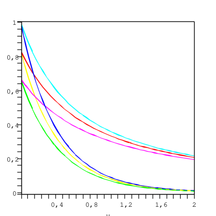
Figure 1: Coupling coefficients of the effective pseudospin-1/2 Hamiltonian of Eq. (14) as a function of $y=2g^{2}/\omega_{0}^{2}$: $a_{\uparrow\uparrow}$ (upper set of curves) and $a_{\uparrow\downarrow}$ (lower set of curves) in units of $t^{2}/\omega_{0}$ for $(U-E)/\omega_{0}=1.0,1.2,1.5$ (from top to bottom in each set of curves).

References

• [1] K.I. Kugel and D.I. Khomskii, Sov. Phys. - JETP 37, 725 (1973)
• [2] L.F. Feiner, A.M. OleΕ›, and J. Zaanen, Phys. Rev. Lett. 78, 2799 (1997)
• [3] A.B. Harris et al., Phys. Rev. B 69, 094409 (2004)
• [4] K. Ziegler, Phys. Rev. A 68, 053602 (2003)
• [5] P. Fulde, Electron Correlations in Molecules and Solids, Springer (Berlin 1993)
• [6] J.K. Freericks, Phys. Rev. B 48, 3881 (1993)
• [7] M. Abramowitz and I.A. Stegun, Handbook of Mathematical Functions, Dover, (New York 1965)