Temperature in One-Dimensional Bosonic Mott Insulators

Abstract

The Mott insulating phase of a one-dimensional bosonic gas trapped in optical lattices is described by a Bose-Hubbard model. A continuous unitary transformation is used to map this model onto an effective model conserving the number of elementary excitations. We obtain quantitative results for the kinetics and for the spectral weights of the low-energy excitations for a broad range of parameters in the insulating phase. By these results, recent Bragg spectroscopy experiments are explained. Evidence for a significant temperature of the order of the microscopic energy scales is found.

I Introduction

Ultracold atoms in optical lattices provide tunable experimental realizations of correlated many-particle systems. Even the dimensionality of these systems can be chosen between one and three. Recently, the transition between superfluid and Mott insulating (MI) phases has been observed by tuning the ratio between the kinetic and the interaction energy Greiner et al. (2002); Paredes et al. (2004). Dynamical aspects can also be addressed experimentally Stöferle et al. (2004); Köhl et al. (2005).

There are many theoretical treatments of these issues, ranging from mean-field approaches Jaksch et al. (1998) to more sophisticated techniques Fisher et al. (1989); Pai et al. (1996); Kashurnikov and Svistunov (1996); Kühner and Monien (1998); Elstner and Monien (1999); Kühner et al. (2000). The transition at zero temperature ($T=0$) has been analyzed in one-dimensional systems Pai et al. (1996); Kashurnikov and Svistunov (1996); Kühner and Monien (1998); Elstner and Monien (1999); Kühner et al. (2000). But there is still a multitude of open questions. Our aim is to explain the dynamics of the excitations which has moved in the focus recently Stöferle et al. (2004); Köhl et al. (2005); Batrouni et al. (2005).

The present work is intended to clarify the significance of various excitation processes depending on the kinetic and the interaction energy and on the temperature. To this end, we will analyze the spectral weights of the one-dimensional MI phase with one boson per site $n=1$.

The low-energy excitations are either double occupancies ($n=2$), which we will call ‘particles’, or they are holes ($n=0$). Both excitations are gapped as long as the system is insulating. They become soft at the quantum critical point which separates the insulator from the superfluid. We use a continuous unitary transformation (CUT) Wegner (1994); Knetter and Uhrig (2000) to obtain an effective Hamiltonian in terms of the elementary excitations ‘particle’ and ‘hole’. This effective Hamiltonian conserves the number of particles and of holes Knetter et al. (2003). The CUT is realized in real space in close analogy to the derivation of the generalized $t$-$J$ model from the Hubbard model Reischl et al. (2004). The strongly correlated many-boson problem is reduced to a problem involving a small number of particles and holes. This simplification enables us to calculate kinetic properties like the dispersions and spectral properties like spectral weights.

The article is set-up as follows. First, the model and the relevant observable are introduced (Sect. II). Then, the method used is presented and described (Sect. III). The spectral weights are computed in Sect. IV. In Sect. V, the experiment is analyzed which requires calculations at finite temperatures as well. Finally, the results are discussed in Sect. VI.

II Model

To be specific, we study the Bose-Hubbard model $H=tH_{t}+UH_{U}$ in one dimension

$$H=-t\sum\limits_{i}(b^{\dagger}_{i}b^{\phantom{\dagger}}_{i+1}+b^{\dagger}_{i+1}b^{\phantom{\dagger}}_{i})+(U/2)\sum_{i}\hat{n}_{i}(\hat{n}_{i}-1)$$ (1)

where the first term is the kinetic part $tH_{t}$ and the second term the repulsive interaction $UH_{U}$ with $U>0$. The bosonic annihilation (creation) operators are denoted by $b^{(\dagger)}_{i}$, the number of bosons by $\hat{n}_{i}=b^{\dagger}_{i}b^{\phantom{\dagger}}_{i}$. If needed the term $H_{\mu}=-\mu\sum_{i}\hat{n}_{i}$ is added to $H$ to control the particle number. For numerical simplicity, we truncate the local bosonic Hilbert space to four states. This does not change the relevant physics significantly Pai et al. (1996); Kashurnikov and Svistunov (1996); Kühner and Monien (1998).

Besides the Hamiltonian we need to specify the excitation operator $R$. In the set-up of Refs. Stöferle et al., 2004 and Köhl et al., 2005 the depth of the optical lattices is changed periodically to excite the system. In terms of the tight binding model (1) this amounts to a periodic change of $t$ and of $U$ leading to

$$R\propto\delta tH_{t}+\delta UH_{U}\ .$$ (2)

Since multiples of $H$ do not induce excitations we consider

$$R\to\tilde{R}=R-(\delta U/U)H\ .$$ (3)

Both operators $R$ and $\tilde{R}$ induce the same transitions $\langle n|R|m\rangle=\langle n|\tilde{R}|m\rangle$ where $|n\rangle\neq|m\rangle$ are eigen states of $H$. Eventually, the relevant part of $R$ is proportional to $H_{t}$. For simplicity, we set the factor of proportionality to one.

If the interaction dominates ($U/t\to\infty$) the ground state of (1) is the product state of precisely one boson per site $|\text{ref}\rangle=|1\rangle_{1}\otimes|1\rangle_{2}\ldots\otimes|1\rangle_{N}$, where $|n\rangle_{i}$ denotes the local state at site $i$ with $n$ bosons. We take $|\text{ref}\rangle$ as our reference state; all deviations from $|\text{ref}\rangle$ are considered as elementary excitations. Since we restrict our calculation to four states per site we define three creation operators: $h^{\dagger}_{i}|1\rangle_{i}=|0\rangle_{i}$ induces a hole at site $i$, $p^{\dagger}_{i}|1\rangle_{i}=|2\rangle_{i}$ induces a particle at site $i$, and $d^{\dagger}_{i}|1\rangle_{i}=|3\rangle_{i}$ induces a double-particle at site $i$. The operators $h$, $p$ and $d$ obey the commutation relations for hardcore bosons.

III CUT

The Hamiltonian (1) conserves the number of bosons $b$. But if it is rewritten in terms of $h,p$, and $d$ it is no longer particle-conserving, e.g., the application of $H_{t}$ to $|\text{ref}\rangle$ generates a particle-hole pair. We use a CUT defined by

$$\partial_{l}H(l)=[\eta(l),H(l)]$$ (4)

to transform $H(l=0)=H$ from its form in (1) to an effective Hamiltonian $H_{\text{eff}}:=H(l=\infty)$ which conserves the number of elementary excitations, i.e., $[H_{U},H_{\text{eff}}]=0$. An appropriate choice of the infinitesimal generator $\eta$ is defined by the matrix elements

$$\eta_{i,j}(l)={\rm sgn}\left(q_{i}-q_{j}\right)H_{i,j}(l)$$ (5)

in an eigen basis of $H_{U}$; $q_{i}$ is the corresponding eigenvalue Knetter and Uhrig (2000). The structure of the resulting $H_{\text{eff}}$ and the implementation of the flow equation in second quantization in real space is described in detail in Refs. Knetter et al., 2003 and Reischl et al., 2004.

Figure 1: Residual off-diagonality for values of $t/U\in\{0.1,0.2\}$ for maximal $r=2$ and $r=3$. Inset: Magnification for small values of the flow parameter $l$. The ROD for $r=3$ and $t/U=0.2$ displays non-monotonic behavior. In this case, we stop the flow at the first minimum of the ROD. Its position is indicated by a vertical line.

The flow equation (4) generates a proliferating number of terms. For increasing $l$, more and more hardcore bosons are involved, e.g., annihilation and creation of three bosons $p^{\dagger}_{i}p^{\dagger}_{i+1}p^{\dagger}_{i+2}p^{\phantom{\dagger}}_{i}p^{\phantom{\dagger}}_{i+1}p^{\phantom{\dagger}}_{i+2}$, and processes over a larger and larger range occur, e.g., hopping over $j$ sites $p^{\dagger}_{i+j}p^{\phantom{\dagger}}_{i}$. To keep the number of terms finite we omit normal-ordered terms beyond a certain extension $r$. Normal-ordering means that the creation operators of the elementary excitations appear to the left of the annihilation operators. If terms appear which are not normal-ordered the commutation relations are applied to rewrite them in normal-ordered form. The normal-ordering is important since it ensures that only less important terms are omitted. Generically, such terms involve more particles Knetter et al. (2003); Reischl et al. (2004).

We define the extension $r$ as the distance between the rightmost and the leftmost creation or annihilation operator in a term Knetter et al. (2003); Reischl et al. (2004). The extension $r$ of a term measures the range of the physical process which is described by this term. So our restriction to a finite extension restricts the range of processes kept in the description. This is the most serious restriction in our approach. Note that the extension $r$ implies for hardcore bosons that at maximum $r+1$ bosons are involved.

For $l<\infty$, $H(l)$ still contains terms like $p^{\dagger}_{i}h^{\dagger}_{i+1}$ which do not conserve the number of particles. To measure the extent to which $H(l)$ deviates from the desired particle-conserving form, we introduce the residual off-diagonality (ROD) as the sum of the moduli squared of the coefficients of all terms which change the number of elementary excitations. The ROD for maximal extensions $r=2$ and $r=3$ is shown in Fig. 1. Ideally, the ROD decreases monotonically with $l$. The calculation with $r=2$ indeed shows the desired monotonic behavior of the ROD for all values of $t/U$.

But non-monotonic behavior can also occur Reischl et al. (2004). It is observed in Fig. 1 for extension $r=3$. While for small $t/U$ the ROD still decays monotonically it displays non-monotonic behavior for larger $t/U$, see e.g. the ROD for $t/U=0.2$ and $r=3$ in Fig. 1. An uprise at larger values $l\gtrapprox 1/t$ signals that the intended transformation cannot be performed in a well-controlled way. The uprise stems from matrix elements which do not decrease but increase, at least in an intermediate interval of the running variable $l$. Such an increase occurs if the number of excitations is not correlated with the total energy of the states. This means that two states are linked by an off-diagonal matrix element of which the state with low number of excitations is higher in total energy than the state with a higher number of excitations. The increase of such a matrix element bears the risk that the unavoidable truncations imply a too severe approximation.

The situation that the number of excitations is not correlated with the total energy can occur where the lower band edge of a continuum of more particles falls below the upper band edge of a continuum of less particles or below the dispersion of a single excitation, see, e.g., Ref. Schmidt and Uhrig, 2005. This situation implies additional life-time effects since the states with less particles can decay into the states with more particles. Even if the decay rates are very small the CUT can be spoilt by them because the CUT in its form defined by Eq. (5) correlates the particle number and the energy of the states.

In order to proceed in a controlled way, we neglect the small life-time effects if they occur at all. This is done by stopping the CUT at $l_{\text{min}}$ at the first minimum of the ROD. The position of $l_{\text{min}}$ for $t/U=0.2$ and $r=3$ is indicated in the inset of Fig. 1 by a vertical line. It is found that the remaining values of the ROD are small and thus negligible. Hence we omit the remaining off-diagonal terms. Only close to the critical point, where the MI phase vanishes, the present approach becomes insufficient.

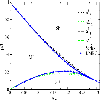
Figure 2: (color online) Phase diagram of the Mott insulating (MI) and the superfluid (SF) phase in the $(t/U,\mu/U)$ plane. Dotted (dashed) lines show CUT results for maximal extension $r=2$ ($r=3$). Solid lines (symbols) show series (DMRG) results from Refs. Elstner and Monien, 1999 and Kühner and Monien, 1998.

We check the reliability of our approach by comparing its results to those of other methods for the phase diagram in Fig. 2. The upper boundary of the MI phase is given by the particle gap $\Delta^{\text{p}}:=\text{min}_{k}\omega^{\text{p}}(k)$. The lower boundary is given by the negative hole gap $-\Delta^{\text{h}}$ where $\Delta^{\text{h}}:=\text{min}_{k}\omega^{\text{h}}(k)$. The dotted (dashed) curves result from CUTs for $r=2$ ($r=3$). For $r=2$, the CUT can be performed till $l=\infty$; for $r=3$, the flow is stopped at $l_{\text{min}}$. Solid curves depict the findings by series expansion, the symbols those obtained by DMRG Elstner and Monien (1999); Kühner and Monien (1998). The agreement is very good in view of the truncation of the Hilbert space and in view of the low value of $r$. Note that the $r=3$ result agrees better with the series and DMRG results than the $r=2$ result. As expected, the deviations increase for larger values of $t$ because longer-range processes become more important. Yet the values obtained by the CUT for the critical ratio $x_{c}:=t/U$, where the MI phase vanishes, are reasonable. We find $x_{c}^{(r=2)}=0.271$ and $x_{c}^{(r=3)}=0.258$. By high accuracy density-matrix renormalization $x_{c}=0.297\pm 0.01$ was found, see Ref. Kühner et al., 2000 and references therein. Series expansion provides $x_{c}=0.26\pm 0.01$ which is very close to our value $x_{c}^{(r=3)}$. This fact underlines the similarity between series expansions and the real space CUT as employed in the present work.

We conclude from the above findings for the phase diagram (Fig. 2) that the mapping to the particle-conserving $H_{\text{eff}}$ works very well for large parts of the phase diagram. It does not, however, capture the Kosterlitz-Thouless nature of the transition itself Kühner et al. (2000). The CUT yields reliable results within the MI phase for $t\lessapprox 0.2U$. Henceforth, results for this regime will be shown which were obtained in the $r=3$ scheme.

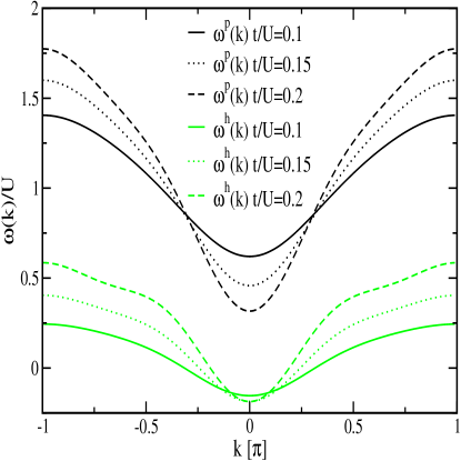
Figure 3: (color online) The dispersions of a particle $\omega^{\rm p}(k)$ (black) and a hole $\omega^{\rm h}(k)$ (green/grey) for $t=0.1U$ (solid), $t=0.15U$ (dotted) and $t=0.2U$ (dashed).

In Fig. 3, the single-particle dispersion $\omega^{\rm p}(k)$ (one-hole dispersion $\omega^{\rm h}(k)$) is shown as black (green or grey, resp.) curves. Both dispersions increase with $t$; the particle dispersion always exceeds the hole dispersion. On increasing $t$, the center of the hole dispersion shifts to higher energies while the center of the particle dispersion remains fairly constant in energy.

IV Observable

At the beginning of the flow ($l=0$), the observable $R$ is proportional to $H_{t}$. The dynamic structure factor $S_{R}(k,\omega)$ encodes the response of the system to the application of the observable $R$. The observable $R$ transfers no momentum because it is invariant with respect to translations. Therefore, the Bragg spectroscopy Stöferle et al. (2004); Köhl et al. (2005) measures the response $S_{R}(k=0,\omega)$ at momentum $k=0$ and energy $\omega$. A sketch of the spectral density $S_{R}(k=0,\omega)$ for this observable is shown in Fig. 4. We assume that the average energy is mainly determined by $H_{U}$ in the MI regime. Then the first continuum is located at $U$ and a second one at $2U$. For small $t/U$ the continua will be well separated. The energy-integrated spectral density in the first continuum is the spectral weight $S_{1}$. Correspondingly, $S_{2}$ stands for the spectral weight in the second continuum.

To analyze the spectral weights in the effective model obtained by the CUT the observable $R$ must be transformed as well. Before the CUT, the observable is $R(l=0)=H_{t}$. It is a sum of local terms

$$R(l=0)=H_{t}=\sum_{{\mathbf{r}}}b^{\dagger}_{{\mathbf{r}}-1/2}b^{\phantom{\dagger}}_{{\mathbf{r}}+1/2}+b^{\dagger}_{{\mathbf{r}}+1/2}b^{\phantom{\dagger}}_{{\mathbf{r}}-1/2}\ ,$$ (6)

where we have rewritten the sum as a sum over the bonds ${\mathbf{r}}$. The bond positions are in the centers of two neighboring sites. This notation emphasizes that the observable acts locally on bonds. The observable is transformed by the CUT to

$${R}^{\rm eff}=R(l=\infty)=\sum_{{\mathbf{r}}}R(l=\infty,{\mathbf{r}})\ .$$ (7)

It is the sum over the transformed local observables $R(l=\infty,{\mathbf{r}})$ which are centered at the bonds ${\mathbf{r}}$.

The local observable is sketched schematically in Fig. 5. The sites on which the local observable acts are shown as filled circles. The state of the sites shown as empty circles is not altered by the observable. At $l=0$, the observable is $H_{t}$. It acts only locally on adjacent sites of the lattice as shown in Fig. 5a.

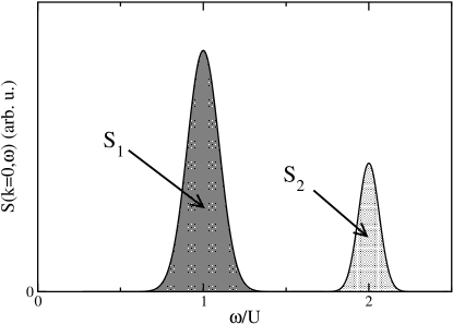
Figure 4: Sketch of the distribution of spectral weight $S(k=0,\omega)$. The weight centered around $\omega=U$ is given by $S_{1}$, the weight around $\omega=2U$ by $S_{2}$.

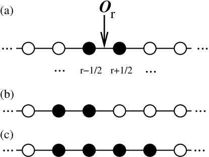
Figure 5: Terms of the local observable $R(l,{\mathbf{r}})$. The arrow indicates the bond on which a term acts. Filled circles: sites on which a non-trivial operator acts; ‘non-trivial’ means that the operator is different from the identity. Open circles: sites on which the term under study does not act, i.e., the term acts as identity on these sites. (a) At $l=0$ the observable is $H_{t}$. It is composed of local terms that act only on adjacent sites of the lattice. (b) and (c) More complicated terms appear during the flow. The sum of the distances of all operators in a term is our measure $r_{\mathcal{O}}$ for the extension of a term. It is $2$ for (b) and $4$ for (c). Terms beyond a certain extension are omitted.

We compute the matrix elements of the excitation operator after the CUT, i.e., of ${R}^{\rm eff}$. This operator consists of terms of the form $c_{(\bar{n};\bar{m})}(h^{\dagger})^{n_{h}}(p^{\dagger})^{n_{p}}(d^{\dagger})^{n_{d}}h^{m_{h}}p^{m_{p}}d^{m_{d}}$ where we omitted all spatial subscripts denoting only the powers $(\bar{n};\bar{m})=(n_{h}\;n_{p}\;n_{d};m_{h}\;m_{p}\;m_{d})$ of the particular operator type. For the full expression we refer the reader to Appendix A. The coefficient $c_{(\bar{n};\bar{m})}$ is the corresponding prefactor. The spectral weight $I^{\text{eff}}_{(\bar{n};\bar{m})}$ is the integral of $S(k=0,\omega)$ over all frequencies for momentum transfer $k=0$. It stands for the excitation process starting from the states with $m_{d}$ double-particles, $m_{p}$ particles, and $m_{h}$ holes and leading to the states with $n_{d}$ double-particles, $n_{p}$ particles, and $n_{h}$ holes.

In the course of the flow, contributions to the observable appear which do not act on the bond on which the initial observable is centered. The initial local process spreads out in real space for $l\to\infty$. Examples are sketched in Fig. 5b-c. In order to avoid proliferation, also the terms in the observable have to be truncated. Like for the terms in the Hamiltonian we introduce a measure for the extension of the terms in the observable. This measure, however, is slightly different: It is the sum $r_{\mathcal{O}}$ of the distances of all its local creation or annihilation operators to ${\mathbf{r}}$. If the value $r_{\mathcal{O}}$ of a certain term exceeds a preset truncation criterion, this term is neglected.

Figures 5b-c illustrate the truncation criterion for the observable. An operator that acts on the sites shown in Figure 5b meets the truncation criterion for $r_{\mathcal{O}}=3$. It is kept in a $r_{\mathcal{O}}=3$ calculation. An operator acting on the sites in Figure 5c is kept in the calculation with $r_{\mathcal{O}}=4$. But it does not meet the truncation criterion for $r_{\mathcal{O}}=3$; in a calculation with $r_{\mathcal{O}}=3$ it is discarded.

Once the local effective observables $R(l=\infty,{\mathbf{r}})$ are known, the total effective expression $R^{\text{eff}}$ is given by the sum over all bonds (7).

Figure 6: (color online) Spectral weights of various processes for truncations $r_{\mathcal{O}}\in\{2,3,4\}$. (a) $I^{\text{eff}}_{(\text{hp;0})}$ (black curves) and $I^{\text{eff}}_{(2\text{h2p};0)}$ (green/grey). (b) $I^{\text{eff}}_{(\text{h2p;p})}+I^{\text{eff}}_{(\text{2hp;h})}$ (black) and $I^{\text{eff}}_{(\text{hd;p})}$ (green/grey)

The results for the observable truncations $r_{\mathcal{O}}\in\{2,3,4\}$ are shown in Fig. 6. At zero temperature, only the processes starting from the ground state are relevant. These processes are the $(\bar{n};0)$ processes which start from the reference state $|\text{ref}\rangle$ because the CUT is constructed such that the reference state, which is the vacuum of excitations, becomes the ground state after the transformation Knetter and Uhrig (2000); Mielke (1998); Knetter et al. (2003). The weights of the $(\bar{n};0)$ processes are shown in Fig. 6a. The by far dominant weight is $I^{\text{eff}}_{(\text{hp};0)}$; the process $I^{\text{eff}}_{(\text{2h2p};0)}$ is lower by orders of magnitude. The agreement between results for various truncations is very good.

The particle-hole pair excited in $I^{\text{eff}}_{(\text{hp};0)}$ has about the energy $U$ for low values of $t/U$, while $I^{\text{eff}}_{(\text{2h2p};0)}$ leads to a response at $2U$. Hence we find noticeable weight only around $U$ in accordance with recent quantum Monte Carlo (QMC) data Batrouni et al. (2005).

At finite temperature, excitations are present before $R^{\text{eff}}$ is applied. At not too high temperatures, independent particles $p^{\dagger}$ and holes $h^{\dagger}$ are the prevailing excitations. Other excitations, for instance $d^{\dagger}$ or correlated states $(p^{\dagger})^{2}$ of two $p$-particles, are higher in energy and thus much less likely. So the processes starting from a particle or a hole are the important ones which come into play for $T>0$. Hence we focus on $I^{\text{eff}}_{(\text{h2p;p})}$, $I^{\text{eff}}_{(\text{2hp;h})}$, and $I^{\text{eff}}_{(\text{hd;p})}$. These weights are shown in Fig. 6b. The results for $I^{\text{eff}}_{(\text{hd;p})}$ depend only very little on truncation. A larger dependence on the truncation is found for $I^{\text{eff}}_{(\text{h2p;p})}+I^{\text{eff}}_{(\text{2hp;h})}$. But the agreement is still satisfactory.

The processes $I^{\text{eff}}_{(\text{h2p;p})}$ and $I^{\text{eff}}_{(\text{2hp;h})}$ increase the energy by about $U$ because they create an additional particle-hole pair. The $I^{\text{eff}}_{(\text{hd;p})}$ process increments the energy by about $2U$ because a hole and a double-particle is generated.

V Approaching Experiment

Let us address the question what causes the high energy peak in Refs. Greiner et al. (2002); Stöferle et al. (2004); Köhl et al. (2005). It was suggested that certain defects, namely an adjacent pair of a singly and a doubly occupied site, are at the origin of the high energy peak. The weight of such processes for a given particle state is quantified by $I^{\text{eff}}_{(\text{hd;p})}$. Its relatively high value, see Fig. 6b, puts the presumption that such defects cause the peak at $2U$ on a quantitative basis.

V.1 Zero Temperature

But what generates such defects? At zero or at very low temperature, the inhomogeneity of the parabolic trap can imply the existence of plateaus of various occupations $\langle n\rangle\in\{0,1,2,\ldots\}$ depending on the total filling Batrouni et al. (2002); Kollath et al. (2004); Batrouni et al. (2005). In the transition region from one integer value of $\langle n\rangle$ to the next, defects occur which lead to excitations at $2U$.

Yet it is unlikely that this mechanism explains the experimental finding since the transition region is fairly short at low value of $T/U$ and $t/U$, i.e., the plateaus prevail. The high energy peak at $2U$, however, has less weight by only a factor $2$ to $5$ compared to the weight in the low energy peak at $U$ Stöferle et al. (2004). So we conclude that the inhomogeneity of the traps alone cannot be sufficient to account for the experimental findings.

V.2 Finite Temperature

At higher temperatures, thermal fluctuations are a likely candidate for the origin of the defects. Hence we estimate their effect in the following way. Thermally induced triply occupied $d$ states are neglected because they are very rare due to their high energy of $\omega^{\text{d}}(k)-2\mu\approx 2U$ above the vacuum $|\text{ref}\rangle$. We focus on the particle $p$ and the holes $h$. The average occupation of these states is estimated by a previously introduced approximate hardcore boson statistics Troyer et al. (1994)

$$\langle n^{\sigma}_{k}\rangle = \exp\left({-\beta(\omega^{\sigma}(k)-\mu^{\sigma})}\right)\langle n^{\rm vac}\rangle$$ (8a)

$$\langle n^{\rm vac}\rangle = \left(1+z^{\rm p}(\beta)+z^{\rm h}(\beta)\right)^{-1}\ ,$$ (8b)

where $z^{\sigma}=(2\pi)^{-1}\int_{0}^{2\pi}dke^{-\beta(\omega^{\sigma}(k)-\mu^{\sigma})}$, $\mu=\mu^{\text{p}}=-\mu^{\text{h}}$. The chemical potential changes sign for the holes because a hole stands for the absence of one of the original bosons $b$. Equation (8) is obtained from the statistics of bosons without any interaction by correcting globally for the overcounting of states. The fact that the overcounting is remedied on an average level implies that (8) represents only an approximate, classical description Schmidt et al. (2005). The chemical potential $\mu$ is determined self-consistently such that as many particles as holes are excited, i.e., the average number of bosons $b$ per site remains one.

Figure 7: (color online) Temperature dependence of the relative spectral weight $S_{2}/S_{1}$ for various values of $t/U$. Inset: $S_{2}/S_{1}$ as function of $t/U$ for various temperatures.

Next, we turn to the computation of spectral weights at finite temperatures. At not too high temperatures, the relevant channels are $(\text{hp};0)$, $(\text{h2p;p})$, $(\text{2hp;h})$, which excite at around $U$ and $(\text{2h2p};0)$, $(\text{hd;p})$, which excite at around $2U$. The spectral weights at finite $T$ are calculated by Fermis golden rule as before. The essential additional ingredient is the probability to find a particle, or a hole, respectively, to start from and to find sites which can be excited, i.e., which are not occupied by a particle or a hole. This leads us to the equations

$$I^{\text{eff},T}_{(\bar{n};0)} = I^{\rm eff}_{(\bar{n};0)}\langle n^{\rm vac}\rangle^{n_{h}+n_{p}+n_{d}}$$ (9a)

$$I^{\text{eff},T}_{(\bar{n};\sigma)} = \frac{\langle n^{\rm vac}\rangle^{n_{h}+n_{p}+n_{d}}}{2\pi}\int_{0}^{2\pi}I^{k,{\rm eff}}_{(\bar{n};\sigma)}\langle n^{\sigma}_{k}\rangle dk$$ (9b)

with $\sigma\in\{\text{p,h}\}$. The powers of $\langle n^{\rm vac}\rangle$ account for the probability that the sites to be excited are not blocked by other excitations; the factor $\langle n^{\sigma}_{k}\rangle$ accounts for the probability that the excitation necessary for the particular process is present. The momentum dependence in $I^{k,{\rm eff}}$ stems from the momentum dependence of the annihilated particle or hole. It is computed by the sum of the moduli squared of the Fourier transform of the matrix elements $c_{(\bar{n};\bar{m})}$ in the real space coordinate of the annihilated excitation.

The spectral weight in the high energy peak (at $2U$) relative to the weight in the low energy peak (at $U$) is given by the ratio $S_{2}/S_{1}$ where $S_{2}=I^{\text{eff},T}_{(\text{2h2p};0)}+I^{\text{eff},T}_{(\text{hd;p})}$ and $S_{1}=I^{\text{eff},T}_{(\text{hp};0)}+I^{\text{eff},T}_{(\text{h2p;p})}+I^{\text{eff},T}_{(\text{2hp;h})}$. Fig. 7 displays this key quantity as function of $t/U$ and $T/U$ for $r_{\mathcal{O}}=4$. The difference to the result for $r_{\mathcal{O}}=3$ is less than $0.005$.

Two regimes can be distinguished. For low values of $T\lessapprox 0.19U$, the ratio $S_{2}/S_{1}$ increases on increasing $t/U$ because the particle gap $\Delta^{\text{p}}$ decreases so that $\langle n^{\text{p}}_{k\approx 0}\rangle$ grows. For higher values of $T\gtrapprox 0.19U$, the increase of $\langle n^{\text{p}}_{k\approx 0}\rangle$ is overcompensated by the decrease of the weights $I^{\text{eff},T}_{(\text{2h2p};0)}+I^{\text{eff},T}_{(\text{hd;p})}$ and the increase of the weights $I^{\text{eff},T}_{(\text{hp};0)}+I^{\text{eff},T}_{(\text{h2p;p})}+I^{\text{eff},T}_{(\text{2hp;h})}$, cf. Fig. 6, so that the relative spectral weight decreases on increasing $t/U$. Around $T=0.19U$, the ratio is fairly independent of $t/U$.

The experimental value of $S_{2}/S_{1}$ Stöferle et al. (2004) is about $0.2-0.5$ for small values of $t/U$ ($t\leq 0.03U$). It increases on approaching the superfluid phase. Hence, our estimate for $S_{2}/S_{1}$ implies a significant temperature $T\approx U/3$ in the MI phase, which was not expected. This is the main result of our analysis of the spectral weights.

VI Discussion

The analysis of the spectral weights lead us to the conclusion that the temperature of the Mott-insulating phases must be quite considerable. At first sight, this comes as a surprise because other experiments on cold atoms imply very low temperatures, see for instance Ref. Paredes et al., 2004. But the seeming contradiction can be resolved.

One has to consider the entropies involved Blakie and Porto (2004); Rey (2004). The entropy per boson $S/N$ in a three-dimensional harmonic trap is given by $\approx 3.6(1-f_{0})$ where $f_{0}$ is the fraction of the Bose-Einstein condensate Schmidt et al. (2005). Adiabatic loading into the optical lattice keeps $S/N$ constant so that we can estimate the temperature of the MI phase from the derivative of the free energy Troyer et al. (1994). For $f_{0}=0.95;0.9;0.8$ we obtain significant temperatures $T/U=0.12;0.17;0.27$ in satisfactory agreement with the analysis of the spectral weights Schmidt et al. (2005). The analogous estimate in the case of the Tonks-Girardeau limit (large $U$ and average filling $n$ below unity, see Ref. Paredes et al., 2004) leads to temperatures of the order of the hopping $t$: $T/t=0.17;0.32;0.61$ (assuming $n=1/2$) Schmidt et al. (2005). These values are again in good agreement with experiment.

The physical interpretation is the following. On approaching the Mott insulator by changing the filling to the commensurate value $n\to 1$ the temperature has to rise because the available phase space decreases. For $n<1$ there is phase space without occupying any site with two or more bosons $b$ because one can choose between occupation 0 or 1. But at $n=1$ the state without any doubly occupied site is unique. Hence no entropy can be generated without inducing doubly occupied and empty sites, i.e., excitations of $p$- and of $h$-type. This in turn requires that the temperature is of the order of the gap which agrees well with our analysis of the spectral weights.

We like to draw the reader’s attention to the fact that our result of a fairly large temperature ($T\approx U/3$) provides also a possible explanation why no response at $\approx 2U$ was found by QMC a low temperatures Batrouni et al. (2005). Further investigations will be certainly fruitful, e.g., it would be interesting to obtain QMC results for the excitation operator $R$ that we used in our present work. The excitation operator used in Ref. Batrouni et al., 2005 vanishes for vanishing momentum so that it is less suited to describe the experimental Bragg spectroscopy Stöferle et al. (2004).

In the attempt to provide quantitive numbers for the temperature in the MI bose systems one must be cautious because the bosonic systems are shaken fairly strongly in experiment Stöferle et al. (2004); Köhl et al. (2005). Though it was ascertained that the experiment was conducted in the linear regime it might be that the systems are heated by the probe procedure so that the temperatures seen in the spectroscopic investigations are higher than those seen by other experimental investigations.

It would be rewarding to clarify the precision of the spectroscopic investigations. Then the pronounced $T$ dependence of the relative spectral weight in Fig. 7 could be used as a thermometer for Mott-insulating bosons in optical lattices.

In summary, we have studied spectral properties of bosons in one-dimensional optical lattices using particle-conserving continuous unitary transformations (CUTs). At $T=0$ and for small $t/U$ spectral weight is only present at energies $\approx U$. Recent experimental peaks at $\approx 2U$ Stöferle et al. (2004) can be explained assuming $T\approx U/3$. Our results suggest to investigate the effects of finite $T$ on bosons in optical lattices much more thoroughly.

Appendix A Explicit expression for the observable

The local observable depending on the flow parameter $l$ reads

$$R(l,\mathbf{r}) = \sum_{\{i,i^{\prime},j,j^{\prime},k,k^{\prime}\}}c(l,\{i,i^{\prime},j,j^{\prime},k,k^{\prime}\})\times$$

$$\quad h_{i_{1}+r}^{\dagger}\cdot...\cdot h_{i_{n_{h}}+r}^{\dagger}h_{i^{\prime}_{1}+r}^{\phantom{\dagger}}\cdot...\cdot h_{i^{\prime}_{m_{h}}+r}^{\phantom{\dagger}}\times$$

$$\quad p_{j_{1}+r}^{\dagger}\cdot...\cdot p_{j_{n_{p}}+r}^{\dagger}p_{j^{\prime}_{1}+r}^{\phantom{\dagger}}\cdot...\cdot p_{j^{\prime}_{m_{p}}+r}^{\phantom{\dagger}}\times$$

$$\quad d_{k_{1}+r}^{\dagger}\cdot...\cdot d_{k_{n_{d}}+r}^{\dagger}d_{k^{\prime}_{1}+r}^{\phantom{\dagger}}\cdot...\cdot d_{k^{\prime}_{m_{d}}+r}^{\phantom{\dagger}}.$$

The numbers $(n_{h}\;n_{p}\;n_{d};m_{h}\;m_{p}\;m_{d})$ are defined as the number of operators involved in a term in Eq. A. The number of creation operators $h^{\dagger}$, $p^{\dagger}$, and $d^{\dagger}$ is given by $n_{h}$, $n_{p}$, and $n_{d}$, respectively. The number of annihilation operators $h$, $p$, and $d$ is given by $m_{h}$, $m_{p}$, and $m_{d}$, respectively. A set of these six numbers defines the type $(\bar{n};\bar{m})$ of a process. The variables $\{i,i^{\prime},j,j^{\prime},k,k^{\prime}\}$ are multi-indices, e. g. $i=\{i_{1},...,i_{n_{h}}\}$ which give the position of the operator. The coefficients $c(l,\{i,i^{\prime},j,j^{\prime},k,k^{\prime}\})$ keep track of the amplitudes of these processes during the flow. Their value at $l=\infty$ defines the effective observable $R^{\text{eff}}$.

The total observable is the sum

$$R(l)=\sum_{{\mathbf{r}}}R(l,{\mathbf{r}}).$$ (11)

No phase factors occur so that the observable is invariant with respect to translations. Hence no momentum transfer takes place and the response at $k=0$ is the relevant one.

References

- Greiner et al. (2002) M. Greiner, O. Mandel, T. W. Hänsch, and I. Bloch, Nature 419, 51 (2002).
- Paredes et al. (2004) B. Paredes, A. Widera, V. Murg, O. Mandel, S. Fölling, I. Cirac, G. V. Shlyapnikov, T. W. Hänsch, and I. Bloch, Nature 429, 277 (2004).
- Stöferle et al. (2004) T. Stöferle, H. Moritz, C. Schori, M. Köhl, and T. Esslinger, Phys. Rev. Lett. 92, 130403 (2004).
- Köhl et al. (2005) M. Köhl, H. Moritz, T. Stöferle, C. Schori, and T. Esslinger, J. Low Temp. Phys. 138, 635 (2005).
- Jaksch et al. (1998) D. Jaksch, C. Bruder, J. I. Cirac, C. W. Gardiner, and P. Zoller, Phys. Rev. Lett. 81, 3108 (1998).
- Fisher et al. (1989) M. P. A. Fisher, P. B. Weichman, G. Grinstein, and D. S. Fisher, Phys. Rev. B 40, 546 (1989).
- Pai et al. (1996) R. V. Pai, R. Pandit, H. R. Krishnamurthy, and S. Ramasesha, Phys. Rev. Lett. 76, 2937 (1996).
- Kashurnikov and Svistunov (1996) V. A. Kashurnikov and B. V. Svistunov, Phys. Rev. B 53, 11776 (1996).
- Kühner and Monien (1998) T. D. Kühner and H. Monien, Phys. Rev. B 58, R14741 (1998).
- Elstner and Monien (1999) N. Elstner and H. Monien, Phys. Rev. B 59, 12184 (1999).
- Kühner et al. (2000) T. D. Kühner, S. R. White, and H. Monien, Phys. Rev. B 61, 12474 (2000).
- Batrouni et al. (2005) G. G. Batrouni, F. F. Assaad, R. T. Scalettar, P. J. H. Denteneer, and M. Troyer, cond-mat/0503371 (2005).
- Wegner (1994) F. J. Wegner, Ann. Physik 3, 77 (1994).
- Knetter and Uhrig (2000) C. Knetter and G. S. Uhrig, Eur. Phys. J. B 13, 209 (2000).
- Knetter et al. (2003) C. Knetter, K. P. Schmidt, and G. S. Uhrig, J. Phys. A: Math. Gen. 36, 7889 (2003).
- Reischl et al. (2004) A. Reischl, E. Müller-Hartmann, and G. S. Uhrig, Phys. Rev. B 70, 245124 (2004).
- Schmidt and Uhrig (2005) K. P. Schmidt and G. S. Uhrig, in preparation (2005).
- Mielke (1998) A. Mielke, Eur. Phys. J. B 5, 605 (1998).
- Batrouni et al. (2002) G. G. Batrouni, V. Rousseau, R. T. Scalettar, M. Rigol, A. Muramatsu, P. J. H. Denteneer, and M. Troyer, Phys. Rev. Lett. 89, 117203 (2002).
- Kollath et al. (2004) C. Kollath, U. Schollwöck, J. von Delft, and W. Zwerger, Phys. Rev. A 69, 031601(R) (2004).
- Troyer et al. (1994) M. Troyer, H. Tsunetsugu, and D. Würtz, Phys. Rev. B 50, 13515 (1994).
- Schmidt et al. (2005) K. P. Schmidt, A. Reischl, and G. S. Uhrig, in preparation (2005).
- Blakie and Porto (2004) P. B. Blakie and J. V. Porto, Phys. Rev. A 69, 013603 (2004).
- Rey (2004) A. M. Rey, Ultracold bosonic atoms in optical lattices (PhD thesis, University of Maryland, College Park, USA, 2004).