Transport of atoms in a quantum conveyor belt

Abstract

We have performed experiments using a 3D-Bose-Einstein condensate of sodium atoms in a 1D optical lattice to explore some unusual properties of band-structure. In particular, we investigate the loading of a condensate into a moving lattice and find non-intuitive behavior. We also revisit the behavior of atoms, prepared in a single quasimomentum state, in an accelerating lattice. We generalize this study to a cloud whose atoms have a large quasimomentum spread, and show that the cloud behaves differently from atoms in a single Bloch state. Finally, we compare our findings with recent experiments performed with fermions in an optical lattice.

An optical lattice is a practically perfect periodic potential for atoms, produced by the interference of two or more laser beams. An atomic-gas Bose-Einstein condensate (BEC)Anderson ; dafolvo99 is a coherent source of matter waves, a collection of atoms, all in the same state, with an extremely narrow momentum spread. Putting such atoms into such a potential provides an opportunity for exploring a quantum system with many similarities to electrons in a solid state crystal but with unprecedented control over both the lattice and the particles. In particular we can easily control the velocity and acceleration of the lattice as well as its strength, making it a variable “quantum conveyor belt”. This allows us to explore situations that are difficult or impossible to achieve in solid state systems. The results are often remarkable and counter-intuitive. For example atoms that are being carried along by a moving optical lattice are left stationary when the still-moving lattice is turned off, in apparent violation of the law of inertia.

A few experiments have studied quantum degenerate atoms in moving optical lattices Fallani03 ; Morsch01 ; Eiermann03 ; Denschlag02 . Bragg diffraction of a Bose condensate is a special case of quantum degenerate atoms in a moving lattice Kozuma99 . Here, using a Bose-Einstein condensate and a moving lattice, we achieve full control over the system, in particular its initial quasimomentum and band index as well as its subsequent evolution. We also show the difference in behavior when the atom sample has a large spread of quasimomenta, as compared with the narrow quasimomentum distribution of a coherent BEC.

Our lattice is one-dimensional along the $x$ axis, produced by the interference of two counter-propagating laser beams, each of wave-vector $k=2\pi/\lambda$ ($\lambda\approx 589$ nm is the wavelength of the laser beams). This results in a sinusoidal potential, $V\sin^{2}kx$, with a spatial period $\lambda/2$.

We will use Bloch theory, emphasizing the single particle character of the problem. An overview of Bloch theory, as it applies to this one dimensional system, is supplied in reference Denschlag02 . Briefly, the wave function of the atoms in the lattice can be decomposed into the Bloch eigenstates $u_{n,q}(x)e^{iqx}$ characterized by a band index $n$ and a quasimomentum $q$, defined in the rest frame of the lattice. The eigenenergies of the system, $E_{n}(q)$, as well as the eigenstates are periodic in $q$ with a periodicity $2\mbox{$\hbar k$}$, the reciprocal lattice vector of the lattice. A wave packet in band $n$ with quasimomentum distribution centered at $q$, has a group velocity $\mbox{$v_{\rm g}$}=dE_{n}(q)/dq$. Fig. 1 shows the band structure in the repeated-zone scheme Ashcroft , for a lattice with a depth $V=4\mbox{$E_{\rm r}$}$ ($E_{\rm r}$ is the single-photon recoil energy given by $\mbox{$E_{\rm r}$}=\hbar^{2}k^{2}/2M$ and is related to the recoil velocity $v_{\rm r}$ by $\mbox{$v_{\rm r}$}=M\mbox{$v_{\rm r}$}^{2}/2$, $M$ being the mass of an atom). Note that for convenience the band-energies $E_{n}$ are offset such that they coincide at large band index with the free parabolae; this shows more clearly the avoided crossings between free particle states due to the laser-induced coupling. These avoided crossings create the band gaps that separate energy bands with different indices $n$.

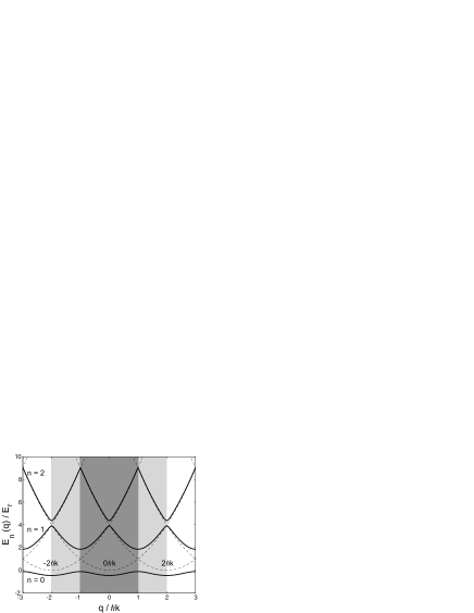
Figure 1: Band structure for a 4$E_{\rm r}$ deep lattice in the repeated-zone scheme. The dotted lines represent the free particle parabolae to which the bands adiabatically connect as $V\rightarrow 0$. The region in dark grey corresponds to the first Brillouin zone. The region in light grey corresponds to the second Brillouin zone.

I Experimental setup

The experimental setup has been described previously Kozuma99 . An almost pure Bose-Einstein condensate (no discernable thermal component) of about $2\times 10^{6}$ sodium atoms is prepared in a triaxial Time Orbiting Potential (TOP) trap Petrich95 ; Kozuma99 . We adiabatically expand the condensate by lowering the mean trapping frequency from 200 Hz to a value ranging from 100 Hz to 19 Hz. This reduces the atom-atom interaction, the strength of which is given by the chemical potential $\mu=\frac{4\pi\hbar^{2}na}{M}$ dafolvo99 , $n$ being the density at the center of the cloud and $a\approx 2.8$ nm the scattering length. During the expansion, the calculated Thomas-Fermi diameter, $2R$, of the condensate along the lattice direction increases from 18 $\mu\mathrm{m}$ up to values ranging from 24 $\mu\mathrm{m}$ to 48 $\mu\mathrm{m}$. The wave-function of each atom thus covers more than a 100 lattice sites and is an excellent approximation of a Bloch state. The rms width of the momentum distribution of the atoms in the condensate along the axis of the lattice is $\sqrt{3}\,\hbar/R$ Stenger99 . Therefore the rms width of the quasimomentum distribution of each atom is $\Delta q\sim(\lambda/4R)\ \mbox{$\hbar k$}\leq 0.01\mbox{$\hbar k$}$.

To form the lattice we use two counter-propagating laser beams perpendicular to gravity. Each has a power of up to 10 mW and is detuned either 200-350 GHz to the blue of the sodium D2 transition (experiments of sections II and IV) or 700 GHz to the red of the D1 transition (last section). They are focused to a beam waist of about 200 $\mu$m FWHM, leading to a calculated spontaneous emission rate $\leq 30\ \rm{s}^{-1}$, negligible during the time of the experiments. The lattice depth, measured by observing the Bragg diffraction Denschlag02 , is up to 13$E_{\rm r}$. We use acousto-optic modulators to independently control the frequencies and intensities of the beams. The unmodulated intensity is kept constant to within 5% by active stabilization. A frequency difference $\delta$ between the two beams produces a “moving standing wave” of velocity $v=\delta/2k$. Numerically, a difference of $\delta/2\pi=100$ kHz corresponds to a lattice velocity of one recoil velocity, $\mbox{$v_{\rm r}$}=\mbox{$\hbar k$}/M\approx 3$ cm/s.

The cloud’s momentum is analyzed using time-of-flight. The time-of-flight period, typically a few milliseconds, converts the initial momentum distribution into a position distribution, which we determine using near-resonance absorption imaging along an axis perpendicular to the axis of the lattice.

II Dragging a condensate in a moving lattice

In a first set of experiments, we begin with a BEC in a magnetic trap with a 19 Hz mean frequency. This weak trap makes the interactions between atoms almost negligible on the time scale of the experiment, i.e. $\hbar/\mu$ is generally longer than the duration of the experiment . After turning off the magnetic trap, we adiabatically apply a moving lattice with a final depth of 4$E_{\rm r}$. The turn-on time of the lattice intensity is 200 $\mu$s, an interval chosen to ensure adiabaticity with respect to band excitation  (see section III). The fixed velocity of the lattice, $v$, is between 0 and about 3$v_{\rm r}$. In the lattice frame the atoms have a quasimomentum $q=-Mv$. Because the width of the quasimomentum distribution is very narrow, this procedure produces a good approximation of a single Bloch state with a freely chosen $q$.

Atoms loaded in this way are dragged along with the moving lattice. In the limit that the lattice is very deep so that the bands are flat (i.e. $\frac{dE(q)}{dq}=0$), the group velocity with respect to the lattice, $v_{\rm g}$, is 0 and the atoms are dragged in the lab frame at the velocity of the lattice. For finite depth lattices the dragging velocity in the lab frame is $v+\mbox{$v_{\rm g}$}$. (Note that for $v>0$, $\mbox{$v_{\rm g}$}<0$ so that this dragging velocity in the lab frame $v+\mbox{$v_{\rm g}$}\leq v$.)

In order to experimentally measure the dragging velocity we suddenly (on the order of $200$ ns) turn off the moving lattice, projecting the Bloch state onto the basis of free-particle momentum eigenstates while preserving the momentum distribution. Figure 2a shows the lattice depth as a function of time. Images of the resulting diffraction pattern for various lattice velocities are presented in figure 2b.

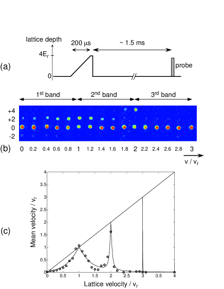
Figure 2: (Color) Dragging of atoms in a moving lattice followed by a sudden turn-off of the lattice. Fig. 2a presents the time sequence. Fig.  2b shows the absorption image of the cloud after a 1.5 ms time of flight following a sudden turn off of the lattice for different lattice velocities $v$, related to the quasimomentum by $q=-Mv$. The numbers on the vertical axis refer to the atomic velocity in units of $v_{\rm r}$. The average velocity of the atoms in the lab frame, deduced from fig. 2b, is shown in fig. 2c versus the velocity of the lattice. The initial velocity of the condensate in the magnetic trap fluctuates with an RMS value of 0.03$v_{\rm r}$. The mean velocity, after suddenly turning off the lattice, thus exhibits the same fluctuations. The solid curve is the mean velocity of the atoms calculated from the band structure for a 4$E_{\rm r}$ deep lattice.

The average velocity seen from the diffraction pattern (the weighted average of the velocities of the individual diffraction components) increases with the lattice velocity through the first Brillouin zone. In fact for this rather flat band the dragging velocity is roughly equal to the lattice velocity. (The details for higher velocities are discussed in the following section.)

An alternate method to study the atomic momentum is to release the condensate adiabatically ($\sim 200\ \mu$s) rather than suddenly, thus avoiding diffraction. Figure 3a shows the lattice intensity time sequence for this method. The corresponding images for various lattice velocities appear in figure 3b.

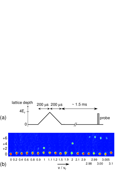
Figure 3: (Color) Dragging of atoms in a moving lattice followed by an adiabatic turn-off of the lattice. Fig. 3a presents the time sequence. Fig. 3b shows the absorption image of the cloud after a 1.5 ms time of flight following the adiabatic turn-off of the lattice for different lattice velocities. The numbers on the vertical axis refer to the atomic velocity in units of $v_{\rm r}$.

These pictures show that (apart from when the lattice velocity is very close to an integer multiple of $v_{\rm r}$, a situation discussed in section III) the atoms are back at rest in the laboratory frame, despite the fact that the lattice is still moving during the ramping down of its intensity. This is true even in the first Brillouin zone where the lattice drags the condensate at roughly the lattice velocity. This result is especially surprising when one considers that atoms moving with the lattice return to zero velocity as if they had no inertia. One might also ask how do the dragged atoms “know” that they should be at rest when the lattice is turned off. One way of understanding this is to note that the lattice turns on adiabatically and turns off adiabatically along the same path. This must necessarily return an eigenstate of the hamiltonian to the same eigenstate. A more detailed explanation involving band-structure will be presented in the next section.

III Analysis of the experiments

All experiments described in this paper start with an adiabatic turn-on of a lattice moving at a velocity $v$. In the lattice frame, in the limit of a vanishingly small lattice depth, the atomic wavefunction of a momentum eigenstate has a phase gradient $-Mv/\hbar$ corresponding to the velocity $-v$ of the atoms with respect to the lattice. This free particle state is also a Bloch state with a quasimomentum $q$ corresponding to a phase gradient $q/\hbar$, so that $q=-Mv$. All changes in the lattice intensity preserve this quasimomentum (as can be seen by calculating that the matrix elements of the periodic potential between Bloch states of different $q$, are zero). When the lattice is fully turned on, the quasimomentum is still $-Mv$ and if the turn-on has been adiabatic (so that no change in band index occurs), we end up in a single Bloch state.

Referring to figure 1 we see that, when atoms are loaded adiabatically into the lattice with the quasimomentum in the first Brillouin zone, the free particle momentum connects to the corresponding quasimomentum in the lowest, $n=0$, band. For quasimomenta outside the first Brillouin zone, the free particle momenta connect to the corresponding quasimomenta in the appropriate band. For example if the velocity of the lattice is $1.5\mbox{$v_{\rm r}$}$, i.e. in the second Brillouin zone, the atoms will end up in the second, $n=1$, band with a quasimomentum $q=-1.5\hbar k$. There is thus a strict relation between the range of quasimomenta and the band index into which the atoms are loaded: if the quasimomentum is in the $n^{\rm th}$ Brillouin zone, the atoms are loaded into band $n-1$. On the other hand, if for example we wish to prepare the atoms in $q=-1.5\hbar k$ and $n=0$, we would have to accelerate the lattice, as described in section IV.

The condition for adiabaticity with respect to band excitation during the loading has been detailed in ref.Denschlag02 : in order to avoid transitions from a given band to an adjacent band, the rate of change of the lattice depth $V$ must fulfill $\frac{dV}{dt}|\langle n,q|\sin^{2}kx|n\pm 1,q\rangle|\ll\Delta E^{2}/\hbar$. $\Delta E$ is the energy difference between the given band and its nearest neighbor. When $\Delta E$ approaches 0 (as is usually the case near a Brillouin zone boundary when $V\rightarrow 0$) the process cannot be adiabatic. For $q=0,n=0$, $\Delta E\geq 4\mbox{$E_{\rm r}$}$, and the natural time scale for adiabaticity with respect to band excitation is on the order of $h/4\mbox{$E_{\rm r}$}$. We emphasize that in the limit of $V\rightarrow 0$ there is a natural energy gap due to the periodicity of the lattice, $\Delta E\neq 0$ (except at the edge of the Brillouin zones). The existence of this non-zero energy gap when the lattice depth goes to zero is in contrast to, for example, a harmonic oscillator for which the spacing between energy levels does go to zero as the strength of the potential vanishes.

We now analyze in more detail the two methods for studying the momentum distribution described in the previous section.

In the first method we turn off the lattice potential suddenly, i.e. diabatically. This sudden turn-off leaves the atomic momentum distribution unchanged from what it was in the lattice. If the atoms are in a Bloch state, corresponding to a single value of $q$, the wave-function as viewed in the rest frame of the lattice is a superposition of plane waves with momenta $q+2m\hbar k$ ($m$ is an integer). The population-weighted average of the momentum components gives the mean momentum of the atoms in the lattice, which is $M\mbox{$v_{\rm g}$}$ Ashcroft . In the laboratory frame these momentum components are shifted by the velocity of the lattice and are observed as a diffraction pattern. The time-of-flight spatial distribution of these momentum components is analogous to the diffraction pattern of any wave from a periodic structure. The spacing between the momentum components gives the reciprocal lattice vector, 2$\hbar k$ in our case. This diffraction is characteristic of sudden turn-off (or on) of the lattice.

Figure 2c shows the measured dragging velocity in the lab frame as a function of the lattice velocity $v=-q/M$. Also shown is the calculated dragging velocity $\frac{dE(q)}{dq}+v$ for a 4$E_{\rm r}$ deep lattice. When the atoms are in the first Brillouin zone and in the $n=0$ band they are dragged along at close to the lattice velocity, because the $n=0$ band is nearly flat (see figure 1). The next, $n=1$, band is much less flat and the atoms are not dragged at the lattice velocity except at the edge of the Brillouin zone where $\mbox{$v_{\rm g}$}=\frac{dE(q)}{dq}$ vanishes. In the third Brillouin zone, the $n=2$ band is so close to a free particle that there is almost no dragging and experimentally we do not even see good dragging near the zone boundary at 3$v_{\rm r}$ because the feature is too narrow. This behavior is rather intuitive in that the lattice drags atoms effectively up to a velocity for which the atomic kinetic energy in the lattice frame is about equal to the lattice depth. Reference Fallani03 reported similar results, measuring the dragging velocity using the displacement of the cloud rather than diffraction. (Note that they plot the group velocity.) This dragging process is also discussed in Eiermann03 .

Now let us consider the rather counter-intuitive results obtained by adiabatically ramping off the lattice intensity. As noted earlier, turning off the lattice either adiabatically or non-adiabatically does not change the quasimomentum distribution, although it may change the momentum distribution. (This assumes that no other forces besides the lattice act on the atoms in the rest frame of the lattice. This assumption would be violated, for example, in the presence of interaction between the atoms or if the lattice were accelerated.)

Consider a single Bloch state in the lattice, as is the case in the previous section. In contrast to the sudden turn-off method described above, the multiple momentum states $q+2m\mbox{$\hbar k$}$ coalesce into a single momentum component, whatever the depth of the lattice was. Looking at figure 1, we can see that any single Bloch state $|n,q\rangle$ will adiabatically connect to a single free particle parabola, unless there is a degeneracy and adiabaticity fails. For the specific experiment described in section II, where a lattice moving at a constant velocity is turned on and off, this parabola is always the one labelled $0\mbox{$\hbar k$}$. In this case the Bloch state produced is such that the single momentum component is $p=q=-Mv$ in the frame of the lattice. Transforming into the lab frame we find the velocity of the atoms to be zero, as observed.

As an alternate explanation we recall posing the question “how do the dragged atoms ‘know’ that they should be at rest when the lattice is turned off?”. We now can see that this information is stored in the phase gradient, or the quasimomentum, which does not change as the lattice is ramped on and off. We again emphasize that, in the absence of interactions, this phase information is preserved no matter how deep the lattice was or how fast the lattice was turned on and off.

Let us now return to the failure of adiabaticity near the edge of the Brillouin zones. Referring to figure 1, consider free atoms, stationary in the lab frame, but at the edge of a Brillouin zone in the lattice rest frame, for example at $q=\mbox{$\hbar k$}$ or $q=2\mbox{$\hbar k$}$. At $q=\mbox{$\hbar k$}$ atoms will, as the lattice is turned on, be loaded into both bands $n=0$ and $n=1$; at $q=2\mbox{$\hbar k$}$ atoms will be loaded into $n=1$ and $n=2$. Upon turning off the lattice, the two populated states will each connect to two free-particle parabolae. For example at $q=\mbox{$\hbar k$}$ atoms will be in both the $0\mbox{$\hbar k$}$ and $2\mbox{$\hbar k$}$ parabolae (at $q=2\mbox{$\hbar k$}$, they will be in both $0\mbox{$\hbar k$}$ and $4\mbox{$\hbar k$}$). In the lattice frame (with the lattice off) atoms at $q=\mbox{$\hbar k$}$ in the $0\mbox{$\hbar k$}$ parabola are moving with a group velocity $+\mbox{$v_{\rm r}$}$; atoms at $q=\mbox{$\hbar k$}$ in the 2$\hbar k$ parabola are moving with a group velocity $-\mbox{$v_{\rm r}$}$. Transforming back into the lab frame, these atoms are moving at $0\mbox{$v_{\rm r}$}$ and $-2\mbox{$v_{\rm r}$}$ respectively. Similarly at $q=2\mbox{$\hbar k$}$ in the lattice frame the atoms are moving at $+2\mbox{$v_{\rm r}$}$ and $-2\mbox{$v_{\rm r}$}$, corresponding to 0 and 4$v_{\rm r}$ in the lab frame. This is exactly what is experimentally seen in figure 3b. (And it is exactly the same as first- and second-order Bragg diffraction Kozuma99 ). The fraction of population in each momentum component depends on the details of the loading and the unloading. For higher bands the adiabaticity condition becomes easier to satisfy near a band edge. Even though the band gap at the level anti-crossing at the Brillouin zone edge gets smaller for larger band index, the energy difference $\Delta E$ between adjacent bands at a fixed distance in quasimomentum from the Brillouin zone edge, is larger for higher bands (see fig. 1). This larger $\Delta E$ leads to greater adiabaticity for a given rate of change of the lattice depth at given distance in quasimomentum from the zone edge. This partially explains why so little population in non-zero momentum states is seen near the band edges for high velocities in fig. 3b. In addition the coupling between adjacent bands gets smaller for higher bands (because it represents a higher order process), as reflected by the narrowing of the band gap, and this smaller coupling further reduces the population of non-zero momentum states.

This method to analyze the quasimomentum distribution by adiabatically ramping down the amplitude of the lattice is independent of the way this distribution has been created, and thus allows the analysis of complex quasimomentum distributions. In order to understand this point, we recall that there is a unique correspondence (except at the Brillouin zone boundary) between any given Bloch state $|n,q\rangle$ in the lattice and a momentum state in the lab frame when the lattice is adiabatically turned off. For example two Bloch states with the same $q$ ($0<q<\mbox{$\hbar k$}$) in a lattice moving with a velocity $v$, but in two adjacent bands, let’s say $n=0$ and $n=1$, will connect to momentum states $q+Mv$ and $q+Mv-2\mbox{$\hbar k$}$ respectively. In the same way two Bloch states with the same band index and two different $q$’s will end up in two different momentum states. Suppose now we prepare a given quasimomentum distribution in the lattice frame, consisting of many $q$’s in many bands, and suppose we adiabatically ramp down the intensity of the lattice. If during that ramping-down time the quasimomentum distribution does not significantly evolve (e.g. under the influence of interaction, or under acceleration), the adiabaticity ensures that the population in a given state of quasimomentum $q$ in band $n$ is conserved during the process. The quasimomentum distribution is thus mapped onto a momentum distribution in the laboratory frame Kastberg95 . This method, which has also been used in reference Greiner2001 , then allows us to fully reconstruct the quasimomentum and band distribution.

We will give other examples of such mappings in the next two sections.

IV Acceleration of a condensate in a single Bloch state

In this section, we revisit the behavior of atoms under acceleration of the lattice, already studied in Morsch01 ; EarlyBlochoscillation ; Denschlag02 , using the adiabatic ramp-down analysis described in the last section. For this particular experiment, we again decrease the mean oscillation frequency of the magnetic trap to 19 Hz before turning the trap off. Starting with the condensate at rest in the lab frame, we linearly turn on the stationary lattice intensity over 40 $\mu\mathrm{s}$ in order to ensure adiabaticity. The final depth for this experiment is $V=13\mbox{$E_{\rm r}$}$. All the atoms are now approximately in the state $|n=0,q=0\rangle$. We then accelerate the lattice for 400 $\mu\mathrm{s}$ up to a given velocity $v_{\rm f}$, with a constant acceleration $a\leq 800\ \rm{m}/\rm{s}^{2}$. The quasimomentum $q$ of the atoms evolves during the acceleration according to a lattice version of “Newton’s law” $\dot{q}=-Ma$ Ashcroft . In the lattice frame this is equivalent to adding a linear potential $-Max$. Provided that $|Ma\langle 1,q|x|0,q\rangle|\ll E_{1}-E_{0}$ , there is no transition between the first two bands and the atoms stay in the lowest band. This implies that the acceleration should be smaller than $4\times 10^{4}$ m/$\rm{s}^{2}$, a condition well satisfied in our experiment. This acceleration allows us to produce any $q$ in the lowest band. We note that combined with the loading in a moving lattice described in section II we can therefore prepare the atoms in any Bloch state $|n,q\rangle$.

At the end of the acceleration period we ramp down the intensity of the lattice in 200 $\mu\mathrm{s}$, while still moving at $v_{\rm f}$. After a 1.2 ms time-of-flight we take an absorption image of the cloud. A series of pictures corresponding to different final lattice velocities is shown in fig. 4a.

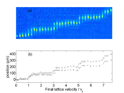
Figure 4: (Color) Acceleration of atoms in the ground state ($n=0$) band starting from $q=0$. The lattice is adiabatically raised up to $13\mbox{$E_{\rm r}$}$, accelerated and then adiabatically turned off at constant velocity. Fig. 4a shows images of the condensate after time of flight for increasing final lattice velocities. Fig. 4b shows the position of the center of mass of the cloud in the lab frame. The circles are the positions measured on fig. 4a, whereas the crosses represent the position of the cloud minus the displacement due to the dragging of the lattice. It therefore gives the momentum of the atoms.

Those pictures show that if the final lattice velocity remains within the first Brillouin zone (that is $|v_{\rm f}|<\mbox{$v_{\rm r}$}$) the cloud comes back to rest in the laboratory frame after the adiabatic ramping down of the lattice. This behavior is now well understood in light of section III. On the other hand, each time the lattice final velocity reaches $(2m+1)\mbox{$v_{\rm r}$}$ ($m$ being an integer) the atom momentum, after ramping-down the lattice, in the lab frame, increases by steps measured to be around $2\hbar k$. This momentum remains constant for any lattice velocity between $(2m+1)\mbox{$v_{\rm r}$}$ and $(2m+3)\mbox{$v_{\rm r}$}$.

As another way to understand this behavior in the first Brillouin zone, we again note that when the lattice, moving with constant speed $v_{\rm f}=-q_{\rm f}/M$, is ramped down adiabatically the velocity of the atoms with respect to the lattice varies from $\frac{dE_{0}}{dq}(q_{\rm f})$ to $q_{\rm f}/M$ when the depth of the lattice goes to 0. The velocity of the atoms in the lab frame is thus $q_{\rm f}/M+v_{\rm f}=0$.

On the other hand, if the final velocity is, say, between $v_{\rm r}$ and $3\mbox{$v_{\rm r}$}$, the velocity of the atoms in the lattice frame is no longer $q_{\rm f}/M$ after ramping down the lattice, but $(q_{\rm f}+2\mbox{$\hbar k$})/M$. For example if the lattice is accelerated to $v_{\rm f}=2.5$$v_{\rm r}$, on ramping down, the velocity in the lattice frame is $-0.5\mbox{$v_{\rm r}$}$. When the depth of the lattice approaches 0, the velocity of the cloud in the lab frame thus goes to $(q_{\rm f}+2\mbox{$\hbar k$})/M-q_{\rm f}/M=+2\mbox{$v_{\rm r}$}$. This explains the jump in momentum observed each time the velocity of the lattice reaches an odd number of recoil velocities. As in section II, the final momentum is independent of the intermediate lattice intensity. We have repeated the experiment for $V=1.5\mbox{$E_{\rm r}$}$, $5\mbox{$E_{\rm r}$}$ and $8\mbox{$E_{\rm r}$}$ and found exactly the same behavior, apart from the small non-adiabaticity at the edge of a Brillouin zone. In the case of a shallow lattice, we interpret this jump in momentum in the laboratory frame as a first order Bragg diffraction: when the velocity of the lattice reaches an odd integer multiple of $v_{\rm r}$ thus statisfying the Bragg condition, the momentum in the lab frame changes by $2\mbox{$\hbar k$}$ in the same direction as the acceleration. This Bragg diffraction is evidenced by the fact that the state of the atoms in the lattice connects to a different free parabola when the lattice is ramped down, as seen in fig. 1.

One should not be misled by the fact that the condensate is back at rest in the laboratory frame when $|v_{\rm f}|<\mbox{$v_{\rm r}$}$. The cloud has been displaced, dragged along by the lattice. The displacement is given by

$$x=\int_{0}^{\tau}\left(\frac{dE}{dq}(q(t))-q(t)/M\right)dt\ ,$$ (1)

where $\tau$ is the duration of the experiment (600 $\mu\mathrm{s}$). For lattices deeper than about $3\mbox{$E_{\rm r}$}$, the derivative almost vanishes and we approximate the displacement by $x=v_{\rm f}\,(\frac{1}{2}\tau_{\rm{accel}}+\tau_{\rm{rampdown}})$. In order to determine whether the observed jump in momentum is exactly $2\mbox{$\hbar k$}$ at the crossing of the edge of the Brillouin zone, one has to subtract this displacement due to the dragging of the lattice. This is shown in fig. 4b. The circles are the actual positions of the center of the cloud in the lab frame. The crosses represent the positions corrected by the displacement due to the dragging. The dispersion of the data on a given plateau is due to a fluctuation of the position and velocity of the condensate, with RMS values of about, respectively, 10 $\mu\mathrm{m}$ and $0.03\mbox{$v_{\rm r}$}$.

We next consider essentially the same experiment except that we now load the condensate in a lattice already moving with an initial velocity $v_{i}=-1.5\mbox{$v_{\rm r}$}$. Referring to figure 1 we see that adiabatic loading (100 $\mu$sec) prepares the atoms in the Bloch state $|n=1,q=1.5\mbox{$\hbar k$}\rangle$. When the lattice is accelerated for 400 $\mu$sec in the positive direction in the lab frame, the atoms follow the first band and the quasimomentum in the lattice frame decreases linearly with time. Figure 5a shows the position of the cloud in the lab frame after the adiabatic ramp down of the lattice (100 $\mu$sec) and the subsequent 1.2 ms time of flight. In figure 5b we show the average momentum of the cloud. This includes compensation for the dragging of the atoms during the time the lattice is on (600 $\mu$sec), as described earlier.

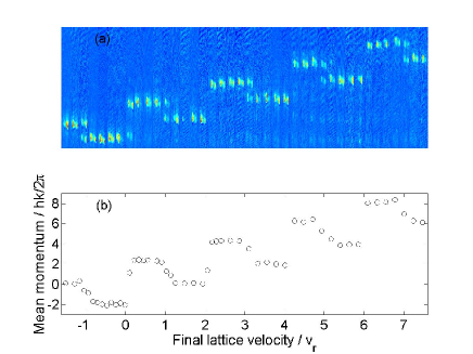
Figure 5: (Color) Acceleration of the lattice with atoms initially loaded into the band $n=1$, starting from $q=1.5\mbox{$\hbar k$}$. The 13$E_{\rm r}$ lattice is raised adiabatically, accelerated, and then turned off adiabatically. Fig. 5a shows the images of the cloud in the lab frame after a 1.2 ms time of flight for various final lattice velocities. Fig. 5b presents the momentum deduced from the positions of the cloud, after correction for the dragging.

Figure 5b shows an alternation of $-2\mbox{$\hbar k$}$ and $+4\mbox{$\hbar k$}$ momentum jumps in the lab frame. According to the interpretation in terms of Bragg diffraction, when the final velocity of the lattice reaches $-\mbox{$v_{\rm r}$}$ (or the quasimomentum reaches $+\mbox{$\hbar k$}$), the atoms undergo a first order Bragg diffraction in the direction opposite to the acceleration of the lattice in the lab (equivalently they change from the $0\mbox{$\hbar k$}$ to the $+2\mbox{$\hbar k$}$ free parabola, see figure 1). After being adiabatically released from the lattice, they now travel at $-2\mbox{$v_{\rm r}$}$ in the lab frame, in the direction opposite to the acceleration. Despite the lattice being constantly accelerated in the direction of positive momentum, at this stage the atoms gain a momentum in a direction opposite to the acceleration. Further acceleration to $v_{\rm f}=0$ leads to a second-order Bragg reflection that gives an impulse of $+4\mbox{$\hbar k$}$, in the direction of the acceleration (corresponding to a change from the $+2\mbox{$\hbar k$}$ parabola to the $-2\mbox{$\hbar k$}$ parabola in the lattice frame, see fig.1). After adiabatic release the atoms’ momentum in the lab frame is $+2\mbox{$\hbar k$}$.

As a conclusion of this section, we discuss the difference between the experiments presented here and earlier experiments investigating Bloch oscillations. In reference Morsch01 , for example, using the sudden turn-off method, the authors present the variation of the mean velocity of the atoms in the lab frame, after having accelerated the lattice. Their figure 2a shows steps of amplitude $2\mbox{$v_{\rm r}$}$ (note that their $V_{\rm B}=2\mbox{$v_{\rm r}$}$). The sharpness of the steps depends on the depth of the lattice and becomes more gentle when the lattice gets deeper (see their figure 2c) and figure 13 (upper panel) of Denschlag02 ). On the other hand our figure 4b exhibits sharp steps very similar to figure 2a of Morsch01 taken with a 0.29$E_{\rm r}$ deep lattice, despite the fact we were using a 13$E_{\rm r}$ deep lattice, the same as fig. 13 of Denschlag02 . The adiabatic turn off method with any depth lattice thus produces results equivalent to the sudden turn off method using a vanishingly small lattice depth. This is because when we turn the lattice intensity off adiabatically the states connect continuously to the Bloch states for a vanishingly shallow lattice. Figure 6a shows the velocity of the atoms with respect to the lattice when the lattice is off. This is equivalent to figure 2b of Morsch01 , with even sharper transitions. Our transitions are nevertheless not infinitely sharp because we are not adiabatic very close to the zone boundary, as explained earlier.

Based on this discussion and the data of figure 5 we can infer what Bloch oscillations would look like in a weak lattice for a Bloch state in the first excited band. The velocity of the atoms in the lattice frame is presented in figure 6b. This figure was again obtained from figure  5b by subtracting the velocity of the lattice. Note that in contrast to the usual Bloch oscillations in the lowest band, here the Bloch oscillations in the first excited band consist of a series of first and second order Bragg diffractions, at integer multiples of $\hbar k$ (half a reciprocal lattice vector) each reversing the velocity in the lattice frame. The first order Bragg diffraction changes the velocity in the direction of the force acting on the atoms in the lattice frame, whereas the second order Bragg diffraction changes the velocity by twice as much in the direction opposite to the force. This is in contrast with Bloch oscillations in the ground band where Bragg reflection occurs at multiples of $2\mbox{$\hbar k$}$ (one reciprocal lattice vector), always in the direction opposite to the force.

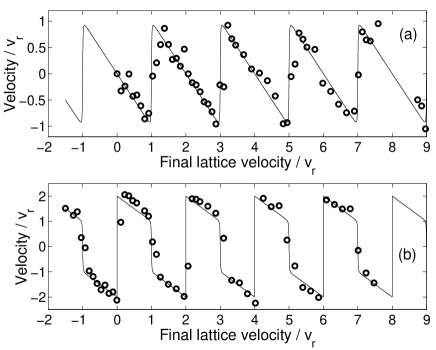
Figure 6: Same experiment as in figure 4 and fig. 5. Velocity of the atoms in the lattice frame after acceleration of the lattice, for different final lattice velocities. The velocities are deduced from fig. 4b and 5b by subtracting the velocity of the lattice. In fig. 6a the atoms are prepared in the ground state band, whereas they are prepared in the first band for the results of fig. 6b. The plain lines are the theoretical group velocity calculated for a 0.1$E_{\rm r}$ deep lattice.

V Acceleration of atoms with a broad quasimomentum distribution

In a last set of experiments, we investigate the behavior of the atoms under acceleration of the lattice when the atoms do not occupy a single quasimomentum, but rather have a wide spread of quasimomenta.

In order to prepare a broad distribution of quasimomenta, we first reproduce the experiment of Greiner2001 : while the magnetic trap is still on at a relatively high mean oscillation frequency of 100 Hz in order to increase the interaction strength, we adiabatically turn on a 5$E_{\rm r}$ deep lattice in 300 $\mu\mathrm{s}$. We then suddenly turn off the magnetic trap and let the atoms sit in the lattice for a duration ranging from 100 $\mu$s to 12 ms. We follow the evolution of the quasimomentum distribution of the atoms in the lattice by adiabatically turning off the lattice (in 300 $\mu$s) and taking an absorption image of the cloud after a 3 ms time of flight. The results are shown in fig. 7: 7a shows an image of the undisturbed condensate after the time of flight, as well as the density profile along the lattice direction, integrated along the perpendicular direction, with no lattice having been applied; in 7b, the lattice has been switched off suddenly, immediately after adiabatic loading of the lattice . The momentum components at $\pm 2\mbox{$\hbar k$}$ appear and provide a calibration of the scale; in the two last pictures, 7c and  7d, the condensate sits for respectively $t=0.5$ ms and $t=9$ ms in the lattice after which the lattice is ramped down in 300 $\mu\mathrm{s}$. After 9 ms of evolving time, when ramping down the lattice, the momentum distribution of the cloud looks essentially like a convolution of the profile of figure 7a with an almost uniformly populated momentum distribution with a $2\mbox{$\hbar k$}$ width. This corresponds to an almost completely filled first Brillouin zone.

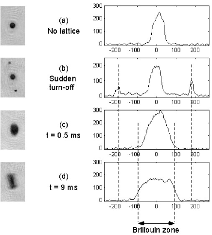
Figure 7: Dephasing of a condensate sitting in a 5$E_{\rm r}$ deep lattice for a time $t$. The time of flight has the same 3 ms duration for all the images. The right column shows the density profiles of the images in the left column, integrated perpendicular to the axis of the lattice. In fig.7a, no lattice was applied. In fig.7b the lattice was suddenly switched off. In 7c and 7d the cloud stays in the lattice for 0.5 and 9 ms respectively.

More quantitatively, from the integrated profiles we calculate the rms width of the momentum distribution of the atoms in the lab frame, after ramping down the lattice (see figure 8). Since the observed distributions result from convolution of the quasimomentum distribution with the distribution represented by fig.7a, we could in principle deconvolve them in order to get only the contribution of the quasimomentum. Instead, as a reference, we show in fig. 8 the expected rms width, convolving the experimental distribution of fig. 7a with a quasimomentum distribution filling the first Brillouin zone.

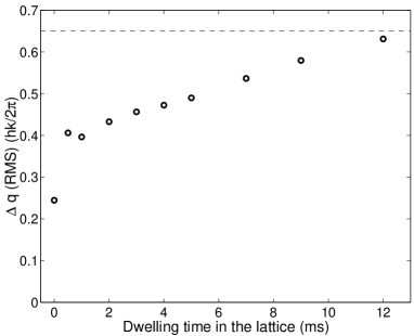
Figure 8: Evolution of the rms value of the observed the quasimomentum distribution of the atoms as a function of the time spent by the atoms in the lattice. The dotted line represents the expected width when we convolve the distribution of fig. 7a with a uniformly populated first Brillouin zone.

An explanation for this broadening comes from the mean field inhomogeneity across the cloud. In the magnetic trap, the chemical potential is independent of the position. When the lattice is super-imposed onto the magnetic trap, this is roughly still the case, provided that the lattice is not too deep. When the magnetic trap is suddenly turned off, the magnetic energy no longer compensates for the mean field energy and the chemical potential varies quadratically along the direction of the lattice. The rate of change of the phase difference between two neighboring sites then varies linearly along the lattice direction. This inhomogeneity of the density across the condensate results in a different phase evolution at each lattice site and consequently in an effective dephasing of the single particle wave-function. Remembering that the quasimomentum characterizes the phase difference from one site to another, the apparent randomization of this phase leads to a broadening of the quasimomentum distribution. Roughly speaking, when the phase difference between adjacent sites at the edge of the condensate reaches $2\pi$, the wave function of an atom looks dephased, meaning that it is a superposition of all quasimomenta in the first Brillouin zone. This phase difference between neighboring sites at the edge of the condensate being on the order of $\mu\,t/(N\hbar)$ (where $2N+1$ is the total number of sites), after a time evolution of duration $t$, the time scale for dephasing is $\sim N\,h/\mu$. Numerically, the condensate had a chemical potential $\mu/h=5$ kHz. The estimated dephasing time (the time to create a $2\pi$ phase difference between adjacent wells) is then 8 ms, which is approximately equal to the observed time to fill the Brillouin zone. This treatment neglects tunnelling between lattice sites, which would tend to equalize the phases. However, we calculate a tunnelling rate of $2\pi\times 1.5$ kHz for a 5$E_{\rm r}$ deep lattice, that is, the well-to-well tunnelling rate is faster than the differential well-to-well phase evolution. Therefore, our simple picture of dephasing is questionable, although it seems to give a reasonable description of the experiment. We believe this point deserves further study.(A more detailed study of some aspects of mean-field dephasing in a lattice has been performed in Morsch03 .)

As an additional, albeit equivalent, demonstration for the randomization of the phase, we look for diffraction after letting the condensate sit for a period of time. When we suddenly turn off the lattice, we do not observe resolved diffraction peaks when the atoms have spent more than 2 ms in the lattice. We conclude that even though we may not have uniformly filled the Brillouin zone after 2 ms, we broaden the quasimomentum distribution sufficiently that diffraction is not evident. We note that in reference Hadzibabic04 , the authors saw a diffraction pattern from an array of about 30 independent condensates. The difference is in their smaller number of lattice sites, and may also be influenced by differences in experimental details such as the optical resolution for observing the diffraction pattern, the number of diffraction peaks, and the fact that the diffraction of ref. Hadzibabic04 appears not to be observed in the “far field” . We apply the theory of Hadzibabic04 to our about 80 interfering condensates (assuming they are indeed independent which is only partially valid in our case) and found no diffraction pattern, in agreement with our observations.

We finally turn to the behavior of the dephased cloud under acceleration. After letting the cloud sit in a 5$E_{\rm r}$ deep lattice for 5 ms, more than a sufficient time to broaden the quasimomentum distribution enough that the diffraction is unresolved, we accelerate the lattice in 500 $\mu$s to a chosen final velocity. After this acceleration period, we ramp down the lattice depth to zero in 100 $\mu$s and allow for a 3 ms time of flight, as described earlier in the paper. The results are presented in fig. 9. In this figure, the mean momentum of the cloud after ramping down the lattice intensity shows no sign of the plateaus seen in fig. 4. This mean momentum is proportional to the lattice velocity, in contrast to the behavior described in section IV. In fact the atoms are dragged at the velocity of the lattice, which means that in the frame of the lattice their motion is frozen.

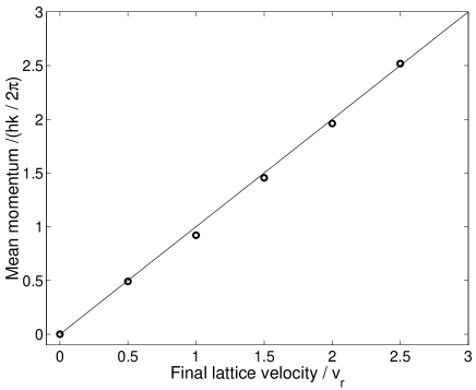
Figure 9: Acceleration of a cloud of incoherent atoms in a 5$E_{\rm r}$ deep lattice. The circles represent the momentum of the center of mass of the cloud, in the lab frame, after acceleration of the lattice. The adiabatic ramp down is followed by a 3 ms time of flight. The line represents the velocity of the lattice.

We reconcile this more intuitive behavior with the odd behavior of section IV by assuming that the first Brillouin zone is completely filled, and considering a small component of the quasimomentum distribution, centered around $q_{0}$. Upon acceleration, this population does undergo Bragg diffraction when the velocity of the lattice reaches $q_{0}+\hbar k$, and exhibits the same step behavior as the one seen in figure 4, the only difference being that the horizontal axis is shifted by $q_{0}$. All the other quasimomentum components are also Bragg reflected but at different velocities of the lattice. When one averages the different “staircase” patterns like the one shown in fig. 4 for all the quasimomenta in the first Brillouin zone, the average velocity in the lab frame is the velocity of the lattice. Another way to understand this is to calculate the average group velocity for a uniformly populated first Brillouin zone. That velocity is proportional to the average of the slope of the $E_{0}(q)$. As the band is symmetric with respect to $q=0$, this average velocity with respect to the lattice is zero and there is no motion of the center of mass of the cloud with respect to the lattice.

We now compare our above results with two recent experiments looking at thermal bosons and degenerate fermions in an optical lattice Cataliotti01 ; Modugno03 . In Cataliotti01 , a condensate surrounded by its thermal cloud is created in a several $E_{\rm r}$-deep lattice and a magnetic trap. The center of the magnetic trap is then shifted and the subsequent behavior of the two components is monitored. The authors observed that whereas the thermal component is pinned and does not oscillate in the magnetic trap, the condensate does oscillate with an oscillation frequency modified by the effective mass of the atoms in the lattice. The authors proposed an explanation based on the superfluidity of the condensate that allows it to move through the corrugated potential created by the lattice, whereas the thermal cloud does not move due to its non-superfluid nature. In light of the experiment we described above in this section, we propose an alternate explanation for those results, based only on single-particle band structure theory. In the experiment of Cataliotti01 , the condensate is prepared directly in the lattice, and occupies the Bloch state $|n=0,q=0\rangle$. Let us now assume that the thermal component has a temperature that corresponds to an energy between the ground state band and the first band of the lattice. The ground band is then almost uniformly populated, meaning that the single-particle wave-function of the atoms effectively contains all quasimomenta in the first Brillouin zone. Shifting the position of the magnetic trap is equivalent to accelerating both the lattice and the trap with respect to the lab and therefore equivalent to applying a uniform force to the atoms. As described above, the thermal cloud filling the Brillouin zone does not move with respect to the lattice (figure 9). This is what the authors of reference Cataliotti01 observed and it is completely consistent with a single-particle description, without any reference to superfluidity or critical velocity, phenomena dependent on interactions.

We finally discuss briefly the recent experiment dealing with degenerate fermions in a one-dimensional optical lattice Modugno03 ; Roati04 . In reference Modugno03 , a Fermi sea of ${}^{40}\rm{K}$ is produced in an optical lattice. The authors observe the absence of peaks in the diffraction pattern after sudden turn off of the lattice. This implies that the Fermi momentum is comparable to or larger than $\hbar k$ so that the quasimomentum extends throughout the Brillouin zone, similar to our dephased cloud of Bosons. In the same work the authors repeat, with the Fermi gas, the experiment of reference Cataliotti01 where they shift the magnetic trap with respect to the lattice. Consistent with our single-particle interpretation of the experiment (and with the single particle interpretation given in Modugno03 ), they do not observe oscillation of the Fermi cloud in the magnetic trap. In Roati04 , the authors again produce the Fermi sea in a lattice but this time they only partially fill the first Brillouin zone. As a result they do observe a diffraction pattern consisting of resolved peaks when suddenly releasing the atoms from the lattice. They also observe Bloch oscillations in their vertical lattice, due to gravity, as should be the case for a partially filled Brillouin zone. As ultra-cold indistinguishable fermions are essentially non-interacting (no $s$-wave collisions), the experiments of Modugno03 ; Roati04 illustrate single particle, i.e. non-interacting particle, behavior of a cloud of cold atoms in a lattice, as those authors point out. Collisions imply a coupling between quasimomentum states and thus the failure of the single particle (Bloch theory) description. The behavior of ultra-cold fermions is identical to our experiment and the experiment of Cataliotti01 with interacting bosons, when the influence of interactions is negligible on the time scale of the experiment. It is particularly striking that Fermions and Bosons can behave exactly in the same way under some circumstances: all that matters is the way the Brillouin zone is filled, although the way this filling occurs may depend on the quantum statistics.

VI Conclusion

In summary, we have presented a series of experiments in which a condensate is adiabatically loaded into an optical lattice, preparing the atoms in a single Bloch state. In a first set of experiments, the lattice is initially moving, and the atoms come back to rest in the lab frame after the adiabatic turn off of the lattice, leading to non-intuitive behavior for this “quantum conveyor belt”. In a second set of experiments, we act on the prepared quasimomentum distribution by accelerating the lattice. We then analyze the new quasimomentum distribution by again adiabatically ramping down the lattice, and again observed non-intuitive behavior. We observe discrete jumps in the resulting momentum distribution, depending upon the velocity of the lattice. These jumps are reminiscent of Bragg diffraction at each avoiding crossing due to the laser coupling and are equivalent to Bloch oscillations. In a last set of experiments, we let the initial quasimomentum distribution evolve under the influence of interactions between the atoms, leading to the filling of the first Brillouin zone. The resulting cloud now exhibits a different behavior under acceleration of the lattice, i.e. the cloud appears to be frozen in the frame of the lattice. Finally we showed the similarities between the behavior of a cold thermal cloud and that of a cloud of degenerate fermions in an accelerated optical lattice, when the quasimomentum extends throughout the first Brillouin zone.

Among the issues that we believe deserve further studies, both experimentally and theoretically, is the competition between phase winding and tunnelling, that is to say how atoms lose their well-to-well phase coherence. Furthermore, we considered in this paper the dephasing of the wave-function due to the density profile of the cloud, but the quantum fluctuation of the atom number in each well is also a source of effective decoherence that should be explored. We also emphasize that the time scales of our experiments are very short with respect to other experiments, such as the one described in Morsch03 ; Cataliotti01 .

Finally we note that the method of section IV could be useful for precision measurements, as described in ref. Battesti04 .

- (1) M.H. Anderson, J.R. Ensher, M.R. Matthews, C.E. Wieman, E.A. Cornell, Science 269, 198 (1995).
- (2) F. Dafolvo, S. Giorgini, L. P. Pitaevskii, and S. Stringari, Rev. Mod. Phys. 71, 463 (1999).
- (3) J. Hecker-Denschlag, J. E. Simsarian, H. Häffner, C. McKenzie, A. Browaeys, D. Cho, K. Helmerson, S. L. Rolston, and W. D. Phillips, J. Phys. B 6, 1 (2002).
- (4) L. Fallani, F.S. Cataliotti, J. Catani, C. Fort, M. Modugno, M. Zawada, and M. Inguscio, Phys. Rev. Lett. 91, 240405 (2003).
- (5) O. Morsch, J.H. Müller, M. Cristiani, D. Ciampini, and E. Arimondo, Phys. Rev. Lett. 87 140402 (2001).
- (6) B. Eiermann, P. Treutlein, T. Anker, M. Albiez, M. Taglieber, K.-P. Marzlin, and M. K. Oberthaler, Phys. Rev. Lett. 91, 060402 (2003).
- (7) M. Kozuma, L. Deng, E.W. Hagley, J. Wen, R. Lutwak, K. Helmerson, S.L. Rolston, W.D. Phillips, Phys. Rev. Lett. 82, 871 (1999).
- (8) N. Ashcroft and D. Mermin, “Solid State Physics”, Saunders College (1976).
- (9) W. Petrich, M. H. Anderson, J. R. Ensher, and E. Cornell, Phys. Rev. Lett. 74, 3352 (1995).
- (10) J. Stenger, S. Inouye, A.P. Chikkatur, D.M. Stamper-Kurn, D.E. Pritchard, and W. Ketterle, Phys. Rev. Lett. 82, 4569 (1999).
- (11) A. Kastberg, W. D. Phillips, S. L. Rolston, and R. J. C. Spreeuw, Phys. Rev. Lett. 74, 1542 (1995).
- (12) M. Greiner, I. Bloch, O. Mandel, T. W. Hänsch, T. Esslinger, Phys. Rev. Lett. 87, 160401 (2001).
- (13) M. Ben Dahan et al., Phys. Rev. Lett. 76, 4508 (1996), S. R. Wilkinson et al., Phys. Rev. Lett. 76, 4512 (1996).
- (14) O. Morsch, J. H. Müller, M. Cristiani, P. B. Blakie, C. J. Williams, P. S. Julienne, and E. Arimondo, Phys. Rev. A 67, 031603 (2003).
- (15) Z. Hadzibabic, S. Stock, B. Battelier, V. Bretin, and J. Dalibard, Phys. Rev. Lett. 93, 180403 (2004).
- (16) F.S. Cataliotti, S. Burger, C. Fort, P. Maddaloni, F. Minardi, A. Trombettoni, A. Smerzi, M. Inguscio, Science 293, 843 (2001); S. Burger, F. S. Cataliotti, C. Fort, F. Minardi, and M. Inguscio, M. L. Chiofalo and M. P. Tosi, Phys. Rev. Lett. 86, 4447 (2001).
- (17) G. Modugno, F. Ferlaino, R. Heidemann, G. Roati, and M. Inguscio, Phys. Rev. A 68, 011601 (2003).
- (18) G. Roati, E. de Mirandes, F. Ferlaino, H. Ott, G. Modugno, and M. Inguscio, Phys. Rev. Lett. 92, 230402 (2004).
- (19) R. Battesti, P. Clad , S. Guellati-Kh lifa, C. Schwob, B. Gr maud, F. Nez, L. Julien, and F. Biraben, Phys. Rev. Lett. 92, 230402 (2004).