Perturbation of magnetostatic modes observed by FMRFM

Abstract

Magnetostatic modes of Yttrium Iron Garnet (YIG) films are investigated by ferromagnetic resonance force microscopy (FMRFM). A thin film “probe” magnet at the tip of a compliant cantilever introduces a local inhomogeneity in the internal field of the YIG sample. This influences the shape of the sample’s magnetostatic modes, thereby measurably perturbing the strength of the force coupled to the cantilever. We present a theoretical model that explains these observations; it shows that tip-induced variation of the internal field creates either a local “potential barrier” or “potential well” for the magnetostatic waves. The data and model together indicate that local magnetic imaging of ferromagnets is possible, even in the presence of long-range spin coupling, through the induction of localized magnetostatic modes predicted to arise from sufficiently strong tip fields.

In the past decade, the possibility of using magnetic degrees of freedom in electronic devices has attracted the attention of the semiconductor industry. There are numerous proposals to incorporate spin degrees of freedom into electronics creating spin-electronic or spintronic devices Heinrich (2000). These devices require a thorough understanding of the magnetization dynamics on the submicron scale. Magnetic resonance force microscopy (MRFM) has proven itself to be a three dimensional nondestructive imaging technique that can be applied to electron Rugar et al. (1992); Hammel et al. (1995); Rugar et al. (2004) and nuclear Rugar et al. (1994) resonance experiments. In MRFM a micromagnet (tip magnet) is placed on a compliant cantilever. The time variation of the amplitude of the precessing spins will produce a force on the cantilever via the gradient field of the tip magnet. In addition the tip magnet produces a perturbation in the magnetic field in the sample producing a small bowl shaped region in which the spins are at resonance, the resonance slice. This resonance slice can be highly localized (on the order of the size of the tip magnet) thus allowing subsurface detection of spins with submicron resolution. A recent experiment reported the detection of a single spin in resonance Rugar et al. (2004).

Ferromagnetic Resonance Force Microscopy (FMRFM) Zhang et al. (1996); Loehndorf et al. (2000); Charbois et al. (2002) is a variation of MRFM that enables the three dimensional, high sensitivity and high resolution qualities of MRFM to be applied in the characterization of the dynamic magnetic properties of ferromagnetic thin films and multilayers at the micron scale. The tip field penetrates magnetic and nonmagnetic materials allowing one to investigate buried structures and interfaces. Recent publications have shown the ability of FMRFM to determine the nature and magnitude of terms contributing to the internal field Loehndorf et al. (2000), dispersion relations of magnetostatic modes Zhang et al. (1996); Charbois et al. (2002); Midzor et al. (2000) and relaxation processes in micron size samples Klein et al. (2003). Ferromagnetically coupled systems pose unique challenges for magnetic resonance imaging due to the strong coupling between the spins. The resulting magnetostatic/exchange resonance modes involve spins occupying the entire sample not just those within the resonance slice Midzor et al. (2000). Therefore, local imaging capability of MRFM is lost in the case of ferromagnetic samples.

In this Letter we report the first direct observation of the variation of the magnetostatic mode amplitudes due to the local perturbation of the internal field. The localized field is produced by the sharp magnetic tip when it is scanned across the surface of Yttrium Iron Garnet (YIG) samples. The experimental results are in excellent agreement with theoretical predictions. In addition, based on our theoretical model, we propose that it is possible to generate a highly localized mode and recover, in part, the advantages of local imaging capabilities of MRFM. These localized magnetic modes will provide an exciting opportunity to investigate static and dynamic magnetic properties of micron-size defects (imperfections) embedded in ferromagnetic samples without the interference of edge effects.

The experiments were performed using an ambient FMRFM system in the perpendicular geometry Midzor et al. (2000). The sample is attached to a microstrip resonator having a resonance frequency of 7.4 GHz. The silicon cantilever’s resonance frequency, the spring constants, and the ambient Q-factor are 17.8 kHz, 0.4 N/m, and 90, respectively. The cantilever displacement is monitored by 850 nm fiber optic interferometer. The cantilever tip was coated with a 250 nm CoPt film ($M_{s}=800$ emu/cm³) and annealed in an external magnetic field of 80 kOe oriented along the tip axis of the cantilever. This resulted in a coercive field of 10 kOe Signoretti et al. (2004). The magnetic tip generates a localized tip field, $h_{\rm tip}$, which can be aligned either parallel ($h_{\rm tip}>0$) or antiparallel ($h_{\rm tip}<0$) to the external dc field, $H_{\rm ext}$. Based on a model of the magnetic tip, the strength of the tip field and the tip field gradient at the tip-sample separation $z=1$ $\mu$m were estimated to be 80 G and 50 G/$\mu$m for $h_{\rm tip}>0$.

In the following section we present experimental data that confirm the importance of local probe-induced phenomena. Typical measured spectra obtained on the $20\times 80$ $\mu$m² YIG sample are shown in Fig. 1. The magnetostatic modes are labelled by $(n_{x},n_{y})$, where $n_{x}$ and $n_{y}$ represent the number of half wavelengths along the sample width and length, respectively. In the presence of a uniform bias field and a homogeneous driving rf field only modes with odd values of $n_{x}$ and $n_{y}$ have a net dipole moment that will couple to the rf field Wigen et al. (to be published). However, if the symmetry of the magnetic field is broken by the presence of the localized tip field, the magnetostatic modes having $n_{x}$ and/or $n_{y}$ even can have a net dipole moment and be excited. We now discuss the cases of parallel and antiparallel tip orientations.

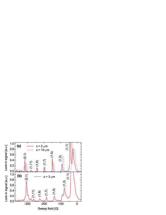
Figure 1: Typical FMRFM spectra measured in the center ($y=0$ $\mu$m) of the $20\times 80\,\mu$m² sample for (a) $h_{\rm tip}>0$ and (b) $h_{\rm tip}<0$, respectively. The dashed and the solid lines correspond to the tip-sample separation of 10 $\mu$m and 2 $\mu$m, respectively. Zero sweep field corresponds to the resonance field of the homogeneous mode $\omega/\gamma+4\pi M_{s}=4.4$ kG.

$h_{\rm tip}>0$: To investigate the effects of this perturbation quantitatively, we first discuss the case when the magnetic field of the tip magnet adds to the bias magnetic field. For a weak tip field ($h_{\rm tip}\approx 0$) applied at the center of the sample the mode amplitudes are observed to decrease monotonically with increasing $n_{x}$ and $n_{y}$. Such a spectrum is shown by the dashed line in Fig. 1a for $z=10$ $\mu$m. At that distance the magnetic field generated by the tip magnet is on the order of 2 G. As the tip approaches the sample surface, the magnetic tip field increases. This results in a dramatic change of the measured spectra as illustrated by the solid line in Fig. 1a. There are two main features to be noted: (i) the spectrum is shifted to a lower resonance field by $(8\pm 1)$ G and (ii) the amplitude of modes (1,5) and (1,9) are enhanced relative to modes (1,3), (1,7), and (1,11). The resonance field shift is due to the spatially-averaged tip field which adds to the external field. Notice, that the principal mode ($n_{x}=n_{y}=1$) is also split. We attribute the mode on the high field side to be a localized surface mode Wigen (1984).

To demonstrate the subtle details of the effect of the increasing tip field, the force intensity for modes (1,3) and (1,5) is plotted in Fig. 2 as a function of the tip-sample separation. As the tip field gradient increases with decreasing distance the FMRFM signal increases. However, the intensity of the (1,3) mode decreases dramatically for $z<3$ $\mu$m and at $z=2.5$ $\mu$m its intensity becomes even lower than the intensity of the (1,5) mode. For $z<2$ $\mu$m the intensity of the (1,5) mode decreases as well. These effects can be explained by the model proposed below, see Fig. 2b.

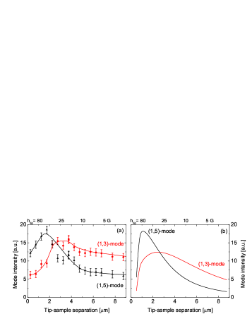
Figure 2: (a) The mode intensity of the (1,3) and (1,5) mode as a function of the tip-sample separation. The tip was placed above the middle of the $20\times 80$ $\mu$m² sample. The solid lines are a spline fit to data to guide the eye. (b) The theoretical prediction using a cylindrical magnetic tip.

	I(1,3)/I(1,5)	I(1,5)/I(1,7)	I(1,7)/I(1,9)
$h_{\rm tip}>0$	$0.6\pm 0.1$	$2.9\pm 0.1$	$1.0\pm 0.2$
$h_{\rm tip}\approx 0$	$1.6\pm 0.1$	$1.9\pm 0.1$	$1.5\pm 0.2$
$h_{\rm tip}<0$	$2.4\pm 0.2$	$1.1\pm 0.3$	$1.9\pm 0.4$

Table 1: The intensity ratios for modes (1,3), (1,5), (1,7), and (1,9) in the presence of a strong positive tip field ($h_{\rm tip}>0$), a weak tip field ($h_{\rm tip}\approx 0$), and a negative tip field ($h_{\rm tip}<0$). Corresponding spectra are plotted in Fig. 1.

$h_{\rm tip}<0$: By reversing the orientation of the applied magnetic field without reversing $h_{\rm tip}$, the magnetic field of the tip subtracts from the homogeneous bias field. For a tip-sample separation below 2 $\mu$m, the modes (1,3), (1,7), and (1,11) are now stronger compared to modes (1,5) and (1,9), see Fig. 1b. This is exactly opposite to what is observed for $h_{\rm tip}>0$. Table 1 summarizes the intensity ratios of the subsequent resonant modes when the tip field is weak and the magnetostatic modes are practically unperturbed, $h_{\rm tip}\approx 0$ line and for strong tip fields, $h_{\rm tip}>0$ and $h_{\rm tip}<0$. There are two notable features: (i) the values in the first row are lower/higher/lower than values for $h_{\rm tip}\approx 0$ while the values in the third row are higher/lower/higher than the values for $h_{\rm tip}\approx 0$. This reinforces the conclusions made earlier that for $h_{\rm tip}>0$, the modes (1,5) and (1,9) are enhanced, while for $h_{\rm tip}<0$ the modes (1,3) and (1,7) are enhanced. (ii) The first and third columns are ascending while the second column is descending.

The influence of the perturbation field of the probe magnet is further demonstrated in lateral scans taken along the long axis of the sample at $z\approx 3$ $\mu$m. Fig. 3a shows the experimental data of the force amplitudes for the ($1,n_{y}$) modes as a function of position. Three interesting features are observed: (i) As the tip is moved from the center of the sample, the field of the tip magnet has broken the even symmetry of the internal field. As a result the “hidden” (1,2) mode is excited. (ii) For the (1,3) mode, the intensity at $y=0$ $\mu$m is strongly suppressed while at the position of the next maxima in the magnetostatic mode at $y=\pm 26$ $\mu$m the intensity is enhanced. (iii) Mode (1,5) shows very little variation as a function of position of the tip. Therefore, the lateral resolution can be estimated to be approximately 20 $\mu$m. This is in good agreement with the theoretical predictions (Fig. 3b).

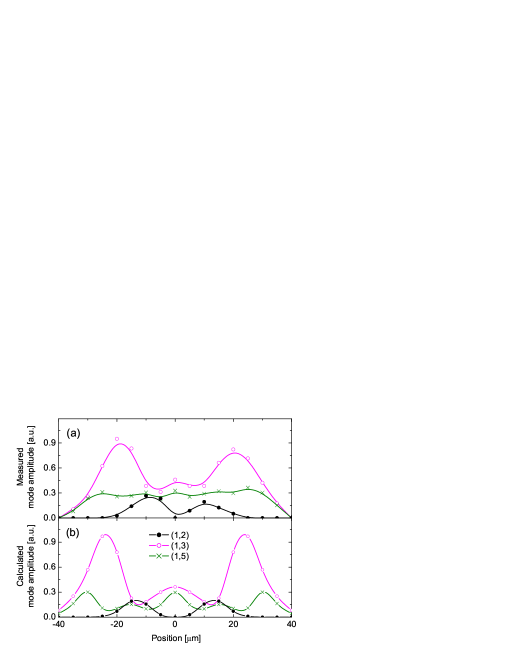
Figure 3: The mode intensity for the (1,2), (1,3), and (1,5) modes as the tip is scanned along the long axis of the $20\times 80\,\mu$m² sample. The external dc field and the probe field are parallel. The tip-sample separation $z\approx 3$ $\mu$m. (a) Measured response. (b) Calculated amplitude.

These unusual characteristics are understood within a theoretical model which is based on a linearized Landau-Lifshitz-Gilbert (LLG) equation of motion that include a spatially dependent tip field and Maxwell’s equations. The external dc field is parallel to the sample normal and the driving rf field, $h_{\rm rf}$, lies in the plane of the sample and is considered to be homogeneous over the entire sample. The cantilever tip field, $h_{\rm tip}({\mbox{\boldmath$r$}})$, is considered to be either parallel, $h_{\rm tip}>0$, or antiparallel, $h_{\rm tip}<0$, to the external field ${\mbox{\boldmath$H$}}_{\rm ext}$.

The linearized LLG equation of motion and Maxwell’s equations neglecting displacement currents can be written as (in cgs units)

$$\frac{\partial{\mbox{\boldmath$M$}}}{\partial t}=-\gamma\left[{\mbox{\boldmath$M$}}\times{\mbox{\boldmath$H$}}_{\rm eff}\right]+\frac{\alpha}{M_{s}}\left[{\mbox{\boldmath$M$}}\times\frac{\partial{\mbox{\boldmath$M$}}}{\partial t}\right]\;,$$ (1)

$$\nabla\times{\mbox{\boldmath$H$}}=0\;,\qquad\nabla\cdot({\mbox{\boldmath$H$}}+4\pi{\mbox{\boldmath$M$}})=0\,,$$ (2)

where $\gamma$ ($=1.84\times 10^{7}$ Oe^-1s^-1) is the absolute value of gyromagnetic ratio, $M_{s}$ ($=140$ erg/cm³) is the saturation magnetization, and $\alpha$ ($=0.0045$) is the dimensionless Gilbert damping parameter. The internal effective field, ${\mbox{\boldmath$H$}}_{\rm eff}$, is given by

$${\mbox{\boldmath$H$}}_{\rm eff}=\left(h_{x}+h_{\rm rf},h_{y},H_{\rm ext}-4\pi M_{s}+h_{\rm tip}\left({\mbox{\boldmath$r$}}\right)\right)\,.$$ (3)

Eq. (1) is solved in a small angle approximation; $|{\mbox{\boldmath$m$}}|\ll M_{s}$, where $m$ represents the transverse rf component of the magnetization vector. The boundary conditions are assumed to be

$${\mbox{\boldmath$m$}}|_{x=\pm L_{x}/2}={\mbox{\boldmath$m$}}|_{y=\pm L_{y}/2}=0\,.$$ (4)

The unique feature in the model is treating the tip field as a non-local perturbation and determining its effect on the magnetostatic modes. Using Eq. 2, the rf magnetic field $h$ is expressed in terms of the magnetization ${\mbox{\boldmath$m$}}({\mbox{\boldmath$r$}})$ as a linear functional ${\mbox{\boldmath$h$}}[{\mbox{\boldmath$m$}}({\mbox{\boldmath$r$}})]$ resulting in the non-local relationship

$$\hat{K}{\mbox{\boldmath$m$}}({\mbox{\boldmath$r$}})+h_{0}({\mbox{\boldmath$r$}}){\mbox{\boldmath$m$}}({\mbox{\boldmath$r$}})=\Delta\Omega{\mbox{\boldmath$m$}}({\mbox{\boldmath$r$}})+h_{\rm rf}\,,$$ (5)

$$\Delta\Omega=\frac{1}{4\pi M_{s}}\left(\frac{\omega}{\gamma}-H_{\rm ext}+4\pi M_{s}\right)\,,$$ (6)

$$h_{0}({\mbox{\boldmath$r$}})=\frac{h_{\rm tip}({\mbox{\boldmath$r$}})}{4\pi M_{s}}\,.$$ (7)

The operator $\hat{K}$ represents a linear integral transformation defined by

$$\hat{K}f_{{\mbox{\boldmath$k$}}}({\mbox{\boldmath$r$}})=\omega_{{\mbox{\boldmath$k$}}}f_{{\mbox{\boldmath$k$}}}({\mbox{\boldmath$r$}})\,,$$ (8)

where $f_{{\mbox{\boldmath$k$}}}$ represents the unperturbed magnetostatic modes given by

$$f_{{\mbox{\boldmath$k$}}}(x,y)=\sin{\left\{k_{x}\left(x+L_{x}/2\right)\right\}}\,\sin{\left\{k_{y}\left(y+L_{y}/2\right)\right\}}$$ (9)

and $\omega_{{\mbox{\boldmath$k$}}}$ is their dispersion relation given by the Damon-Eshbach theory Eshbach and Damon (1960). The wave-vectors $k$ are chosen to satisfy the “pinned” boundary conditions, Eq. 4. The new basis of the magnetostatic modes ${m}_{n}({\mbox{\boldmath$r$}})$ can be found by solving the homogeneous equations

$$\left[\hat{K}+h_{0}({\mbox{\boldmath$r$}})\right]m_{n}({\mbox{\boldmath$r$}})=\Delta\Omega_{n}m_{n}({\mbox{\boldmath$r$}})\,.$$ (10)

The FMRFM signal is proportional to the force acting on the cantilever which can be written as

$$F_{\rm FMRFM}\approx d\int_{A}M_{z}({\mbox{\boldmath$r$}})\cdot\nabla_{z}h_{\rm tip}({\mbox{\boldmath$r$}})\,{\rm d}x{\rm d}y\,,$$ (11)

where $M_{z}({\mbox{\boldmath$r$}})=M_{s}-|{\mbox{\boldmath$m$}}|^{2}/2M_{s}$ is the longitudinal component of magnetization, $d$ is the thickness of the film and $A$ represents the area of the sample. A detailed discussion of the theory will be presented elsewhere Putilin et al. (to be published).

Eq. 10 offers an interesting interpretation; It is similar to the time-independent Schrödinger equation with the kinetic energy-like term given by $\omega_{{\mbox{\boldmath$k$}}}$ in Eq. 8. The normalized tip field $h_{0}({\mbox{\boldmath$r$}})$ in Eq. 7 plays the role of a potential energy. When the tip field is parallel to the external field, $h_{0}({\mbox{\boldmath$r$}})>0$, it creates a potential barrier for the magnetostatic modes, while $h_{0}({\mbox{\boldmath$r$}})<0$ yields a potential well.

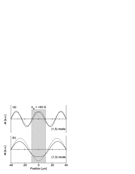
Figure 4: The calculated magnetostatic modes of the $20\times 80$ $\mu$m² sample with the tip located at the center of the film. The unperturbed (dashed) and perturbed (solid) modes are plotted for a potential barrier $h_{\rm tip}=+60$ G. Notice, that the wavelength of the mode is increased in the perturbed region (shaded). (a) For the (1,5) mode this region increases the net dipole moment and therefore increases the FMRFM signal. (b) For (1,3) mode this region decreases the net dipole moment and therefore reduces the FMRFM signal.

This analogy provides qualitative insight into how the magnetostatic modes are modified by the tip magnetic field.

$h_{\rm tip}>0$: The effect of the perturbation field when the tip field is parallel to the bias field is to increase the wavelength of the magnetostatic mode in the region near the tip. Fig. 4 shows this effect when the tip is located at the center of the film. If $m$ is positive (i.e., when $m$ is parallel to the net dipole moment of the mode) in the region near the tip as in the case of mode (1,5) shown in Fig. 4a, the net dipole moment of the mode will be increased and therefore the FMRFM signal is enhanced. On the other hand, if $m$ is negative (i.e., when $m$ is antiparallel to the net dipole moment of the mode) in the region of the tip field as shown for mode (1,3) in Fig. 4b, the net dipole moment will be decreased and therefore the FMRFM signal for that mode is suppressed.

As the tip approaches the surface of the sample the tip field gradient increases and therefore the FMRFM signal increases, see Fig. 2. However, when the field separation of the magnetostatic mode $4\pi M_{s}\Delta\Omega$ (see Eq. 6) is smaller than the tip field $h_{\rm tip}$, the mode becomes evanescent. This decreases the amplitude of the magnetostatic wave in the vicinity of the tip magnet resulting in a reduced FMRFM signal even though the gradient of the field is increased. This is demonstrated in Fig. 2b.

When the tip magnet is scanned across the sample, the transverse component of the magnetization $m$ changes sign at the next lobe position; At $y=0$ $\mu$m, the transverse component of $m$ for the (1,3) mode is negative and therefore the intensity of this mode is strongly suppressed. On the other hand, at $y=\pm 26$ $\mu$m, $m$ is positive and, as observed in Fig. 4 this mode is strongly enhanced.

$h_{\rm tip}<0$: In the case of the potential well the results are exactly the opposite to those for a potential barrier ($h_{\rm tip}>0$). If $m$ is negative in the region of the tip magnet as is the case for mode (1,3), the wavelength of the wave in the region of the perturbing tip field is decreased and the coupling of the mode to the rf field is increased. Consequently the FMRFM intensity of the mode is enhanced. On the other hand, if $m$ is positive in the region of the tip field as for mode (1,5), the net dipole moment will be decreased and therefore the FMRFM signal for that mode is suppressed.

Extending the Schrödinger equation analogy to the case of a deep narrow potential well, a highly localized magnetic mode can be excited Putilin et al. (to be published). The properties of this localized mode would be independent of the sample size and therefore of any edge imperfections that might be introduced in the sample preparation. Scanning the local mode about the sample would allow one to extract variations in the local magnetic properties of the ferromagnetic samples. This makes FMRFM a unique experimental method allowing the investigation of local magnetic properties of the ferromagnetic samples independent on the sample dimensions, shape and/or defects at the sample edge. Incorporation of advanced nanomagnetic probe tips should enable next-generation FMRFM systems capable of imaging local magnetic properties with sub-micron lateral resolution.

In conclusion, it has been demonstrated that the magnetic field of the tip magnet introduces a local inhomogeneity in the internal field of a $20\times 80\,\mu$m² YIG film. This influences the shape of the samples magnetostatic modes, thereby measurably perturbing the strength of the force coupling to the cantilever. Using a hard magnetic coating on the tip, we are able to investigate the magnetostatic modes when the tip field is parallel ($h_{\rm tip}>0$) and antiparallel ($h_{\rm tip}<0$) to the external dc field. The condition $h_{\rm tip}>0$ can be visualized as a potential barrier in the Schrödinger-like equation analogy, and modes (1,5) and (1,9) are enhanced while modes (1,3) and (1,7) were suppressed. In contrast with this is the case for $h_{\rm tip}<0$ corresponding to a potential well in the Schrödinger-like equation analogy. Here the observed effect is exactly the opposite to the case for $h_{\rm tip}>0$. These results are in excellent agreement with the proposed theory indicating, that an inhomogeneity in the internal field can also be successfully included into FMRFM experiments. Furthermore, highly localized magnetostatic modes are predicted which are suitable for local imaging of ferromagnetic samples.

We thank to Melissa M. Midzor for assistance and discussions. We gratefully acknowledge financial support from ONR MURI under grant DAAD 19-01-0541. P.E.W. was supported by R.J. Yeh fund during the course of this research.

References

- Heinrich (2000) B. Heinrich, Canadian Journal of Physics 78, 161 (2000).
- Rugar et al. (1992) D. Rugar, C. Yannoni, and J. Sidles, Nature 360, 563 (1992).
- Hammel et al. (1995) P. C. Hammel, Z. Zhang, G. Moore, and M. L. Roukes, J. Low Temp. Phys. 271, 59 (1995).
- Rugar et al. (2004) D. Rugar, R. Budakian, H. Mamin, and B. Chui, Nature 430, 329 (2004).
- Rugar et al. (1994) D. Rugar, O. Zuger, S. Hoen, C. S. Yannoni, H.-M. Vieth, and R. Kendrick, Science 264, 1560 (1994).
- Zhang et al. (1996) Z. Zhang, P. C. Hammel, and P. E. Wigen, Appl. Phys. Lett. 68, 2005 (1996).
- Loehndorf et al. (2000) M. Loehndorf, J. Moreland, and P. Kabos, App. Phys. Lett. 76, 1176 (2000).
- Charbois et al. (2002) V. Charbois, V. Naletov, J. Youssef, and O. Klein, J. Appl. Phys. 91, 7337 (2002).
- Midzor et al. (2000) M. M. Midzor, P. E. Wigen, D. Pelekhov, W. Chen, P. C. Hammel, and M. L. Roukes, J. Appl. Phys. 87, 6493 (2000).
- Klein et al. (2003) O. Klein, V. Charbois, V. Naletov, and C. Fermon, Phys. Rev. B 67, 220407(R)/1 (2003).
- Signoretti et al. (2004) S. Signoretti, C. Beeli, and S. Liou, J Magn Magn Mater 272-76, 2167 (2004).
- Wigen et al. (to be published) P. E. Wigen, M. L. Roukes, and P. C. Hammel, Ferromagnetic resonance force microscopy (Springer-Verlag, to be published).
- Wigen (1984) P. E. Wigen, Thin Solid Films 114, 135 (1984).
- Eshbach and Damon (1960) J. Eshbach and R. Damon, Phys. Rev. 118, 1208 (1960).
- Putilin et al. (to be published) A. Putilin, M. C. Cross, and M. L. Roukes (to be published).