Effects of thermal fluctuations on the magnetic behavior of mesoscopic superconductors

Abstract

We study the influence of thermal fluctuations on the magnetic behavior of square mesoscopic superconductors. The strength of thermal fluctuations are parameterized using the Ginzburg number, which is small ($G_{i}\approx 10^{-10}$) in low-$T_{c}$ superconductors and large in high-$T_{c}$ superconductors ($G_{i}\approx 10^{-4}$). For low-$T_{c}$ mesoscopic superconductors we found that the meta-stable states due to the surface barrier have a large half-life time, which leads to the hysteresis in the magnetization curves as observed experimentally. A very different behavior appears for high-$T_{c}$ mesoscopic superconductors where thermally activated vortex entrance/exit through surface barriers is frequent. This leads to a reduction of the magnetization and a non-integer average number of flux quanta penetrating the superconductor. The magnetic field dependence of the probability for the occurrence of the different vortex states and the fluctuations in the number of vortices are studied.

I Introduction

In the last decade, the study of vortex matter in finite mesoscopic superconductors attracted a lot of attention, both experimentallyLN373m ; LPRB60v ; LN408m ; LPRL86m ; GN390 ; GN396 ; GN407 ; Lindelof ; kanda_baelus1 ; kanda_baelus2 and theoretically.PRB57v ; PRL81v ; PRL83v ; PRB59 ; PPRL84 ; PC369p ; PRB65 ; HD1 ; HD2 Most of the experimental studies on mesoscopic superconductors deal with conventional low-$T_{c}$ superconductors. Resistivity measurements are widely used to obtain information on the superconducting/normal transition. LN373m ; LPRB60v ; LN408m ; LPRL86m With ballistic Hall magnetometry it is possible to measure deep inside the superconducting phase diagram and to obtain information on the magnetization of the different superconducting states.GN390 ; GN396 ; GN407 ; Lindelof Recently, A. Kanda et al. developed the multiple-small-tunnel-junction method to distinguish between multivortex and giant vortex states in mesoscopic superconductors. kanda_baelus1 ; kanda_baelus2 Theoretically, studies of the Ginzburg-Landau free energy PRB57v ; PRL81v ; PRL83v ; PRB59 ; PPRL84 ; PC369p ; PRB65 and the time dependent Ginzburg-Landau equationsHD1 ; HD2 have shown how the magnetic and dynamics properties depend on the sample sizes and geometry. In particular the mesoscopic samples can develop Abrikosov multivortex states PRL81v and depending on the size of the sample it is possible to observe first or second order transitions.PRB57v One interesting characteristic of the magnetic properties of mesoscopic superconductors is the behavior of the dc magnetization curves. In mesoscopic superconductors there is a reinforcement of the surface barrier for entrance and exit of vortices.PRL83v ; PRB59 ; HD1 The surface barriers allow for the existence of meta-stable states of constant vorticity as a function of magnetic field and lead to a magnetization curve with discontinuous jumps, which have been observed experimentally.GN390 All these results are for conventional low-$T_{c}$ superconductors, where the effects of thermal fluctuations are generally small.

A very different situation occurs in macroscopic high-$T_{c}$ superconductors where the effects of thermal fluctuations are important. In particular, fluctuations affect the dynamics of vortex entrance through the surface barriers. burlachkov91_exp ; burlachkov94_teo ; schilling ; civale ; niderost Recently, there has been interest in the study of the magnetic properties of micron-sized high-$T_{c}$ superconductors wang ; kogan-clem . Single fluxoid transitions and two-state telegraph noise was measured in thin film rings at temperatures close to $T_{c}$.kogan-clem The fluxoid transitions were explained by thermally activated penetration of vortices.

The magnetic and dynamic behavior of mesoscopic superconductors is greatly influenced by surface barriers and geometry effects.PRL83v ; PRB59 ; PRB65 ; HD1 As a consequence, thermal fluctuations in mesoscopic high-$T_{c}$ superconductors could lead to interesting phenomena due to thermally activated vortex entrance/exit through surface barriers.

In the present paper we study the effects due to thermal fluctuations on the vortex entry in square mesoscopic superconductors. We solve numerically the time-dependent Ginzburg-Landau equations taking into account demagnetizing effects and thermal noise fluctuations. The strength of thermal noise fluctuations is parameterized by the Ginzburg number. For conventional low-$T_{c}$ superconductors the Ginzburg number is small, while for high-$T_{c}$ superconductors this parameter is large. We compare results obtained from the minimization of the mean field free energy, corresponding to the equilibrium states in the absence of thermal fluctuations, with the results from the time dependent Ginzburg Landau (TDGL) dynamics with small Ginzburg number (corresponding to conventional low-$T_{c}$ superconductors) and the results for TDGL dynamics with large Ginzburg number (corresponding to high-$T_{c}$ superconductors). The magnetization, the number of vortices, the free energy, etc are calculated in each case. We find very good agreement between the results of free energy minimization and the results of TDGL with small Ginzburg number. In the case of a large Ginzburg number the TDGL approach gives different and new results for the magnetization and the vortex dynamics.

The paper is organized as follows. In Section II we give the two theoretical formalisms used in the present paper. First we describe how we solve the TDGL equations, obtaining the magnetic fields via the Biot-Savart law and including thermal fluctuations. Secondly, we describe the solution of the stationary Ginzburg-Landau equations, when the magnetic field is solved via Ampere’s law. In Section III the results of the TDGL theory are compared with the ones of the stationary GL theory. In a first step, we neglect the thermal fluctuations and compare the results both at zero and finite temperature. In a second step, we include thermal fluctuations in our calculations and compare the results with small and large Ginzburg number. Finally, in Section IV we present our conclusions.

II Theoretical formalism

II.1 Time-dependent Ginzburg-Landau theory

We solve the time-dependent Ginzburg-Landau equations, in the gauge where the electrostatic potential is zero, and taking into account thermal fluctuations (see Ref. enomoto, ; hohenberg, ), i.e.

$$\Gamma^{-1}_{\Psi}\frac{\partial\Psi}{\partial t} = -\frac{\delta{\cal G}}{\delta\Psi^{*}}+\zeta_{\Psi}(\vec{r},t),$$ (1)

$$\Gamma^{-1}_{A}\frac{\partial\vec{A}}{\partial t} = -\frac{\delta{\cal G}}{\delta\vec{A}}+\vec{\zeta}_{A}(\vec{r},t),$$ (2)

where $\Psi$ is the order parameter and $\vec{A}$ the vector potential. $\Gamma_{\Psi}=2mD/\hbar^{2}$ and $\Gamma_{A}=c^{2}/\sigma_{n}$ are kinetic coefficients where $\sigma_{n}$ is the quasiparticle conductivity and $D$ is the electron diffusion constant. $\zeta_{\Psi}(\vec{r},t)$ and $\vec{\zeta}_{A}(\vec{r},t)$ are Langevin thermal noise with average $\langle\zeta_{\Psi}\rangle=\langle\zeta_{A}\rangle=0$ and the following correlations enomoto ; hohenberg :

$$\langle\zeta_{\Psi}^{*}(\vec{r},t)\zeta_{\Psi}(\vec{r}^{\prime},t^{\prime})\rangle=2k_{B}T\Gamma^{-1}_{\Psi}\delta(\vec{r}-\vec{r}^{\prime})\delta(t-t^{\prime}),$$ (3)

$$\langle\zeta_{A}^{i}(\vec{r},t)\zeta_{A}^{j}(\vec{r}^{\prime},t^{\prime})\rangle=2k_{B}T\Gamma^{-1}_{A}\delta(\vec{r}-\vec{r}^{\prime})\delta(t-t^{\prime})\delta_{ij}.$$ (4)

The difference $\cal{G}$ between the superconducting and the normal state Gibbs free energy is given by

$${\cal G} = {\cal G}_{s}-{\cal G}_{n}$$ (5)

$$= \int\Bigl{[}\alpha(T)|\Psi|^{2}+\frac{1}{2}\beta|\Psi|^{4}+\frac{1}{2m_{s}}|(\frac{\hbar}{\imath}\nabla-\frac{e_{s}}{c}\vec{A})\Psi|^{2}$$

$$+ \frac{1}{8\pi}(\nabla\times A-H_{a})^{2}\Bigr{]}d^{3}\vec{r}.$$

To include demagnetization fields, the magnetic term in $\cal{G}$ (last term) must be integrated inside and outside the sample volume. The differential Eqs. (1) and (2) must be solved in the whole space.

Taking the variations in Eqs. (1) and (2), the normalized TDGL equations become enomoto ; gropp ; kato ; HD1 ; HD2

$$\frac{\partial\Psi}{\partial t} = \frac{1}{\eta}[(1-T)\Psi(1-|\Psi|^{2})$$ (6)

$$- (-i\nabla-{\vec{A}})^{2}\Psi]+\frac{\zeta_{\Psi}(\vec{r},t)}{\sqrt{1-T}},$$

$$\frac{\partial{\vec{A}}}{\partial t} = (1-T)\mbox{Im}[\Psi^{*}(\nabla-i{\vec{A}})\Psi]$$ (7)

$$- \kappa^{2}\nabla\times\nabla\times\vec{A}+\vec{\zeta}_{A}(\vec{r},t).$$

Lengths have been scaled in units of the coherence length $\xi(0)$, times in units of $t_{0}=4\pi\sigma_{n}\lambda_{L}^{2}/c^{2}$, $\vec{A}$ in units of $H_{c2}(0)\xi(0)$, $\Psi$ in units of $\Psi_{\infty}=[mc^{2}/8\pi e^{2}\lambda(T)^{2}]^{1/2}$ and temperature in units of $T_{c}$. $\eta$ is equal to the ratio of the characteristic time $t_{0}$ for the relaxation of $\vec{A}$ and the time $t_{GL}$ for the relaxation of $\Psi$: $\eta=t_{GL}/t_{0}=c^{2}/(4\pi\sigma_{n}\kappa^{2}D)$, with $t_{GL}=\xi^{2}/D$. For superconductors with magnetic impurities we have $D_{imp}=c^{2}/(48\pi\sigma_{n}\kappa^{2})$, and therefore $\eta=12$ in this case.

The normalized thermal noise correlations are

$$\langle\zeta_{\Psi}^{*}(\vec{r},t)\zeta_{\Psi}(\vec{r}^{\prime},t^{\prime})\rangle=\frac{8\pi}{\eta}\sqrt{2G_{i}}T\delta(\vec{r}-\vec{r}^{\prime})\delta(t-t^{\prime}),$$ (8)

$$\langle\zeta_{A}^{i}(\vec{r},t)\zeta_{A}^{j}(\vec{r}^{\prime},t^{\prime})\rangle=4\pi\sqrt{2G_{i}}T\delta(\vec{r}-\vec{r}^{\prime})\delta(t-t^{\prime})\delta_{ij},$$ (9)

where

$$G_{i}=\frac{1}{2}\left[\frac{k_{B}T_{c}}{H_{c}^{2}(0)\xi^{3}(0)}\right]^{2}$$ (10)

is the Ginzburg number ginzburg ; blatter that governs the strength of thermal fluctuations. $G_{i}$ measures the relative size of the minimal (T=0) condensation energy $H_{c}^{2}(0)\xi^{3}(0)$ within a coherence volume and the energy of thermal fluctuations at $T_{c}$, $k_{B}T_{c}$. For conventional low-$T_{c}$ superconductors $G_{i}\approx 10^{-8}$ and for high-$T_{c}$ superconductors $G_{i}\approx 10^{-4}$ (see Ref. blatter, ).

Equation (7) is Ampere’s law, i.e.

$$\vec{J}=\kappa^{2}\nabla\times\nabla\times\vec{A},$$ (11)

where $\vec{J}$ is the current inside the sample:

$$\vec{J}(\vec{r}) = \vec{J}_{n}(\vec{r})+\vec{J}_{s}(\vec{r})+\vec{\zeta}_{A}(\vec{r},t),$$ (12)

$$\vec{J}(\vec{r}) = -\frac{\partial{\vec{A}}}{\partial t}+(1-T)\mbox{Im}[\Psi^{*}(\nabla-i{\vec{A}})\Psi]$$ (13)

$$+ \vec{\zeta}_{A}(\vec{r},t).$$

$J_{n}$ is the current due to the normal electrons, $\vec{J}_{n}=\sigma_{n}\vec{E}$, and $J_{s}$ is the supercurrent.

The Biot-Savart law relates the magnetic induction ${\vec{B}}=\nabla\times{\vec{A}}$, the applied magnetic field $\vec{H}_{a}$ and the sample currents:

$${\vec{B}}({\vec{r}})-{\vec{H}}_{a} = \frac{1}{4\pi\kappa^{2}}\int{\vec{J}}({\vec{r^{\prime}}})\times\frac{{\vec{r}}-{\vec{r^{\prime}}}}{|{\vec{r}}-{\vec{r^{\prime}}}|^{3}}d^{3}{\vec{r^{\prime}}},$$ (14)

$$\vec{B}({\vec{r}})-\vec{H}_{a} = \int_{A}Q({\vec{r}},{\vec{r^{\prime}}})g({\vec{r^{\prime}}})d^{3}{\vec{r^{\prime}}}.$$ (15)

This equation states that the magnetic field is completely determined by the externally applied field $H_{a}$ and by the currents flowing inside the sample (which are given by $g(\vec{r^{\prime}})$). The scalar function $g(\vec{r^{\prime}})$ is the local magnetization or density of tiny current loops and is given by brandt

$$\vec{J}(x,y)=-\hat{\bf z}\times\nabla g(x,y)=\nabla\times\hat{\bf z}g(x,y).$$ (16)

This guarantees that ${\nabla\cdot\vec{J}}=0$.

The kernel $Q$ can be obtained from the Biot-Savart law. In the dipolar approximation, i.e. for long distances, ${\bf\rho}=|{\vec{r}}-{\vec{r^{\prime}}}|$ and $Q=-1/4\pi\rho^{3}$.

Then $g(\vec{r})$ and $Q(\vec{r},\vec{r^{\prime}})$ have all the information that we need to include the demagnetization fields (and $Q(\vec{r},\vec{r^{\prime}})$ is a known and time-independent kernel). If we write the TDGL equations in terms of $g(\vec{r})$, and we use the Biot-Savart law, we only need to solve the differential equations inside the sample volume and the demagnetization fields are automatically included.HD04 On the other hand, we can also solve Ampere’s law retaining the 3D nature of the magnetic field distribution. Both methods are equivalent for steady-state magnetic phenomena ($\nabla\cdot J=0$) when the Biot-Savart and Ampere’s laws are equivalent. jackson

In the present paper we will deal with square samples with thickness $d$ ($d<\lambda$). In this case, the order parameter and $g(x,y)$ can be assumed to be uniform in the $\hat{\bf z}$ direction. Using the Biot-Savart law it is only necessary to write the TDGL equations for a 2D sample,HD04 i.e.

$$\frac{\partial\Psi}{\partial t} = \frac{1}{\eta}[(1-T)\Psi(1-|\Psi|^{2})-(-i\nabla_{2D}-{\vec{A}})^{2}\Psi]$$ (17)

$$+ \frac{\zeta_{\Psi}(\vec{R},t)}{\sqrt{1-T}},$$

$$\frac{\partial{\vec{A}}}{\partial t} = (1-T)\mbox{Im}[\Psi^{*}(\nabla_{2D}-i{\vec{A}})\Psi]-\nabla\times\hat{\bf z}g$$ (18)

$$+ \vec{\zeta}_{A}(\vec{R},t),$$

$$B_{z}(x,y) - H_{a}=\int_{A}Q({\vec{R}},{\vec{R^{\prime}}})g({\vec{R^{\prime}}})d^{2}{R^{\prime}},$$ (19)

were $\vec{R}=(x,y)$ and $\vec{R^{\prime}}=(x^{\prime},y^{\prime})$. We assumed $H_{a}||\hat{\bf z}$. To obtain $g(x,y)$ we invert Equation (19) at each time step using the efficient Conjugate Gradient Method.daniel

The boundary conditions for this problem, at the surface of the superconducting sample, are

$$(-i\nabla_{2D}-\vec{A})\Psi|_{n}=0,$$ (20)

$${\mathbf{g}}|_{b}=0.$$ (21)

II.2 Stationary Ginzburg-Landau theory

To calculate the equilibrium states we minimize the mean-field free energy without thermal fluctuations and retain the three-dimensional magnetic field distribution. The system of GL equations, using dimensionless variables and the London gauge $\nabla\cdot\vec{A}=0$, has the following form: PRB57v ; PRL81v ; PRB65

$$\left(-i\nabla_{2D}-\vec{A}\right)^{2}\Psi=\Psi\left(1-\left|\Psi\right|^{2}\right),$$ (22)

$$-\Delta_{3D}\vec{A}=\frac{d}{\kappa^{2}}\delta\left(z\right)\vec{j}_{2D},$$ (23)

where

$$\vec{j}_{2D}=\frac{1}{2i}\left(\Psi^{\ast}\nabla_{2D}\Psi-\Psi\nabla_{2D}\Psi^{\ast}\right)-\left|\Psi\right|^{2}\vec{A},$$ (24)

is the density of superconducting current. The order parameter satisfies the boundary conditions:

$$\left.\left(-i\nabla_{2D}-\vec{A}\right)\Psi\right|_{n}=0.$$ (25)

The boundary condition for the vector potential in cartesian coordinates becomes:

$$\vec{A}|_{|x|=R_{s},|y|=R_{s}}=H_{0}(x,-y)/2,$$ (26)

at the boundary $R_{s}$ of a larger space grid.

Here the distance is measured in units of the coherence length $\xi$, the vector potential in $c\hbar/2e\xi$, and the magnetic field in $H_{c2}=c\hbar/2e\xi^{2}=\kappa\sqrt{2}H_{c}$. The superconductor is placed in the $(x,y)$ plane, the external magnetic field is directed along the $z$ axis, and the indices 2D, 3D refer to two- and three-dimensional operators, respectively.

III Results

We will compare the results obtained from minimization of the GL free energy (with magnetic fields solved via Ampere’s law) with the stationary states obtained from the dynamics of the TDGL equation (with magnetic fields solved via Biot-Savart law). We study the influence of the square symmetry restrictions on the vortex entrance in square samples. In a first step we will neglect the thermal fluctuations and we will investigate vortex states in mesoscopic superconducting squares at $T=0$ and $T=0.7T_{c}$, both within the time-dependent GL theory and within the stationary GL theory. In a second step we will take into account the thermal fluctuations in the TDGL theory and again we will compare the obtained results with the ones from the stationary GL theory. Such a comparison will be performed both for conventional low-$T_{c}$ and for high-$T_{c}$ superconductors. In the last part we focus on the time average of the order parameter $|\Psi|^{2}_{m}$ and the number of vortices $N_{v}$ for low and high-$T_{c}$ superconductors.

III.1 No thermal fluctuations

First we consider superconducting squares with $G_{i}=0$, for which, thermal fluctuations are not taken into account. Fig. 1 shows our results as a function of the applied magnetic field for a superconducting square with sides equal to $W=10\xi(0)$ and thickness $d=0.1\xi(0)$. The GL parameter equals $\kappa=1$ and temperature $T=0$.

Throughout the paper, we will show results of the apparent magnetization defined as $4\pi M_{a}=\langle B_{z}\rangle-H_{a}$. The real magnetization is equal to $4\pi M=\langle B_{z}\rangle-H$ where H is the internal magnetic field that can also be written as $H=H_{a}-(4\pi M)N$ where N is the demagnetization factor that depends on the sample geometry. However, $M_{a}$ is what is measured experimentally.

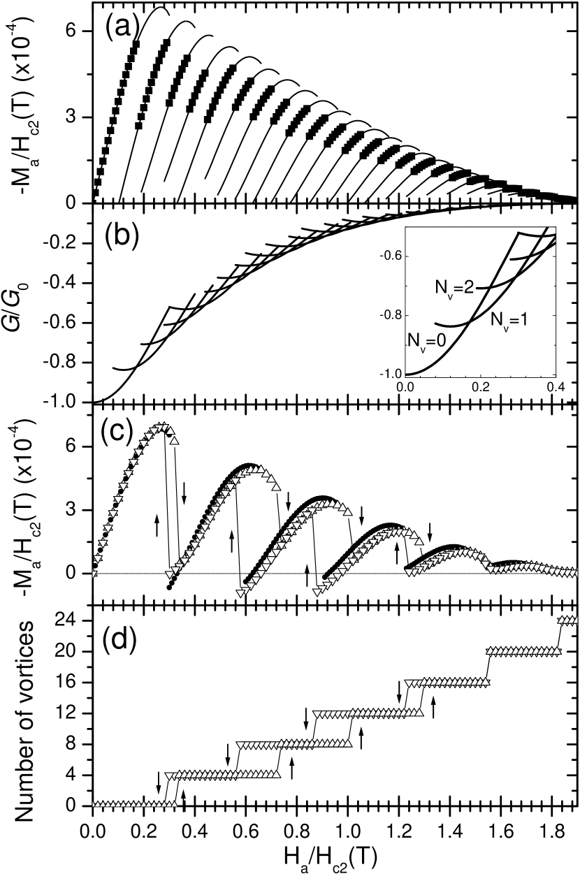
Figure 1: Results at $G_{i}=0$ and $T=0$. (a) The squares (${\scriptstyle\blacksquare}$) show the apparent magnetization corresponding to the energy ground state and the straight lines the $M_{a}$ results of all the meta-stable states. (b) Gibbs free energy of the different vortex states, the inset is a zoom at low fields. Apparent magnetization (c) and the number of vortices (d) calculated with the TDGL equations, when increasing ($\vartriangle$) and decreasing ($\triangledown$) the external magnetic field. The arrows show the vortex transition with TDGL.

The square symbols in Fig. 1(a) give the results of the apparent magnetization, corresponding to the “ground state” (global minimum of the mean-field free energy) as calculated within the stationary GL theory. The ground state vortex transitions are found calculating the free energy of all the possible (meta-stable) vortex states that are shown in Fig. 1(b). The inset is a zoom of the free energy at low fields. The different branches correspond to different values of the total vorticity, $N_{v}=\frac{1}{\Phi_{o}}\oint(A+\frac{J_{s}}{|\Psi|^{2}})dl$. Then, according to the global minima of the free energy, the vorticity changes always by one unit ($\Delta N_{v}=1$).

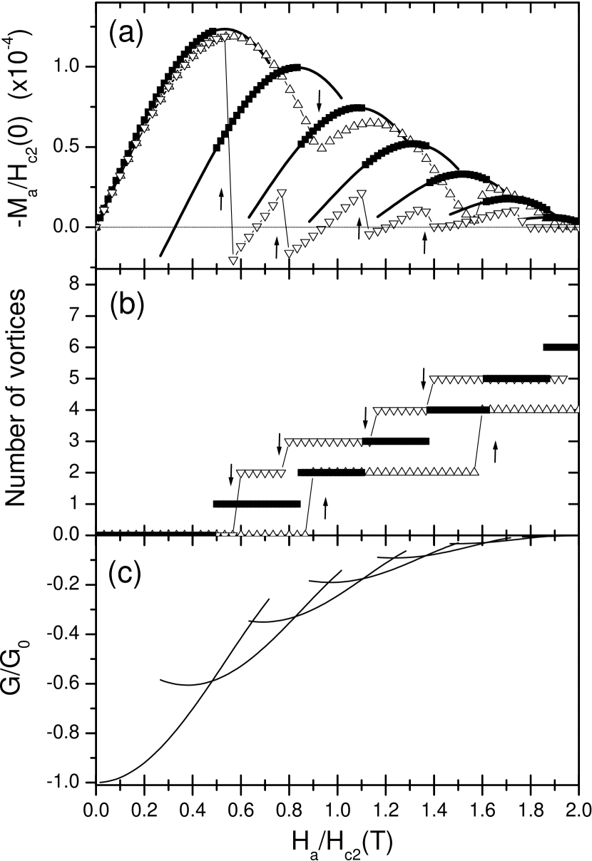
Figure 2: Similar results as Fig. 1 but now at $T=0.7T_{c}$ and $G_{i}=0$. (a) Apparent magnetization, $M_{a}$. The results obtained minimizing the mean-field GL free energy (${\scriptstyle\blacksquare}$) are compared to the dynamical results calculated with the TDGL equations, when increasing ($\vartriangle$) and decreasing ($\triangledown$) the external magnetic field. (b) The total vorticity vs. $H_{a}$ for the same cases as in (a). (c) Gibbs free energy of the different vortex states as a function of $H_{a}$.

In Fig. 1(c) we study the behavior of the apparent magnetization within the framework of the TDGL theory. The triangles show the behavior for increasing ($\vartriangle$) and decreasing ($\triangledown$) field. Notice that the transitions while increasing the field or decreasing the field do not occur at the same field values, i.e. the penetration field ($H_{p}$) differs from the expulsion field ($H_{e}$). This hysteresis is due to the surface barrier.PRB59 ; HD1 With increasing and decreasing field we see that the vorticity changes by four and minus four at the transitions, which means that the vortices enter or leave the sample by four, i.e. one vortex through each side of the square. This is shown more explicitly in Fig. 1(d) where the total vorticity, i.e. the number of vortices inside the sample, are plotted as a function of the applied magnetic field. Of course, following the ground state free energy, the vorticity changes always by one unit. The fact that in the TDGL results the vorticity changes by four at the transitions means that, in this case, there is not a simple dynamical path to break the square symmetry in the system during the field sweep. The close circles ($\bullet$) in Fig. 1(c) are the $-M_{a}/H_{c2}(T)$ values corresponding to the meta-stable states with vorticity equal to a multiple of four as calculated within the stationary GL theory. Notice that the values of $-M_{a}/H_{c2}(T)$ obtained using the TDGL and stationary GL theory are similar for the same number of vortices.

Next, we investigate the influence of finite temperature neglecting the thermal fluctuations, i.e. $G_{i}=0$. Figs. 2(a-c) show the same as Figs. 1(b-d), but now at temperature $T=0.7T_{c}$. When we increase the temperature, both $\xi(T)=\xi(0)/\sqrt{1-T/T_{c}}$ and $\lambda(T)=\lambda(0)/\sqrt{1-T/T_{c}}$ increase and the size of the sample decreases measured in units of $\xi(T)$, ($\xi(T=0.7T_{c})/\xi(0)=1.83$). In this case less vortex penetration events are necessary to arrive to the normal state. Notice that this is what happens in a typical experimental situation when the temperature is increased. The main difference with the zero-temperature situation is that in the present case the vorticity changes with $\Delta N_{v}=2$ for increasing magnetic field while the vorticity changes with $\Delta N_{v}=-1$ in most transitions for decreasing $H_{a}$. This behavior is different from the results obtained in Fig. 1(d) because of the small size of the sample as compared to $\xi(T)$. For example, in Fig. 2(b) we plot the number of vortices for increasing ($\vartriangle$) and decreasing ($\triangledown$) the magnetic field and we compare these results with the vorticity of the energy ground state (${\scriptstyle\blacksquare}$). The arrows show the vortex transitions with TDGL. In Fig. 2(b) we see the presence of hysteresis due to meta-stable states.

III.2 Thermal fluctuations

Next, we include thermal fluctuations, i.e. $G_{i}\neq 0$ in Eq. (10).

It is known that the free energy minima results obtained at temperature $T_{1}$ can be rescaled and will be equal to the free energy minima results of an “equivalent” system at a different temperature $T_{2}\neq T_{1}$. To be equivalent the systems must have the same size measured in units of $\xi(T)$ and the same $\kappa$. In Fig. 3(a) we compare the ground state apparent magnetization results for two situations: (i) a square with sides $W=10\xi(0)$ and thickness $d=0.1\xi(0)$ at $T=0$, and (ii) for a square with $W=10\xi(T)$ and $d=0.1\xi(T)$ at $T=0.7T_{c}$ for $G_{i}=10^{-10}$. As the size of the system is the same measured in $\xi(T)$ the latter results can be compared if we normalize the field by the temperature dependent $H_{c2}(T)$, as we did in Fig 3(a). We see that thermal fluctuations have broken the symmetry restrictions for vortex entrance and in this case $\Delta N_{v}=2$ for $H_{a}<0.8H_{c2}(T)$ and $\Delta N_{v}=1$ for $H_{a}>0.8H_{c2}(T)$, while $\Delta N_{v}=4$ when neglecting the thermal fluctuations (see Fig. 1(a)). Even when $\Delta N_{v}=1$, the dynamic TDGL results for $-M_{a}$ (open symbols) do not follow in detail the $-M_{a}$ curves obtained from free energy minimization (solid symbols). This behavior will be more clear in Fig. 3(b) in case of a smaller sample.

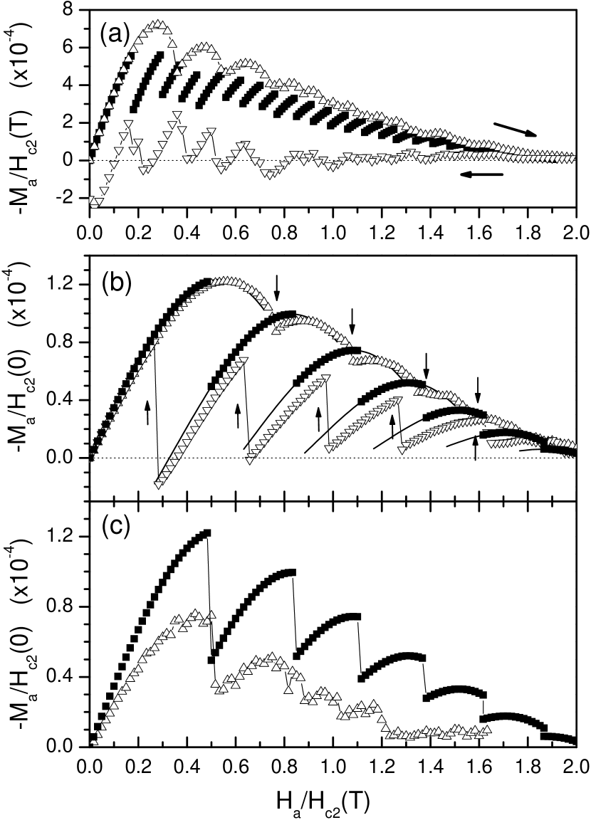
Figure 3: Results obtained including thermal fluctuations for $T=0.7T_{c}$. (a) $G_{i}=10^{-10}$, (b) $G_{i}=10^{-8}$ and (c) $G_{i}=10^{-5}$. The system size in (a) is $W=10\xi(T)$, $d=0.1\xi(T)$ and in (b) and (c) $W=10\xi(0)$, $d=0.1\xi(0)$. The triangles are for increasing ($\vartriangle$) and decreasing ($\triangledown$) the magnetic field and the solid squares are the results corresponding to the mean field ground states.

In Fig. 3(b) we show the apparent magnetization as a function of the applied magnetic field for a square with sides equal to $W=10\xi(0)$ and thickness $d=0.1\xi(0)$ at $T=0.7T_{c}$ for $G_{i}=10^{-8}$, i.e. a conventional low-$T_{c}$ superconductor. The square symbols and the solid curves are the apparent magnetization for the ground state and the meta-stable states as calculated within the framework of the stationary Ginzburg-Landau theory. The triangles indicate the results with increasing ($\vartriangle$) and decreasing ($\triangledown$) field when using the time-dependent Ginzburg-Landau theory, taking into account the thermal fluctuations. For this system size and $G_{i}=10^{-8}$ the TDGL results with increasing and decreasing magnetic field show that $\Delta N_{v}=1$. But, even though $\Delta N_{v}=1$, there is still hysteresis in the $-(M_{a})$ curve for such a conventional mesoscopic low-$T_{c}$ superconductor. The system clearly does not follow the mean field free energy minima behavior. Notice that there is a rather good agreement between the results from the TDGL theory and the stationary GL theory, both for the values of $-M_{a}$ and for the transition fields.

Even when the thermal fluctuations are weak, as in Fig. 3(b), it is expected that for a sufficient long simulation time the apparent magnetization would relax until the ground state is reached. In this case, the relaxation of the magnetic flux is related with the possibility that vortices overcome the surface barrier by thermal activation. In our simulations we allow the system to relax during 250000 time steps with $\Delta t=0.0045t_{o}$, which gives the system the possibility to relax during $t=1125\;t_{0}\sim 0.1\mu\mbox{sec}$. However, the hysteresis in the apparent magnetization curve is also observed experimentally GN390 in mesoscopic low-$T_{c}$ superconductors. Consequently, we can conclude that the half-life time of the meta-stable states is very large in low-$T_{c}$ superconductors even in comparison with the usual experimental times.

Next, we repeat the calculation for the same sample as in Fig. 3(b), but now including thermal fluctuations of strength corresponding to a high-$T_{c}$ superconducting material ($G_{i}=10^{-5}$). The results are shown in Fig. 3(c). We see that the first two penetration fields obtained from the TDGL equations agree very well with the ones resulting from the mean-field free energy minima. This means that the effect of the surface barrier is almost suppressed here, once we allow the system to relax a short time. On the other hand, the strong thermal fluctuations decrease the $-(M_{a})$ values in Fig. 3(c), with respect to the mean-field values. Below the first penetration field, in the Meissner state, the magnetic flux inside the sample ($BW^{2}$) depends only on the penetration length. Therefore, in the Meissner branch of figure Fig. 3(c) we can deduce from the slope of $M_{a}(H_{a})$ what appears to be an increase in $\lambda$ induced by thermal fluctuations. In fact, it is known that thermal fluctuations can induce an increase of the effective London penetration length in high-$T_{c}$ superconductors (see for example Ref. lobb, ), which is a consequence of the renormalization of the superfluid density due to thermal fluctuations, since $\lambda_{\mbox{eff}}^{2}=mc^{2}/(8\pi e^{2}\langle|\Psi|^{2}\rangle)$.

In order to understand these effects in Fig. 3(c), we investigate the time average of the order parameter $\langle|\Psi|^{2}\rangle$ and the time variations in the number of vortices ($N_{v}(t)$) for low and high-$T_{c}$ superconductors, with $G_{i}=10^{-8}$ and $G_{i}=10^{-5}$, respectively. In Figs. 4(a) and 4(c) we show $\langle|\Psi|^{2}\rangle$ along the x direction, i.e. from the middle of one side to the middle of the opposite side of the square, for two values of the applied magnetic field, $H_{a}=0.42H_{c2}(T)$ and $H_{a}=0.75H_{c2}(T)$. We obtain the following results: for $G_{i}=10^{-8}$ the number of vortices do not change in time and the $\langle|\Psi|^{2}\rangle(x)$ results (${\scriptstyle\blacksquare}$) are near to the mean field ones ($G_{i}=0$). However, for $G_{i}=10^{-5}$ we observe that $\langle|\Psi|^{2}\rangle(x)$ (${\scriptstyle\square}$) is lower than the mean field (MF) result and the number of vortices fluctuates in time.

The field $H_{a}=0.42H_{c2}(T)$, corresponds to the Meissner state without vortices in the mean-field case, see Fig. 3(b). For $G_{i}=10^{-8}$ we also obtain that $N_{v}(t)\equiv 0$ for all $t$. However, for $G_{i}=10^{-5}$ the number of vortices change in time. In Fig. 4(b) we plot a histogram of the different vortex states obtained during 250000 time steps. We see that the state with $N_{v}=0$ is the most probable one, but that there is also some probability to have jumps to other vortex states, mainly with $N_{v}=\pm 1$. Thus the reduction of $\langle|\Psi|^{2}\rangle$ from the mean field result for $G_{i}=10^{-5}$ is a consequence of thermal fluctuations which allow the nucleation of thermally induced vortex-antivortex pairs KT ; Beasley ; Hebard ; Kadin as well as the entrance and exit of thermally activated vortices. This leads to an increase of the effective $\lambda$, due to the lowering of $\langle|\Psi|^{2}\rangle$.

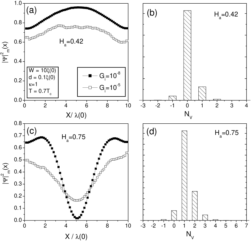
Figure 4: Time average of the order parameter in the $x$ direction, $|\Psi|^{2}_{m}$, for $G_{i}=10^{-8}$ (${\scriptstyle\blacksquare}$) and $G_{i}=10^{-5}$ (${\scriptstyle\square}$) for (a) $H_{a}=0.42H_{c2}(T)$ and (c) $H_{a}=0.75H_{c2}(T)$. (b) and (d) are histograms of the different vortex states obtained when $G_{i}=10^{-8}$.

Results similar to Figs. 4(a)-(b) are obtained in Figs. 4(c)-(d) for $H_{a}=0.75H_{c2}(T)$. Fig. 4(c) shows that, for $G_{i}=10^{-8}$ (${\scriptstyle\blacksquare}$), we have a vortex state with one vortex: $\langle|\Psi|^{2}\rangle=0$ in the center of the sample where the vortex is located. However, for $G_{i}=10^{-5}$(${\scriptstyle\square}$), we observe that $\langle|\Psi|^{2}\rangle(x)$ is different from zero in the center of the sample. The corresponding vortex state histogram is shown in Fig. 4(d). We see that the state with one vortex is the most probable one but that there is also a finite probability for other vortex states which contribute differently to $\langle|\Psi|^{2}\rangle$. This makes $\langle|\Psi|^{2}\rangle\neq 0$ in the center of the sample. There are continuous entrances and exits of vortices and the time average is a mixture of states with different vorticity.

More details about thermal activation of vortices can be obtained by calculating the average number of vortices $\langle N_{v}\rangle$:

$$\langle N_{v}\rangle=\frac{\Delta t}{t_{f}-t_{i}}\sum_{t=t_{i}}^{t_{f}}N_{v}(t)\;,$$ (27)

and the probability to have $N_{v}=n$ vortices ($P_{(N_{v}=n)}$):

$$P_{(N_{v}=n)}=\frac{\Delta t}{t_{f}-t_{i}}\sum_{t=t_{i}}^{t_{f}}\delta_{N_{v}(t);n}\;,$$ (28)

both magnitudes can be calculated if we know the number of vortices in each time step $N_{v}(t)$. Where the sum in Eqs. (27) and (28) are taken between two time values ($t_{i}$ and $t_{f}$), and $\delta_{N_{v}(t);n}$ is the Kronecker delta.

In Fig. 5(a) we plot the average number of vortices and in Fig. 5(b) the probabilities to find a specific vortex state as a function of the applied magnetic field. These results where obtained during the magnetic field sweep up shown in Fig. 3(c) ($G_{i}=10^{-5}$).

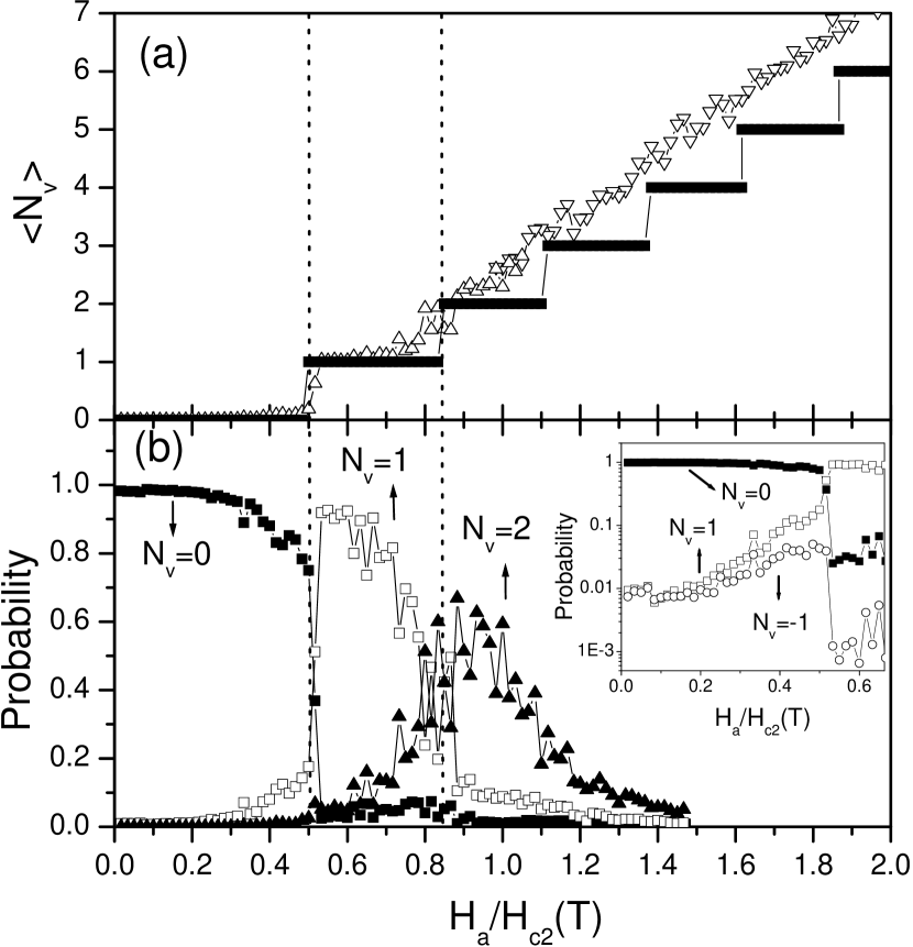
Figure 5: (a) Time average of the different vortex states obtained for $G_{i}=10^{-5}$ for increasing ($\vartriangle$) and decreasing ($\triangledown$) the magnetic field. The black squares (${\scriptstyle\blacksquare}$) are the ground state results. (b) Probability of the different vortex states. The inset is a zoom at low fields in a logarithmic scale.

In Fig. 5(a), for $G_{i}=10^{-5}$ ($\vartriangle$) and small magnetic fields ($H_{a}<0.7H_{c2}(T)$), we see that $\langle N_{v}\rangle$ vs. $H_{a}$ follows the mean field result ($N_{v}^{MF}(H_{a})$) (${\scriptstyle\blacksquare}$). For $H_{a}>0.7H_{c2}(T)$ the results are different, except at the start of each step where $\langle N_{v}\rangle=N_{v}^{MF}$. For strong thermal fluctuations we see that the average number of vortices can change continuously and is frequently larger than $N_{v}^{MF}$.

More details about the thermal activation of vortices can be obtained calculating the probability to have $N_{v}$ vortices using Eq. (28). In Fig. 5(b) we show the probabilities of the different vortex states for $G_{i}=10^{-5}$. The inset is a zoom of the low magnetic field region in a logarithmic scale. Near $H_{a}=0$, the probability of the zero vortex state is near one ($P_{(N_{v}=0)}\approx 1$) and we also see that $P_{(N_{v}=1)}\approx P_{(N_{v}=-1)}\approx 0.01$. From the inset we find that for $H_{a}\approx 0.5H_{c2}(T)$ there is a discontinuous jump down in $P_{(N_{v}=0)}$ and that at the same time the probability of having $N_{v}=1$ increases abruptly. When this happens we see that $\langle N_{v}\rangle=1$ in Fig. 5(a).

We also calculated the fluctuations in the vorticity ($N_{v}(t)$) and the fluctuations in $-M_{a}(t)/H_{c2}(0)$. The fluctuations in the magnitude of the apparent magnetization $M_{a}(t)$ is obtained through the relation:

$$\Delta M_{a}=\sqrt{\langle M_{a}^{2}\rangle-\langle M_{a}\rangle^{2}}\;\;,$$ (29)

where the mean values of $M_{a}$ (i.e. $\langle M_{a}\rangle$ and $\langle M_{a}^{2}\rangle$) are calculated using the definition given in Eq. (27).

Figure 6: (a) Fluctuations in the number of vortices and (b) in $-M_{a}/H_{c2}(0)$ for $G_{i}=10^{-5}$ corresponding to the situation of Fig. 5.

The fluctuations are shown in Fig. 6. From Fig. 6(a) we see that the fluctuations in the vorticity increase with increasing field until the first penetration field, $H_{p1}$, (first dashed vertical line), where there is a remarkable decrease in the number of vortex fluctuations. The fluctuations in $M_{a}$ also decrease at $H_{p1}$ as we can see from Fig. 6(b). At the second penetration field (second dashed line) in Fig. 6 the decrease in the fluctuations at $H_{p2}$ is almost completely buried under the thermal noise due to a continuous increase in the fluctuations of the number of vortices with increasing field, as seen in Fig. 6(a).

IV Conclusions

We studied the influence of the strength of thermal fluctuations on the magnetic behavior of mesoscopic superconductors. In the absence of thermal fluctuations and surface imperfections, we found that the vorticity changes by four at the transition fields due to the symmetry of the mesoscopic square sample. The surface barriers and the symmetry of the sample produce hysteresis and meta-stable states.

In low-$T_{c}$ mesoscopic superconductors, where thermal fluctuations are small, we did not find thermally activated entrance/exit of vortices through surface barriers. This result agrees with experiments in low-$T_{c}$ superconductors where hysteresis in the penetration fields and meta-stable states were found.

In low-$T_{c}$ superconductors, small thermal fluctuations however are enough to break the square symmetry restriction to vortex entrance and less vortices penetrate at the same field.

A different behavior was found when the strength of thermal fluctuations is increased as is the case for high-$T_{c}$ superconductors. In this case there are frequent thermally activated events of entrance/exit of vortices in agreement with recent experimental results on micron-sized high-$T_{c}$ superconducting thin film rings kogan-clem . We also found that thermal fluctuations increase the effective London penetration depth if we compare it with the mean field result.

In high temperature superconductors, the $d$-wave symmetry of the ground state and the tetragonal symmetry of the underlying crystalline structure can have an important effect in some of their macroscopic properties. These have been modeled by phenomenological Ginzburg-Landau or London theories, containing mixed gradient couplings to an order parameter with a different symmetry berlinsky ; heeb or additional quartic derivative nonlocal terms.ichioka ; kogan An important consequence of this is that, at large magnetic fields, the equilibrium vortex lattice deviates from the triangular Abrikosov lattice to a square lattice, as it has been observed recently.brown Also the possible effects in the individual structure of vortices in cuprates superconductors has been the subject of intense research.hoffman In the case of mesoscopic high-$T_{c}$ superconductors, the structure of the vortex configurations confined within the geometry of the sample and the quantitative values of the surface barrier and penetration fields could be affected by such considerations. On the other hand, the qualitative physics of the thermally activated entrance/exit of vortices through surface barriers should remain similar to the one described here with the dynamics of the simple GL equations. In any case, more experimental and theoretical works in this field are necessary. Therefore, the study of the physical properties of mesoscopic high-$T_{c}$ superconductors can contribute to the global understanding of these interesting materials.

V Acknowledgments

This work was supported by the Argentina-Belgium collaboration programme SECYT-FWO FW/PA/02-EIII/002. DD and ADH acknowledge support from ANPCYT PICT99-03-06343, from CONICET and from CNEA P5-PID-93-7. FMP and BJB acknowledge support from the Flemish Science Foundation (FWO-Vl) and the Belgian Science policy. B. J. Baelus also acknowledges support from the Japan Society for the Promotion of Science and FWO-Vl. A. D. Hernández also acknowledges support from the Centro Latinoamericano de Física and Fundación Antorchas.

References

- (1) V. V. Moshchalkov, L. Gielen, C. Strunk, R. Jonckheere, X. Qiu, C. Van Haesendonck, and Y. Bruynseraede, Nature (London) 373, 319 (1995).
- (2) V. Bruyndoncx, L. Van Look, M. Verschuere, and V. V. Moshchalkov, Phys. Rev. B 60, 10468 (1999).
- (3) L. F. Chibotaru, A. Ceulemans, V. Bruyndoncx, and V. V. Moshchalkov, Nature (London) 408, 833 (2000).
- (4) L. F. Chibotaru, A. Ceulemans, V. Bruyndoncx, and V. V. Moshchalkov, Phys. Rev. Lett. 86, 1323 (2001).
- (5) A. K. Geim, I. V. Grigorieva, S. V. Dubonos, J. G. S. Lok, J. C. Maan, A. E. Filippov, and F. M. Peeters, Nature (London) 390, 259 (1997).
- (6) A. K. Geim, S. V. Dubonos, J. G. S. Lok, M. Henini, and J. C. Maan, Nature (London) 396, 144 (1998).
- (7) A. K. Geim, S. V. Dubonos, I. V. Grigorieva, K. S. Novoselov, F. M. Peeters, and V. A. Schweigert, Nature (London) 407, 55 (2000).
- (8) S. Pedersen, G. R. Kofod, J. C. Hollingbery, C. B. Sørensen, and P. E. Lindelof, Phys. Rev. B 64, 104522 (2001).
- (9) A. Kanda, B. J. Baelus, F. M. Peeters, K. Kadowaki, and Y. Ootuka, Phys. Rev. Lett. 93, 257002 (2004).
- (10) B. J. Baelus, A. Kanda, F. M. Peeters, Y. Ootuka, and K. Kadowaki (unpublished).
- (11) V. A. Schweigert and F. M. Peeters, Phys. Rev. B 57, 13817 (1998).
- (12) V. A. Schweigert, F. M. Peeters, and P. S. Deo, Phys. Rev. Lett. 81, 2783 (1998).
- (13) V. A. Schweigert and F. M. Peeters, Phys. Rev. Lett. 83, 2409 (1999).
- (14) P. S. Deo, V. A. Schweigert, and F. M. Peeters, Phys. Rev. B 59, 6039 (1999).
- (15) J. J. Palacios, Phys. Rev. Lett. 84, 1796 (2000).
- (16) F. M. Peeters, B. J. Baelus, and V. A. Schweigert, Physica C 369, 158 (2002).
- (17) B. J. Baelus and F. M. Peeters, Phys. Rev. B 65, 104515 (2002).
- (18) A. D. Hernández and D. Domínguez, Phys. Rev. B 65, 144529 (2002).
- (19) A. D. Hernández and D. Domínguez, Phys. Rev. B 66, 144505 (2002).
- (20) M. Konczykowski, L. I. Burlachkov, Y. Yeshurun, and F. Holtzberg, Phys. Rev. B 43, R13707 (1991).
- (21) L. Burlachkov, V. B. Geshkenbein, A. E. Koshelev, A. I. Larkin, and V. M. Vinokur, Phys. Rev. B 50, R16770 (1994).
- (22) A. Schilling, R. Jin, J. D. Guo, and H. R. Ott, Phys. Rev. Lett. 71, 1899 (1993).
- (23) L. Civale, T. K. Worthington, and A. Gupta, Phys. Rev. B 48, 7576 (1993).
- (24) M. Niderost, R. Frassanito, M. Saalfrank, A. C. Mota, G. Blatter, V. N. Zavaritsky, T. W. Li, and P. H. Kes, Phys. Rev. Lett. 81, 3231 (1998).
- (25) Y. M. Wang, A. Zettl, S. Ooi, and T. Tamegai, Phys. Rev. B 65, 184506 (2002).
- (26) J. R. Kirtley, C. C. Tsuei, V. G. Kogan, J. R. Clem, H. Raffy, and Z. Z. Li, Phys. Rev. B 68, 214505 (2003).
- (27) Y. Enomoto and K. Okada, J. Phys.: Condens. Matter 9, 10203 (1997).
- (28) P. C. Hohenberg and B. I. Halperin, Rev. Mod. Phys. 49, 435 (1977).
- (29) W. D. Groop, H. G. Kaper, G. L. Leaf, D. M. Levine, M. Palumbo, and V. M. Vinokur, J. Comp. Phys. 123, 254 (1996).
- (30) R. Kato, Y. Enomoto, and S. Maekawa, Phys. Rev. B 47, 8016 (1993).
- (31) V. L. Ginzburg, Soviet Phys.-Solid St. 2, 1824 (1960).
- (32) G. Blatter, M. V. Feigel’man, V. B. Geshkenbein, A. I. Larkin, and V. M. Vinokur, Rev. Mod. Phys. 66, 1125 (1994).
- (33) E. H. Brandt, Phys. Rev. B 46, 8628 (1992); ibid., Phys. Rev. B 52, 15442 (1995).
- (34) A. D. Hernández and D. Domínguez, preprint cond-mat/0412631.
- (35) J. D. Jackson, Classical Electrodynamics (Wiley, New York, 1980).
- (36) D. Domínguez and J. V. Jose, Phys. Rev. B 53, 11 692 (1996).
- (37) C. J. Lobb, Phys. Rev. B 36, 3930 (1987).
- (38) J. M. Kosterlitz and D. J. Thouless, J. Phys. C 6, 1181 (1973).
- (39) M. R. Beasley, J. E. Mooij, and T. P. Orlando, Phys. Rev. Lett. 42, 1165 (1979).
- (40) A. F. Hebard and A. T. Fiory, Phys. Rev. Lett. 44, 291 (1980).
- (41) A. M. Kadin, K. Epstein, and A. M. Goldman, Phys. Rev. B 27, 6691 (1983).
- (42) A. J. Berlinsky, A. L. Fetter, M. Franz, C. Kallin, and P. I. Soininen, Phys. Rev. Lett. 75, 2200 (1995); M. Franz, C. Kallin, P. I. Soininen, A. J. Berlinsky, and A. L. Fetter Phys. Rev. B 53, 5795 (1996).
- (43) R. Heeb, A. van Otterlo, M. Sigrist, and G. Blatter, Phys. Rev. B 54, 9385 (1996).
- (44) M. Ichioka, N. Enomoto, N. Hayashi, and K. Machida Phys. Rev. B 53, 2233 (1996); M. Ichioka, N. Hayashi, N. Enomoto, and K. Machida, Phys. Rev. B 53, 15316 (1996); M. Ichioka, A. Hasegawa, and K. Machida, Phys. Rev. B 59, 8902 (1999).
- (45) V. G. Kogan, A. Gurevich, J. H. Cho, D. C. Johnston, Ming Xu, J. R. Thompson, and A. Martynovich Phys. Rev. B 54, 12386 (1996); V. G. Kogan, P. Miranovic, Lj. Dobrosavljevic-Grujic, W. E. Pickett, and D. K. Christen Phys. Rev. Lett. 79, 741 (1997); M. Franz, I. Affleck, and M. H. S. Amin Phys. Rev. Lett. 79, 1555 (1997)
- (46) S. P. Brown, D. Charalambous, E. C. Jones, E. M. Forgan, P. G. Kealy, A. Erb, and J. Kohlbrecher, Phys. Rev. Lett. 92, 067004 (2004).
- (47) I. Maggio-Aprile, Ch. Renner, A. Erb, E. Walker, and O. Fischer, Phys. Rev. Lett. 75, 2754(1995); J. E. Hoffman, E. W. Hudson, K. M. Lang, V. Madhavan, H. Eisaki, S. Uchida, and J. C. Davis, Science 295, 466 (2002).