Slave particle approach to the finite temperature properties of ultracold Bose gases in optical lattices

Abstract

By using slave particle (slave boson and slave fermion) technique on the Bose-Hubbard model, we study the finite temperature properties of ultracold Bose gases in optical lattices. The phase diagrams at finite temperature are depicted by including different types of slave particles and the effect of the finite types of slave particles is estimated. The superfluid density is evaluated using the Landau second order phase transition theory. The atom density, excitation spectrum and dispersion curve are also computed at various temperatures, and how the Mott-insulator evolves as the temperature increases is demonstrated. For most quantities to be calculated, we find that there are no qualitatively differences in using the slave boson or the slave fermion approaches. However, when studying the stability of the mean field state, we find that in contrast to the slave fermion approach, the slave boson mean field state is not stable. Although the slave boson mean field theory gives a qualitatively correct phase boundary, it corresponds to a local maximum of Landau free energy and can not describe the second order phase transition because the coefficient $a_{4}$ of the fourth order term is always negative in the free energy expansion.

I Introduction

Ultracold atoms in optical lattices with highly tunable parameters have provided an unique opportunity to simulate strongly correlated phenomena in condensed matter physics Bloch ; gre ; orzel . The dynamics of such Bose atoms can be described by a Bose-Hubbard model, and it was predicted that there would be a quantum phase transition from the superfluid to the Mott-insulator phase induced by varying the depth of the optical potential Jaksch . Recently, this phase transition has been perfectly realized by Greiner et al. gre by means of loading ⁸⁷Rb atoms into a three-dimensional optical lattices. From then on the Bose-Hubbard model to the cold atomic gas in optical lattices has received extensive studies.

The Bose-Hubbard model, with on-site interaction and tunnelling between nearest neighbor sites, was used by Fisher et. al fisher to investigate the bosons in periodic and/or random external potentials. There exist two types of phases, the superfluid and Mott-insulating phases, in this model at an integer lattice filling fraction and zero temperature. In the superfluid phase, the tunnelling term dominates and all atoms occupy the identical extended Bloch state. The ground state of this system can be well described by a macroscopic wave function with long-range phase coherence. In the Mott-insulating phase, the interaction dominates and the ground state of the system instead consists of the localized atomic wave function without phase coherence gre . This Mott-insulating phase can be characterized by an integer filling factor, the existence of a gap for particle-hole excitation, and zero compressibility. By varying the parameters such as the density and the external potential, the system would undergo a quantum phase transition and evolve from the superfluid phase to Mott-insulating phase. In the past, various theoretical approaches have been used to investigate this superfluid/Mott-insulator transition at zero temperature such as the strong-coupling expansion freericks ; freericks2 ; seng ; Elstner , Gutzwiller projection ansatz Jaksch ; Rokhsar ; Krauth ; Schroll , quantum Monte Carlo simulations Wessel ; numerical , and other mean-field approximations fisher ; oosten ; Sheshardi . By comparison, there are less studies focusing on the nonzero temperature properties D ; pv ; yy ; Sheshardi ; finiteT ; Konabe , and this will be the main topic of this paper.

Slave boson technique was developed to deal with the interacting fermion systems for the convenient use of mean-field approximations Kotliar . It has been extended to study the hard-core bosons on a lattice in a functional integral representation by Ziegler ziegler , in which there are only two states per site: empty and singly occupations. A similar formulation for interacting boson systems has been obtained by Frésard fresard . The analytical expression for the Mott-insulating lobes was obtained and the density-density correlation function was calculated. Recently, this approach has been adopted by Dicherscheid et al. D to investigate the nonzero temperature behaviors of the ultracold atoms in optical lattices. These authors showed that the calculated phase diagram at zero temperature agrees well with the results by other mean field methods freericks ; oosten and they further depicted the phase diagrams at finite temperatures. The slave boson and slave fermion approaches are equivalent in principle without any approximation. However, the difference comes into view if some mean field approximations are made in practical calculations. Bearing this in mind, one of us with Chui yy performed a comparative study between the slave fermion and slave boson approaches under the same mean-field approximation. It was found that both approaches give the same qualitative phase diagram, but the quantitative behaviors by slave fermion approach are more accurate. This may be related to the Fermi statistics which automatically excludes two same types of slave fermions from occupying the same site when the constraint, one site can be occupied by only one slave particle, is relaxed in the mean field approximation.

In this paper, we will extend the slave particle technique to investigate the various finite temperature properties of the Bose-Hubbard model. We will study the finite temperature phase diagram, atom density, superfluid density, and excitation spectrum for various temperatures and system parameters. The comparison between slave fermion and slave boson approaches will be performed. We show that although the mean field theory of slave boson gives a qualitatively reasonable phase boundary, the negative coefficient $a_{4}$ of fourth order term in the Landau free energy expansion means that the zero of the derivative of the free energy is a local maximum and thus the slave boson mean field state is not stable, i.e., the slave boson mean field theory is unable to describe the second order phase transition of the normal liquid/superfluid. This shortcoming of the slave boson approach does not exist in the slave fermion approach. In this sense, using the slave fermion approach to study the strongly correlated Bose atoms may be preponderant.

This paper was organized as follows. In Sec. II we review the basic formalism of the slave particle technique to the Bose-Hubbard model. In Sec. III we focus on the critical temperature of superfluid-normal phase transition, and depict the phase diagram. The atom density and the compressibility are calculated in Sec. IV. In Sec. V, the superfluid density is determined and the stability of the mean field states of the slave particles are discussed. Sec. VI is devoted to calculate the excitation spectrum. Conclusions are given in Sec. VII. In Appendix A, the details of the calculation of the coefficient $a_{4}$ is provided.

II Slave particle formalism of Bose-Hubbard model

II.1 Slave particle technique for a bosonic system

For a bosonic system, the creation operator $a_{i}^{{\dagger}}$ and annihilation operator $a_{i}$ on site $i$ can be defined as follows in the occupation-number representation:

$$a_{i}^{{\dagger}}|\alpha\rangle_{i}=\sqrt{\alpha+1}|\alpha+1\rangle_{i},$$

$$a_{i}|\alpha\rangle_{i}=\sqrt{\alpha}|\alpha-1\rangle_{i}.$$ (1)

They obey the basic boson commutation relation: $[a_{i},a_{j}^{{\dagger}}]=\delta_{ij}$. The state $|\alpha\rangle_{i}$ is an eigenstate of the particle number operator $N_{i}=a_{i}^{{\dagger}}a_{i}$, which counts the number of bosons on site $i$, with the eigenvalue $\alpha$. On a single lattice site, the occupation number can be any non-negative integer. Thus the boson creation and annihilation operators can be decomposed into

$$a_{i}^{\dagger}=|1\rangle_{ii}\langle 0|+\sqrt{2}|2\rangle_{ii}\langle 1|+\cdots=\sum_{\alpha=0}\sqrt{\alpha+1}|\alpha+1\rangle_{ii}\langle\alpha|,$$

$$a_{i}=|0\rangle_{ii}\langle 1|+\sqrt{2}|1\rangle_{ii}\langle 2|+\cdots=\sum_{\alpha=0}\sqrt{\alpha+1}|\alpha\rangle_{ii}\langle\alpha+1|.$$ (2)

The justification of this decomposition is that it does satisfy the original commutation relation $[a_{i},a_{j}^{{\dagger}}]=\delta_{ij}$. Next, we identify every occupation state on a site as a type of slave particle, that is to say, mapping $|\alpha\rangle_{i}$ and ${}_{i}\langle\alpha|$ to the creation operator $a_{\alpha,i}^{{\dagger}}$ and annihilation operator $a_{\alpha,i}$ of the slave particle. In a slave fermion approach these operators are forced to satisfy the fermion anticommutation relation $\{a_{\alpha,i},a_{\beta,j}^{\dagger}\}=\delta_{\alpha\beta}\delta_{ij}$, and in a slave boson approach they are forced to obey boson commutation relation $[a_{\alpha,i},a_{\beta,j}^{\dagger}]=\delta_{\alpha\beta}\delta_{ij}$. Then $a_{i}^{{\dagger}}$ and $a_{i}$ can be rewritten as

$$\begin{split}a_{i}^{{\dagger}}=\sum_{\alpha=0}\sqrt{\alpha+1}a_{\alpha+1,i}^{{\dagger}}a_{\alpha,i},\\ a_{i}=\sum_{\alpha=0}\sqrt{\alpha+1}a_{\alpha,i}^{{\dagger}}a_{\alpha+1,i}.\end{split}$$ (3)

When inserting the above equations in $[a_{i},a_{j}^{{\dagger}}]$, one finds that, only when the constraint

$$\sum_{\alpha=0}n_{i}^{\alpha}=\sum_{\alpha=0}a_{\alpha,i}^{{\dagger}}a_{\alpha,i}=1,$$ (4)

is satisfied, could the original boson commutation relation $[a_{i},a_{j}^{{\dagger}}]=\delta_{ij}$ be reproduced by either slave fermion or slave boson approaches. This implies that the slave particle transformation (3) along with the constraint (4) and $\{a_{\alpha,i},a_{\beta,j}^{\dagger}\}=\delta_{\alpha\beta}\delta_{ij}$ (slave fermion) or $[a_{\alpha,i},a_{\beta,j}^{\dagger}]=\delta_{\alpha\beta}\delta_{ij}$ (slave boson) can describe the whole physics of the original boson system.

II.2 Bose-Hubbard model and functional integral representation

In the second quantization, the translationally invariant many-body Hamiltonian of cold Bose gases confined by an external optical lattice potential $V_{ext}(\textbf{r})$ is given by dalfovo ,

$$\begin{split}H=&\int{d\textbf{r}\Psi^{\dagger}(\textbf{r})\left(-\frac{\hbar^{2}}{2m}\nabla^{2}+V_{ext}(\textbf{r})-\mu\right)\Psi(\textbf{r})}\\ &+\frac{1}{2}\int{d\textbf{r}d\textbf{r}^{\prime}\Psi^{\dagger}(\textbf{r})\Psi^{\dagger}(\textbf{r}^{\prime})V(\textbf{r}-\textbf{r}^{\prime})\Psi(\textbf{r}^{\prime})\Psi(\textbf{r})},\end{split}$$ (5)

where $\Psi(\textbf{r})$ ($\Psi^{\dagger}(\textbf{r})$) is the boson field operator that annihilates (creates) a particle at the position r, $V(\textbf{r}-\textbf{r}^{\prime})$ is the two-body interatomic potential, and $\mu$ is the chemical potential. In the case of a dilute cold atom gas, we can approximate $V(\textbf{r}-\textbf{r}^{\prime})$ with an effective interaction $g\delta(\textbf{r}-\textbf{r}^{\prime})$, where $g=4\pi{a_{s}}\hbar^{2}/m$ with $a_{s}$ the s-wave scattering length and $m$ the mass of the atoms. When expanding the field operators in the Wannier basis and keeping only the lowest vibrational states, namely $\Psi(\textbf{r})=\sum_{i}a_{i}w(\textbf{r}-\textbf{r}_{i})$, eq. (5) can be rewritten as the Bose-Hubbard Hamiltonian Jaksch :

$$H=-t\sum_{<ij>}a^{\dagger}_{i}a_{j}-\mu\sum_{i}n_{i}+\frac{U}{2}\sum_{i}n_{i}(n_{i}-1),$$ (6)

in which $n_{i}=a_{i}^{\dagger}{a_{i}}$ is the particle number operator. The symbol $\langle{ij}\rangle$ denotes the sum over all nearest neighbor sites. $t$ and $U$ are the hopping amplitude and on-site interaction, respectively,

$$t = \int{d\textbf{r}w^{*}(\textbf{r}-\textbf{r}_{i})\left(-\frac{\hbar^{2}}{2m}\nabla^{2}+V_{ext}(\textbf{r})\right)w(\textbf{r}-\textbf{r}_{j})},$$

$$U = g\int{d\textbf{r}|w(\textbf{r})|^{4}}.$$ (7)

For small occupation per site, one can use the single particle Wannier function to calculate these parameters. However, in the case of the multi-occupation, these parameters have to be calculated by considering the interaction broadening of the Wannier function jinbin . Substituting eq. (3) into eq. (6), the Bose-Hubbard Hamiltonian can be replaced by

$$\begin{split}H=&-t\sum_{<ij>}\sum_{\alpha,\beta}\sqrt{\alpha+1}\sqrt{\beta+1}a_{\alpha+1,i}^{{\dagger}}a_{\alpha,i}a_{\beta,j}^{{\dagger}}a_{\beta+1,j}\\ &-\mu\sum_{i}\sum_{\alpha}{\alpha}n_{i}^{\alpha}+\frac{U}{2}\sum_{i}\sum_{\alpha}\alpha(\alpha-1)n_{i}^{\alpha}.\end{split}$$ (8)

Following the steps in Refs. negele ; stoof , we write the partition function as an imaginary time coherent state path integral:

$$Z={\rm Tr}e^{-{\beta}H}=\int{Da_{\alpha}D\bar{a}_{\alpha}D{\lambda}e^{-S[\bar{a}_{\alpha},a_{\alpha},\lambda]}},$$

$$S[\bar{a}_{\alpha},a_{\alpha},\lambda]=\int_{0}^{\beta}{d\tau}\biggl{\{}\sum_{i}\sum_{\alpha}\bar{a}_{\alpha,i}[\partial_{\tau}-\alpha\mu+\frac{U}{2}\alpha(\alpha-1)-i\lambda_{i}]a_{\alpha,i}$$

$$+i\sum_{i}\lambda_{i}-t\sum_{<ij>}\sum_{\alpha,\beta}\sqrt{\alpha+1}\sqrt{\beta+1}\bar{a}_{\alpha+1,i}a_{\alpha,i}\bar{a}_{\beta,j}a_{\beta+1,j}\biggr{\}},$$ (9)

where $\bar{a}_{\alpha,i}$ and $a_{\alpha,i}$ are introduced as ordinary complex numbers in the slave boson approach, and as Grassmann variables in the slave fermion approach satisfying the Grassmann algebra, i.e., $\{a_{\alpha},a_{\alpha}\}=\{a_{\alpha},\bar{a}_{\alpha}\}=\{\bar{a}_{\alpha},\bar{a}_{\alpha}\}$, $\int da_{\alpha}1=0$ and $\int da_{\alpha}a_{\alpha}=1$ negele ; stoof . The gaussian integrals over them are

$$\int{D}a_{\alpha}D\bar{a}_{\alpha}\exp\left\{-\sum_{\alpha\beta}\bar{a}_{\alpha}A_{\alpha\beta}a_{\beta}\right\}=(\det{A})^{\pm}=e^{{\pm}Tr[\ln{A}]},$$ (10)

where $\pm$ correspond to integral over Grassmann variables or ordinary complex numbers. The Lagrange multiplier field $\lambda_{i}(\tau)$ comes from the constraint (4), namely, $\prod_{i}\delta(\sum_{\alpha}n_{i}^{\alpha}-1)$. The unit has been set to $\hbar=k_{B}=1$ in all formulas. In order to decouple the hopping term, a Hubbard-Stratonovich transformation is performed by adding a complete square term to the action which contributes to the partition function a constant,

$$\begin{split}\int{D\Phi^{*}D\Phi}\exp&\left[-\int d\tau t\sum_{<ij>}(\Phi_{i}^{*}-\sum_{\alpha}\sqrt{\alpha+1}\bar{a}_{\alpha+1,i}a_{\alpha,i})\right.\\ &\left.\times(\Phi_{j}-\sum_{\alpha}\sqrt{\alpha+1}\bar{a}_{\alpha,j}a_{\alpha+1,j})\right].\end{split}$$ (11)

Then the partition function is replaced by

$$\begin{split}Z&=\int{D\Phi^{*}D\Phi D\bar{a}_{\alpha}Da_{\alpha}D{\lambda}e^{-S_{eff}[\Phi,a_{\alpha},\lambda]}},\\ S_{eff}[\Phi,a_{\alpha},\lambda]&=\int_{0}^{\beta}{d\tau}\left\{\sum_{i}\sum_{\alpha}\bar{a}_{\alpha,i}\left[\partial_{\tau}-\alpha\mu+\frac{U}{2}\alpha(\alpha-1)-i\lambda_{i}\right]a_{\alpha,i}\right.\\ &\left.+i\sum_{i}\lambda_{i}+t\sum_{<ij>}(\Phi_{i}^{*}\Phi_{j}-\Phi_{i}^{*}\sum_{\alpha}\sqrt{\alpha+1}\bar{a}_{\alpha,j}a_{\alpha+1,j}\right.\\ &\left.-\Phi_{j}\sum_{\alpha}\sqrt{\alpha+1}\bar{a}_{\alpha+1,i}a_{\alpha,i})\right\}.\\ \end{split}$$ (12)

The Hubbard-Stratonovich field $\Phi_{i}$ introduced here can be identified as the order parameter of superfluid for $\langle\Phi_{i}\rangle=\langle\sum_{\alpha}\sqrt{\alpha+1}\bar{a}_{\alpha,i}a_{\alpha+1,i})\rangle=\langle{a_{i}}\rangle$. We then perform a Fourier transform on the field $A_{i}$:

$$\begin{split}A_{i}=\frac{1}{\sqrt{L\beta}}\sum_{\textbf{k},n}A_{\textbf{k}n}e^{i(\textbf{k}\cdot{\textbf{r}_{i}}-\omega_{n}\tau)},\end{split}$$ (13)

where $L$ is the total number of sites in the optical lattice, $\omega_{n}$ is the Matsubara frequency, which equals $(2n+1)\pi/\beta$ and $2n\pi/\beta$ for fermion and boson fields, respectively. The effective action $S_{eff}$ now reads

$$\begin{split}S_{eff}[\Phi,a_{\alpha},\lambda]&=\sum_{\textbf{k},n}\sum_{\alpha}\bar{a}_{\alpha,\textbf{k}n}\left[-i\omega_{n}-\alpha\mu+\frac{U}{2}\alpha(\alpha-1)\right]a_{\alpha,\textbf{k}n}+i\sqrt{L\beta}\lambda_{\textbf{0},0}\\ &-i\frac{1}{\sqrt{L\beta}}\sum_{\textbf{k},\textbf{q},n,n^{\prime}}\sum_{\alpha}\lambda_{\textbf{q},n^{\prime}}\bar{a}_{\alpha,\textbf{k}n}a_{\alpha,(\textbf{k+q})(n+n^{\prime})}+\sum_{\textbf{k},n}\epsilon_{\textbf{k}}|\Phi_{\textbf{k},n}|^{2}\\ &-\sum_{\textbf{k},\textbf{k}^{\prime},n,n^{\prime}}\sum_{\alpha}\frac{\epsilon_{\textbf{k}^{\prime}}}{\sqrt{L\beta}}\left\{\left(\sqrt{\alpha+1}\bar{a}_{\alpha+1,(\textbf{k+k}^{\prime})(n+n^{\prime})}a_{\alpha,\textbf{k}n}\right)\Phi_{{\textbf{k}^{\prime},n^{\prime}}}\right.\\ &\left.+{\left(\sqrt{\alpha+1}\bar{a}_{\alpha,\textbf{k}n}a_{\alpha+1,(\textbf{k+k}^{\prime})(n+n^{\prime})}\right)\Phi_{{\textbf{k}^{\prime},n^{\prime}}}^{*}}\right\},\end{split}$$ (14)

where $\epsilon_{\textbf{k}}=2t\sum_{i=1}^{d}\cos({k_{i}}a)$ with $d$ and $a$ being the dimension and spacing constant of the lattice. So far, we have obtained an effective action in a functional integral representation by the slave particle approach. It is a reexpression of the original Bose-Hubbard model since all transformations we made are rigorous. This effective action is the starting point of our calculations.

II.3 Perturbation theory

The system can not be exactly solved with the constraint (4), which means there is exactly one type of slave particle per site Kotliar ; p.a.lee . We then relax it to one slave particle per site on average over the whole lattice. To realize this, one can replace all $\lambda_{\textbf{k},n}$ in the action (14) with a constant $\lambda_{\textbf{0},0}$. This approximation is widely used in dealing with the interacting fermion systems Kotliar ; p.a.lee . It implies that the multi-occupation of the slave particles on one site is allowed. However, the behaviors of the slave boson and slave fermion are slightly different in the relaxing process. The multi-occupation of the same type of slave boson is allowed, while the multi-occupation of the same type of slave fermion is forbidden by the Pauli principle yy . This will lead to some quantitative differences in the results by these two approaches.

According to the Landau phase transition theory, the order parameter $\Phi$ near the critical point is small and then the perturbation theory can be used. In the following, we will try to integrate the slave particle field out of the action (14), and perform perturbation calculation toward $\Phi$ along the way in Ref. D . After relaxing the constraint (4), the action (14) can be divided into two parts:

$$\begin{split}S_{eff}[\Phi,a_{\alpha},\lambda]=S_{0}+S_{I}\end{split}$$

$$\begin{split}S_{0}=iL\beta\lambda+\sum_{\textbf{k},n}\sum_{\alpha}\bar{a}_{\alpha,\textbf{k}n}\left[-i\omega_{n}+c(\alpha)\right]a_{\alpha,\textbf{k}n}+\sum_{\textbf{k},n}\epsilon_{\textbf{k}}|\Phi_{\textbf{k},n}|^{2}=S_{0}^{sp}+\sum_{\textbf{k},n}\epsilon_{\textbf{k}}|\Phi_{\textbf{k},n}|^{2}\end{split}$$

$$\begin{split}S_{I}=-\sum_{\textbf{k},\textbf{k}^{\prime},n,n^{\prime}}&\sum_{\alpha}\frac{\epsilon_{\textbf{k}^{\prime}}}{\sqrt{L\beta}}\left\{\left(\sqrt{\alpha+1}\bar{a}_{\alpha+1,(\textbf{k+k}^{\prime})(n+n^{\prime})}a_{\alpha,\textbf{k}n}\right)\Phi_{{\textbf{k}^{\prime},n^{\prime}}}\right.\\ &\left.+{\left(\sqrt{\alpha+1}\bar{a}_{\alpha,\textbf{k}n}a_{\alpha+1,(\textbf{k+k}^{\prime})(n+n^{\prime})}\right)\Phi_{{\textbf{k}^{\prime},n^{\prime}}}^{*}}\right\},\end{split}$$

in which $\lambda=\lambda_{\textbf{0},0}/\sqrt{L\beta}$ is a constant and

$$c(\alpha)=-i\lambda-\alpha\mu+\alpha(\alpha-1)\frac{U}{2}.$$ (15)

The partition function $Z_{0}$ of non-interacting slave particles comes from the contribution of the zeroth-order term $S^{sp}_{0}$ and is given by

$$Z_{0}=e^{-\beta\Omega_{0}}=\int{Da_{\alpha}D\bar{a}_{\alpha}e^{-S_{0}^{sp}}}$$ (16)

where $\Omega_{0}$ is the zeroth-order thermodynamic potential and has the form:

$$-\Omega_{0}=i\lambda{L}\pm\frac{L}{\beta}\sum_{\alpha}\ln(1\pm e^{-\beta c(\alpha)}),$$ (17)

where the $+(-)$ sign corresponds to the slave fermion (slave boson), respectively. Then we can define the average of an operator $A$ with respect to $S_{0}^{sp}$ as

$$\begin{split}\langle{A}\rangle_{0}=\frac{1}{Z_{0}}\int{Da_{\alpha}D\bar{a}_{\alpha}A(a_{\alpha},\bar{a}_{\alpha})e^{-S_{0}^{sp}}}.\end{split}$$ (18)

For small $\Phi$, $e^{-S_{eff}}$ can be expanded in terms of $S_{I}$ D ; stoof , i.e.,

$$\begin{split}e^{-S_{eff}}=e^{-(S_{0}+S_{I})}\approx{e^{-S_{0}}\left[1-S_{I}+\frac{1}{2}S_{I}^{2}\right]}.\end{split}$$ (19)

After integrating out the slave particle field $a_{\alpha}$ and $\bar{a}_{\alpha}$, we arrive at a new effective action $S_{E,eff}$,

$$e^{-S_{E,eff}}=\int{Da_{\alpha}D\bar{a}_{\alpha}e^{-S_{eff}}}=e^{-\beta\Omega_{0}-\sum_{\textbf{k},n}\epsilon_{\textbf{k}}|\Phi_{\textbf{k},n}|^{2}}\left[1-\langle{S_{I}}\rangle_{0}+\frac{1}{2}\langle{S_{I}^{2}}\rangle_{0}\right].$$ (20)

It is straightforward to calculate $\langle{S_{I}}\rangle_{0}$ and $\langle{S_{I}^{2}}\rangle_{0}$ using the Wick’s theorem and gaussian integral formula (eq. (10)),

$$\langle{S_{I}}\rangle_{0} = 0,$$ (21)

$$\langle{S_{I}^{2}}\rangle_{0} = \mp 2\sum_{\textbf{k},\textbf{k}^{\prime},n,n^{\prime}}\frac{\epsilon_{\textbf{k}^{\prime}}^{2}|\Phi_{{\textbf{k}^{\prime},n^{\prime}}}|^{2}}{L\beta}\sum_{\alpha}(\alpha+1)\langle{\bar{a}_{\alpha,\textbf{k}n}a_{\alpha,\textbf{k}n}}\rangle_{0}$$ (22)

$$\times\langle{\bar{a}_{\alpha+1,(\textbf{k+k}^{\prime})(n+n^{\prime})}a_{\alpha+1,(\textbf{k+k}^{\prime})(n+n^{\prime})}}\rangle_{0}$$

$$= \mp 2\sum_{\textbf{k},\textbf{k}^{\prime},n,n^{\prime}}\frac{\epsilon_{\textbf{k}^{\prime}}^{2}|\Phi_{{\textbf{k}^{\prime},n^{\prime}}}|^{2}}{L\beta}\sum_{\alpha}(\alpha+1)\frac{1}{-i\omega_{n}+c(\alpha)}$$

$$\times\frac{1}{-i\omega_{n+n^{\prime}}+c(\alpha+1)},$$

where $\mp$ correspond to the slave fermion and slave boson. After performing the sums over Matsubara frequency $\omega_{n}$ and k, we reduce $\langle{S_{I}^{2}}\rangle_{0}$ to

$$\begin{split}\langle{S_{I}^{2}}\rangle_{0}=&2\sum_{\textbf{k},n}\epsilon_{\textbf{k}}^{2}|\Phi_{{\textbf{k},n}}|^{2}\sum_{\alpha}(\alpha+1)\frac{n^{\alpha}-n^{\alpha+1}}{-i\omega_{n}-\mu+\alpha{U}},\end{split}$$ (23)

where $n^{\alpha}$ is the occupation number and equal to

$$n^{\alpha}=\frac{1}{\exp\{\beta[-i\lambda-\alpha\mu+\alpha(\alpha-1)U/2]\}\pm 1},$$ (24)

in which the $+$ and $-$ sign correspond to slave fermion and slave boson respectively. Because $\langle{S_{I}^{2}}\rangle_{0}$ is small, we have

$$\begin{split}\left[1-\langle{S_{I}}\rangle_{0}+\frac{1}{2}\langle{S_{I}^{2}}\rangle_{0}\right]=\left[1+\frac{1}{2}\langle{S_{I}^{2}}\rangle_{0}\right]\approx e^{\frac{1}{2}\langle{S_{I}^{2}}\rangle_{0}},\end{split}$$ (25)

and can rewrite eq. (20) as

$$e^{-S_{E,eff}}=e^{-\beta\Omega_{0}-\sum_{\textbf{k},n}\epsilon_{\textbf{k}}|\Phi_{\textbf{k},n}|^{2}+\frac{1}{2}\langle{S_{I}^{2}}\rangle_{0}}.$$ (26)

Then the effective action of the order parameter field $S_{E,eff}[\Phi^{*},\Phi]$ may be obtained

$$S_{E,eff}[\Phi^{*},\Phi]=\beta\Omega_{0}-\sum_{\textbf{k},n}\Phi^{*}_{\textbf{k},n}G^{-1}(\textbf{k},i\omega_{n})\Phi_{\textbf{k},n},$$ (27)

where the Green’s function $G(\textbf{k},i\omega_{n})$ is defined by

$$-G^{-1}(\textbf{k},i\omega_{n})=\epsilon_{\textbf{k}}-\epsilon_{\textbf{k}}^{2}\sum_{\alpha}(\alpha+1)\frac{n^{\alpha}-n^{\alpha+1}}{-i\omega_{n}-\mu+\alpha{U}},$$ (28)

which will be the starting point of our analysis.

II.4 Mean-field approximation

In terms of eq. (27), the partition function can be calculated by gaussian integral

$$\begin{split}Z=&e^{-\beta\Omega}=\int{D\Phi D\Phi^{*}e^{-S_{E,eff}}}\\ =&\int{{D\Phi}D\Phi^{*}e^{-\beta\Omega_{0}+\sum_{\textbf{k},n}\Phi^{*}_{\textbf{k},n}G^{-1}(\textbf{k},i\omega_{n})\Phi_{\textbf{k},n}}}\\ =&e^{-\beta\Omega_{0}-\sum_{\textbf{k},n}\ln[-{\beta}G^{-1}(\textbf{k},i\omega_{n})]},\end{split}$$ (29)

from which the thermodynamic potential $\Omega$ can be extracted:

$$\Omega=\Omega_{0}+\frac{1}{\beta}\sum_{\textbf{k},n}\ln[-{\beta}G^{-1}(\textbf{k},i\omega_{n})].$$ (30)

We then perform a saddle point approximation to the constraint field $\lambda$, which means that we only choose the $\lambda$ minimizing the thermodynamic potential: $\partial\Omega/\partial\lambda=0$. In addition, the particle number conservation condition requires $-\partial\Omega/\partial\mu=N$. When inserting eq. (30) into these two conditions, we have

$$\begin{split}L\sum_{\alpha}(1-n^{\alpha})-\frac{i}{\beta}\sum_{\textbf{k},n}G(\textbf{k},i\omega_{n})\frac{{\partial}G^{-1}(\textbf{k},i\omega_{n})}{\partial\lambda}=0,\\ L\sum_{\alpha}{\alpha}n^{\alpha}+\frac{1}{\beta}\sum_{\textbf{k},n}G(\textbf{k},i\omega_{n})\frac{{\partial}G^{-1}(\textbf{k},i\omega_{n})}{\partial\mu}=N.\end{split}$$ (31)

The mean-field approximation means the last terms of the above equations may be neglected. That is, all the fluctuations coming from the Green’s function would not be considered. Then the following two equations can be derived,

$$\sum_{\alpha=0}n^{\alpha}=1,$$ (32)

$$\sum_{\alpha=0}{\alpha}n^{\alpha}=\frac{N}{L}=n,$$ (33)

where the $n=N/L$ is the average particle density. One can see that eq. (32), which implies there is one slave fermion per site on average, is exactly the relaxed constrain (4).

III The superfluid-normal phase transition

As we know, the quantum phase transition from superfluid to Mott-insulator only occurs at $T=0$. At finite temperature, a superfluid-normal phase transition will be induced D ; yy ; pv ; ziegler . The Landau theory shows that, near the critical point of superfluid-normal phase transition, the order parameter of superfluid $\Phi$ is small and the Landau free energy can be expanded in terms of it. The critical point can be determined by the coefficient of the second order term $|\Phi|^{2}$, which is $G^{-1}(\textbf{0},0)=0$ in our case D ; yy . According to eq. (28) and noting that $\epsilon_{0}=zt$, we have

$$\sum_{\alpha=0}(\alpha+1)\frac{n^{\alpha+1}-n^{\alpha}}{\bar{\mu}-{\alpha}\bar{U}}=1,$$ (34)

where $\bar{\mu}=\mu/zt$ and $\bar{U}=U/zt$ are dimensionless chemical potential and on-site repulsion strength with $z$ being the number of nearest neighbors. The dimensionless critical temperature $\bar{T}_{c}=T_{c}/zt$ can be obtained by solving eqs. (24), (32), (33), and (34) together. Note that our results have a clear mean field nature and the dimensionality of the lattice appears only as a numerical factor. Because there are infinite types of slave particles, a cut-off toward $\alpha$ should be made when solving these equations. It has been shown by one of us and Chui yy that, for a large $\bar{U}$ a small cut-off (e.g. $\alpha_{M}=3$) is a good approximation, but in the region of small $\bar{U}$ the contributions from large $\alpha$ slave particles cannot be neglected and a larger $\alpha_{M}$ is required to obtain a quantitatively reliable result. In this work, we will work at a relative large $\alpha_{M}$ ( say, 9) to obtain a more accurate phase diagram of superfluid-normal transition and estimate the effect of the finite types of slave particles.

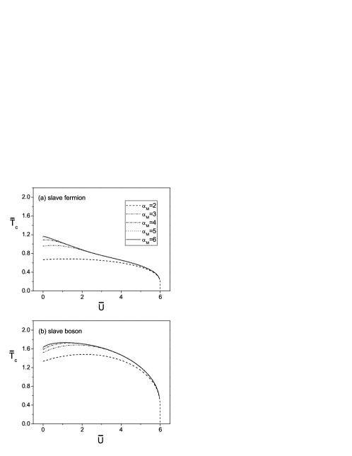
Figure 1: The superfluid-normal phase diagrams with various cut-off $\alpha_{M}$ in the slave fermion ((a)) and the slave boson ((b)) approaches. The average density is set to be $n=1$. $\bar{T}_{c}=T_{c}/zt$ and $\bar{U}=U/zt$ are the dimensionless critical temperature and on-site interaction, respectively.

When considering the commensurate state and restricting the average density to $n=N/L=1$, we obtain the superfluid-normal phase diagrams with various cut-off $\alpha_{M}$ in both slave fermion and slave boson approaches. It can be seen from Fig. 1 that, in both approaches, the curves of various cut-off are different from each other in the small $\bar{U}$ region. As $\bar{U}$ increases, these differences become small and disappear gradually when approaching the critical point of superfluid-Mott insulator transition. This result gives a further support to the statement of Ref. yy that more types of slave particles should be taken into account in the small $\bar{U}$ region. Moreover, we find that the $\bar{T}_{c}-\bar{U}$ curves with $\alpha_{M}>7$, which are not shown in Fig. 1, almost coincide with the curve with $\alpha_{M}=6$. This implies that even in the small $\bar{U}$ region the contributions from the slave particles with $\alpha>6$ can be reasonably neglected. To make the effect of finite cut-off $\alpha_{M}$ clearer, we plot the position of local maximum in the $\bar{T}_{c}-\bar{U}$ curve, denoted by $\bar{U}_{max}$, and the critical temperature at $\bar{U}=0$, denoted by $\bar{T}_{c0}$, as a function of $\alpha_{M}$ in Fig. 2. We can see that, as the cut-off $\alpha_{M}$ increases, the positions of local maximum $\bar{U}_{max}$ move to small $\bar{U}$ and approach steadily to 0 and 1.1 after $\alpha_{M}>6$ for the slave fermion and the slave boson, respectively. The critical temperatures $\bar{T}_{c0}$ shown in Fig. 2(b) initially increase largely when we increase the $\alpha_{M}$, but their dependencies on it become very small after $\alpha_{M}>6$ in both slave particle approaches. All of these behaviors show that, in the case of low density (e.g. $n=1$ here), the finite cut-off such as $\alpha_{M}=6$ is a good approximation in all range of $\bar{U}$.

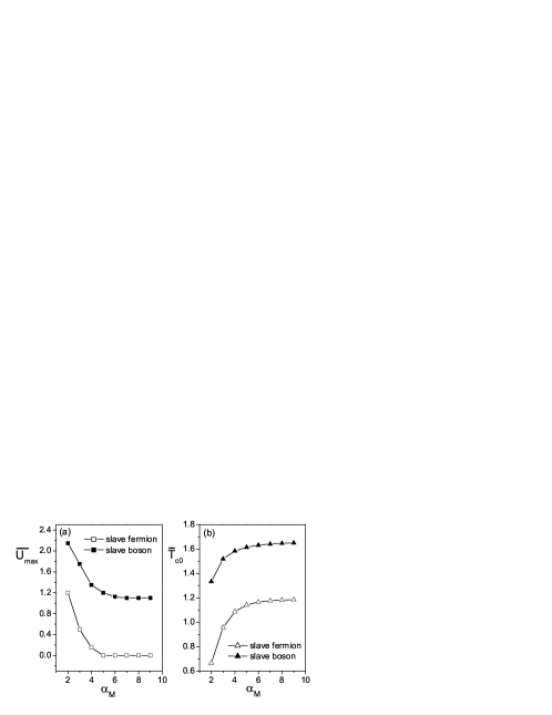
Figure 2: The position of local maximum $\bar{U}_{max}$ (panel (a)) and the critical temperature $\bar{T}_{c0}$ at $\bar{U}=0$ (panel (b)) as a function of the cut-off $\alpha_{M}$ with the average density $n=1$.

We now make a comparison between the phase diagrams in Fig. 1 by these two slave particle approaches. One can see that the $\bar{T}_{c}$ of the slave fermion is always smaller than that of the slave boson. As mentioned in Refs. D and yy , the local maximum in the $\bar{T}_{c}-\bar{U}$ curve is unreasonable. We can see from Fig. 2(a) that, when making a cut-off such as $\alpha_{M}=5$, the position of the local maximum in the slave fermion picture moves to zero, which means the local maximum disappears. However, it seems that the local maximum in the slave boson picture could not be eliminated by merely making a large cut-off. There is still a maximum located around $\bar{U}_{max}=1.1$ even when a large cut-off such as $\alpha_{M}=9$ is made. Moreover, the position of the maximum almost does not depend on the cut-off when $\alpha_{M}>6$. This unsatisfactory feature may come from the approximation of relaxing the constrain of eq. (4), which has less severe effect on the slave fermion than on the slave boson yy . On the other hand, the critical temperature $\bar{T}_{c0}$ at $\bar{U}=0$ should be identical to the Bose-Einstein condensation temperature $\bar{T}_{c}^{ideal}$ of ideal Bose gas, which in the case of three dimensions can be determined by dalfovo ; Kleinert

$$\bar{T}_{c}^{ideal}=\frac{2\pi}{3}\left[\frac{n}{g_{3/2}(0)}\right]^{2/3}$$ (35)

with $n$ being the average particle density and $g_{i}(x)=\sum_{m=1}^{\infty}e^{mx}/m^{i}$. We have $\bar{T}_{c}^{ideal}=1.10$ when $n=1$ note1 . As shown in Fig. 2(b), $\bar{T}_{c0}$ approaches 1.18 and 1.66 for the slave fermion and the slave boson, respectively. Therefore, in this special case of $n=1$, $\bar{T}_{c0}$ of the slave fermion is more appropriate for it is closer to the expected value 1.10. As shown in the phase diagrams, both slave particle approaches yield the critical interaction $\bar{U}_{c}=6$ when $\alpha_{M}=2$, which slightly deviates from the well-known mean field value $\bar{U}_{c}=5.83$. This can be attributed to the mean field approximation of eqs. (32) and (33) and the finite cut-off of $\alpha_{M}$ yy ; D . However, a remedy to the mean field conditions is very difficult yy ; D and, when including more types of slave particles, the calculation of $\bar{T}_{c}$ at very low temperature is very hard too for the divergence and the multi-solutions at $\bar{U}>6$ yy . Hence, when $\alpha_{M}>2$, we actually do not work out $\bar{T}_{c}$ in the very low temperature region in this work note2 .

All the critical temperatures calculated above are concentrated on the commensurate state with fixed integer density (i.e. $n=1$), which is important only to the exact quantum phase transition at $T=0$. We next turn to investigate the $\bar{T}_{c0}$ away from the integer filling and compare them with the critical temperature of ideal Bose gas. In Fig. 3, the dependence of $\bar{T}_{c0}$ on average density $n$ is plotted by both slave particle approaches, and the critical temperature of three-dimensional ideal Bose gas is plotted by eq. (35). We can see that the slave fermion curve is always below the slave boson curve and closer to that of ideal Bose gas. On the other hand, the deviations between both slave particle curves and the ideal gas curve become larger as the density increases. As mentioned above, the multi-occupation of slave particles on one site is allowed in mean field approximation. In the high density region, the multi-occupation may occur more frequently for one should take more types of slave particles into account. This is why the deviations from the ideal gas become large in this region. However, in the slave fermion approach, multi-occupation of the same type of slave fermion is excluded, which makes this approximation less severe than in the slave boson approach and gives a curve closer to that of the ideal gas. One may notice that there is an unsatisfied feature in the slave fermion picture too. The slave fermion curve and the ideal Bose gas curve cross at two different values of the filling, which implies that the slave fermion can not give the correct function dependence of $\bar{T}_{c0}$ on $n$. In the end, we would pay some attention to the mean field nature of our theory. As we know, $\bar{T}_{c0}$ is calculated on base of the mean field approximation and hence applicable to any spatial dimensions. This will lead to the conclusion that the Bose-Einstein condensation occurs in one and two-dimensional ideal Bose gas at finite temperature, which is obviously wrong for the violation of the Hohenberg theorem pitaevskii . However, this is a well known flaw: mean field theory usually breaks down in low dimensions due to the large quantum fluctuation pitaevskii .

Figure 3: The critical temperature $\bar{T}_{c0}$ at $\bar{U}=0$ as a function of average density $n$ with the cut-off $\alpha_{M}=6$. The dashed and dotted lines correspond to the slave boson and slave fermion, respectively. The solid line is the critical temperature of ideal Bose gas in three dimensions.

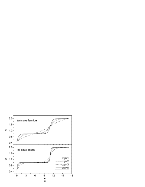
Figure 4: The average particle density $n$ as a function of $\bar{\mu}$ with $\bar{U}=11$ at various temperatures, obtained by the slave fermion (Fig. 4(a)) and slave boson (Fig. 4(b)) approaches. The $\bar{\mu}$ and $\bar{U}$ are the dimensionless chemical potential and on-site interaction, respectively. Six types of slave particles (from $n^{0}$ to $n^{5}$) are taken into account in the calculation. The compressibility can be read out from the slope of the curve.

IV Density and compressibility

The central features of the Mott-insulator at $T=0$ are the integer filling factor $n^{\alpha}=\delta_{\alpha,\alpha^{\prime}}$ and the zero compressibility $\kappa=\partial{n}/\partial{\mu}=0$. At finite temperature, there is no exact Mott-insulating phase because the local filling factor may deviate from an integer and the compressibility $\kappa$ does not equal zero. We will investigate the finite temperature properties of these parameters in this section. In principle, when given the value of $\bar{U}$, one can calculate every type of occupation numbers $n^{\alpha}$ as a function of $\bar{\mu}$ by combining eq. (24) with eq. (32). Then the average particle density $n$, which is a function of $\bar{\mu}$ too, can be obtained according to eq. (33). After depicting the $n-\bar{\mu}$ curve, one can read out the compressibility from the slope of the curve. In Fig. 4, we show the calculated $n-\bar{\mu}$ curves with $\bar{U}=11$ at different temperature in both slave fermion and slave boson pictures. As the figure shows, there are ”steps” on the curves at very low temperature, where the density is very close to an integer and the compressibility is almost equal to zero. It is therefore reasonable to call these regions the ”Mott-insulator” at finite temperature D . We can see that the Mott-insulating regions in both slave particle pictures diminish and disappear gradually as the temperature is increased. However, the quantitative behaviors of them are a little different, i.e., at the same temperature, the compressibility of the slave fermion deviates from zero more greatly than that of the slave boson. This implies that the influence of temperature is greater on the slave fermion than on the slave boson. In Fig. 4, there are only two ”steps” corresponding to $n=1$ and $n=2$. One can obtain the higher ”steps” by including more types of slave particles and working on the larger $\bar{\mu}$. Note that, although the qualitative behavior of this ”step” structure is quite in accord with the zero temperature density profile oosten , the value of the density deep in the superfluid region is unreliable for the invalidity of perturbation theory.

V Superfluid density

As mentioned above, the action near the critical point can be expended in powers of the order parameter $\Phi_{\textbf{0},0}$,

$$S_{E,eff}=\beta\Omega_{0}-G^{-1}(\textbf{0},0)|\Phi_{\textbf{0},0}|^{2}+a_{4}|\Phi_{\textbf{0},0}|^{4}.$$ (36)

If the coefficient $a_{4}$ of fourth order term is positive, the superfluid density $n_{0}$ can be determined by

$$n_{0}=|\langle\Phi_{\textbf{0},0}\rangle|^{2}=\frac{G^{-1}(\textbf{0},0)}{2a_{4}},$$ (37)

which minimizes the action. We calculate the coefficient $a_{4}$ following the steps in Ref. D and show the detailed calculation in Appendix A. The final result is

$$a_{4}= - \frac{{\epsilon_{0}}^{4}}{2L\beta}\sum_{\alpha}\left\{\frac{(\alpha+1)^{2}\beta}{(\mu-{\alpha}U)^{2}}[n^{\alpha}(1{\mp}n^{\alpha})+n^{\alpha+1}(1{\mp}n^{\alpha+1})]+\frac{2(\alpha+1)^{2}}{({\alpha}U-\mu)^{3}}(n^{\alpha+1}-n^{\alpha})\right.$$

$$+ \left.\frac{2(\alpha+1)(\alpha+2)}{(\mu-{\alpha}U)^{2}[(2\alpha+1)U-2\mu]}n^{\alpha}-\frac{2(\alpha+1)(\alpha+2)}{[\mu-(\alpha+1)U]^{2}[(2\alpha+1)U-2\mu]}n^{\alpha+2}\right.$$

$$- \left.\frac{2(\alpha+1)(\alpha+2)U}{(\mu-{\alpha}U)^{2}[\mu-(\alpha+1)U]^{2}}n^{\alpha+1}-\frac{2(\alpha+1)(\alpha+2)\beta}{(\mu-{\alpha}U)[\mu-(\alpha+1)U]}n^{\alpha+1}(1\mp n^{\alpha+1})\right\},$$

where $\mp$ correspond to the slave fermion or the slave boson note and $n^{\alpha}$ is defined in eq. (24). In Fig. 5, we plot the dimensionless $\bar{a}_{4}=L{\beta}a_{4}/zt$ as a function of the chemical potential $\bar{\mu}$ with $\bar{U}=12$ and $zt\beta=4$. We can see that the sign difference in $a_{4}$ (i.e., $\mp$) leads to a very striking result, i.e., $a_{4}$ of the slave boson is always negative. This means the Landau free energy is not minimized but maximized at eq. (37), that is, the mean field theory of the slave boson is not stable and can not give the Landau second order phase transition. The physical reason for this instability may come from the condensation of the slave bosons due to the relaxation of the constraint of one salve boson per site. To see this point more explicitly, we depict in Fig. 6 the dependence of the superfluid density $|\Phi_{\textbf{0},0}|^{2}$ on the chemical potential $\bar{\mu}$ at various temperature. The inset shows the value of $G(\textbf{0},0)/2a_{4}$ as a function of $\bar{\mu}$ in the slave boson picture. We can see that it is opposite to the standard mean field theory at $T=0$ fisher ; Sheshardi , e.g., the ”superfluid density” grows up at the places where are Mott-insulating regions in the zero temperature phase diagram note3 .

Figure 5: The dimensionless fourth-order coefficient $\bar{a}_{4}=L{\beta}a_{4}/zt$ as a function of chemical potential $\bar{\mu}$ by the slave fermion and the slave boson approaches. In the calculation, $\bar{U}=12$, $zt\beta=4$, and four types of slave particles ($n^{0}$, $n^{1}$, $n^{2}$, and $n^{3}$) are taken into account.

In the slave fermion approach, $a_{4}$ is positive definitely. Then the Landau second order phase transition theory may be safely applied. As shown in the Fig. 6, the superfluid regions are consistent with those in the zero temperature phase diagram, and become small and disappear gradually when the temperature is increased. It is notable that the perturbation theory used here is valid only near the critical point. Thus the value of the superfluid density far away from the critical point may be incorrect. The accurate value can be obtained by means of the Bogoliubov theory dalfovo , but this is beyond the scope of this paper. Because only four types of slave fermions are considered, the superfluid phase in the larger $\bar{\mu}$ region, which corresponds to the higher filling factor, could not be obtained in our calculation.

Figure 6: Superfluid density $|\Phi_{\textbf{0},0}|^{2}$ as a function of chemical potential $\bar{\mu}$ with $\bar{U}=12$ at different temperature. Four types of slave particles ($n^{0}$, $n^{1}$, $n^{2}$, and $n^{3}$) are taken into account. The solid, dotted, dashed-dotted-dotted, and dashed lines are obtained by the slave fermion approach and correspond to $zt\beta=$ 7, 4, 2.5, and 1.8, respectively. Inset shows the value of $G(\textbf{0},0)/2a_{4}$ in the slave boson picture with $zt\beta=7$, which should not be regarded as the superfluid density because the $a_{4}$ is always negative.

VI The excitation spectrum

The excitation spectrum of the quasiparticle and quasihole can be determined by the pole of the Green’s function, that is, by the equation $G^{-1}(\textbf{k},\omega)=0$. From eq. (28), we have

$$\sum_{\alpha=0}(\alpha+1)\frac{n^{\alpha+1}-n^{\alpha}}{\omega+\mu-{\alpha}U}=\frac{1}{\epsilon_{\textbf{k}}}.$$ (39)

It is easy to show that both slave particle approaches give the same excitation spectrum at $T=0$ for $n^{\alpha}=\delta_{\alpha,\alpha^{\prime}}$ with $\alpha^{\prime}$ being an integer filling factor. At nonzero temperature, one should take more than one type of slave particle into account and eq. (39) will have more than two solutions D . In the case of low density $n=1$, it is reasonable to take only three types of slave particles ($n^{0}$, $n^{1}$ and $n^{2}$) into account, that is, only the processes in which the occupation of a site changes among $n^{0}$, $n^{1}$ and $n^{2}$ are considered D . By this approximation, we can obtain two low-lying excitation spectra analytically,

$$\begin{split}\omega_{\textbf{k}}^{\pm}+\mu&=\frac{U}{2}+\frac{1}{2}\epsilon_{\textbf{k}}(2n^{2}-n^{1}-n^{0})\\ &\pm\frac{1}{2}\sqrt{U^{2}+2(n^{0}-3n^{1}+2n^{2})U\epsilon_{\textbf{k}}+(n^{0}+n^{1}-2n^{2})^{2}\epsilon_{\textbf{k}}^{2}}.\end{split}$$ (40)

Figure 7: The excitation energies $(\omega+\mu)/zt$ as a function of the dimensionless on-site interactions $\bar{U}$ at $\textbf{k}=0$ for various temperatures. Panel (a) and (b) are obtained by the slave fermion and the slave boson approaches, respectively. The inset in panel (a) shows the energy gap between quasiparticle and quasihole excitations. The average density is set to be $n=N/L=1$ and three types of slave particles ($n^{0}$, $n^{1}$, and $n^{2}$) are taken into account.

In Fig.7, we show the excitation energies $(\omega+\mu)/zt$ as a function of $\bar{U}$ at $\textbf{k}=0$ for various temperatures. We can see that the tip of the lobe, where the gap for quasiparticle-quasihole excitation disappears, moves to the small $\bar{U}$ region as the temperature increases. This picture is qualitatively consistent with the superfluid-normal phase diagram obtained in Sect. III. Another feature of this figure is that the energy gap for quasiparticle-quasihole excitation is enlarged as the temperature or the interaction $\bar{U}$ is increased. Recently, Konabe et al. have obtained the same result by a standard basis operator method Konabe . When comparing panel (a) with panel (b), we can see that, at the same temperature, the lobe by the slave fermion evolves away from zero temperature lobe more greatly than that by the slave boson, from which we can conclude again that the influence of temperature on the slave fermion is larger than that on the slave boson. Note that, except the point of $\bar{U}=0$, the quasiparticle and quasihole branches do not meet at finite temperature, e.g., the dotted line in Panel (a) and dashed-dotted-dotted line in Panel (b) (the gap is very small). This may be due to the finite cut-off approximation and can be remedied by including more types of slave particles. In addition, the two branches of spectrum always meet at (0,0) at high temperature. The reason is that, when the temperature is high enough, one would have $n^{0}=n^{1}=n^{2}=0.333$ at $\bar{U}=0$ and then the right hand side of eq. (40) would always equal zero. In all, eq. (40) is valid only at very low temperature and near the Mott-insulator, where the approximation of $\alpha_{M}=2$ is justified.

By using the slave fermion approach, we show, in Fig. 8, the dispersion relation of a two-dimensional atomic gas in a square optical lattice at various temperatures. The behavior of the dispersion curves at zero temperature, marked by the solid lines, is qualitatively similar to that obtained by Sengupta et al. seng using a strong-coupling expansion approach. At finite temperature, we can see that, in the different regions of the Brillouin zone, the influence of the temperature on the gap for quaiparticle-quasihole excitation is different. In the region between $(\pi,0)$ and $(\pi/2,\pi/2)$, the gap increases as the temperature is increased. However, in the region from $(\pi/2,\pi/2)$ to $(\pi,0)$, the gap diminishes when we increase the temperature. One can see that the temperature affects the excitation spectrum greatly at the points $(0,0)$ and $(\pi,\pi)$, but at other points such as $(\pi,0)$ and $(\pi/2,\pi/2)$ the influence of temperature is very small.

Figure 8: The dispersion relation $(\omega+\mu)/zt$ of a two-dimensional atomic gas in a square optical lattice at various temperatures. The results are obtained by the slave fermion approach and with $\bar{U}=7.5$. The solid, dotted, dashed-dotted-dotted, and dashed lines correspond to $zt\beta=$ infinity, 2, 1, and 0.5, respectively.

VII Conclusions

The finite temperature properties of the Bose-Hubbard model were investigated by both slave boson and slave fermion approaches. Many physical quantities were calculated in the mean field level and we found in general there are no qualitatively differences either by using the slave boson or slave fermion approaches. However, when studying the stability of the mean field state, we found that in contrast to slave fermion approach, the slave boson mean field state is not stable. The mean field phase diagram of superfluid-normal transition was obtained by making a relative large $\alpha$ cut-off (e.g. $\alpha_{M}=6$), and the effect of the finite types of slave particles was estimated. The unreasonable local maximum in the phase diagram can be eliminated in the slave fermion approach by increasing the cut-off, but it can not be eliminated in the slave boson approach. In the low density region, the critical temperature at $\bar{U}=0$ by our mean field approaches is quite close to the Bose-Einstein condensation temperature of ideal Bose gas in three dimensions. The particle density was derived and depicted as a function of chemical potential $\bar{\mu}$. The ”Mott-insulating” phase at finite temperature, where the filling factor is very close to an integer, was identified and how it evolves as the temperature increases was demonstrated. The superfluid density was calculated and plotted as a function of chemical potential $\bar{\mu}$. We showed that the slave boson approach could not give a correct superfluid density because the coefficient $a_{4}$ in the Landau free energy expansion is always negative. The low-lying excitation spectra were obtained analytically by taking three types of slave fermions ($n^{0}$, $n^{1}$ and $n^{2}$) into account, and were plotted as a function of $\bar{U}$ and in the k space at different temperatures. It was shown that, in the different region of the Brillouin zone, the influence of the temperature on the quasiparticle-quasihole gap is different.

Appendix A the coefficient of fourth order term

In this section we turn to calculate the coefficient $a_{4}$ of fourth order term by both slave fermion and slave boson approaches, following the steps in Ref. D . We are only interested in the $\Phi_{00}$ terms and can write the partition function of eq. (14) as

$$Z={\int}D\Phi_{00}^{*}D\Phi_{00}D\bar{a}_{\alpha}Da_{\alpha}{e^{-S}},$$

$$S=iL\beta\lambda+\epsilon_{0}|\Phi_{00}|^{2}+\sum_{\alpha\beta}\sum_{\textbf{k},n}\bar{a}_{\alpha,{\textbf{k}n}}M^{\alpha\beta}a_{\beta,{\textbf{k}n}},$$ (1)

where $\bar{a}_{\alpha,{\textbf{k}n}}$ and $a_{\alpha,{\textbf{k}n}}$ are the Grassmann variables in the slave fermion picture and the ordinary complex numbers in slave boson picture, $M$ is a matrix:

$$\begin{pmatrix}\chi_{0}&A_{0}&&&&\\ B_{0}&\chi_{1}&A_{1}&&&\\ &B_{1}&\chi_{2}&A_{2}&&\\ &&B_{2}&\chi_{3}&A_{3}\\ &&&&...&\end{pmatrix}\quad$$

with

$$A_{\alpha} = -\frac{\sqrt{\alpha+1}}{\sqrt{L\beta}}\epsilon_{0}\Phi_{00}^{*},$$

$$B_{\alpha} = -\frac{\sqrt{\alpha+1}}{\sqrt{L\beta}}\epsilon_{0}\Phi_{00},$$

$$\chi_{\alpha} = -i\omega_{n}+c(\alpha),$$

in which $c(\alpha)$ is defined in eq. (15). We then integrate the slave particle fields out of the partition function and obtain the effective action $S_{eff}^{\prime}$,

$$Z = \int D\Phi_{00}^{*}D\Phi_{00}e^{-S_{eff}^{\prime}}$$

$$= \int D\Phi_{00}^{*}D\Phi_{00}\exp\left\{-\left(iL\beta\lambda+\epsilon_{0}|\Phi_{00}|^{2}\mp\sum_{\textbf{k},n}\ln{[\det\beta{M}]}\right)\right\}$$

$$S_{eff}^{\prime} = iL\beta\lambda+\epsilon_{0}|\Phi_{00}|^{2}\mp\sum_{\textbf{k},n}\ln{[\det\beta{M}]},$$ (2)

where $\mp$ correspond to slave fermion or slave boson. The determinant of $\beta{M}$ can be written as

$$\det\beta{M} = \left(\prod_{\alpha}\beta\chi_{\alpha}\right)\left[1-\sum_{\alpha}\frac{\epsilon_{0}^{2}}{L\beta}\frac{(\alpha+1)}{\chi_{\alpha}\chi_{\alpha+1}}|\Phi_{00}|^{2}\right.$$

$$\left.+\sum_{\alpha}\sum_{|\alpha-\beta|\geq 2}\frac{\epsilon_{0}^{4}}{(L\beta)^{2}}\frac{(\alpha+1)(\beta+1)}{\chi_{\alpha}\chi_{\alpha+1}\chi_{\beta}\chi_{\beta+1}}|\Phi_{00}|^{4}+\cdots\right].$$

In the case of small $\Phi_{00}$, $\ln{[\det\beta{M}]}$ can be expanded by using

$$\ln(1-A|\Phi_{00}|^{2}+B|\Phi_{00}|^{4})=-A|\Phi_{00}|^{2}+\frac{1}{4}(-2A^{2}+4B)|\Phi_{00}|^{4}+O(|\Phi_{00}|^{5}).$$

Then the effective action up to fourth order in $\Phi_{00}$ can be given by

$$S_{eff}^{\prime} = iL\beta\lambda\mp\sum_{n}L\ln\left(\prod_{\alpha}\beta\chi_{\alpha}\right)+\left[\epsilon_{0}\pm\frac{\epsilon_{0}^{2}}{\beta}\sum_{n}\sum_{\alpha}\frac{(\alpha+1)}{\chi_{\alpha}\chi_{\alpha+1}}\right]|\Phi_{00}|^{2}$$

$$\mp \frac{L}{4}\left(\frac{\epsilon_{0}}{\sqrt{L\beta}}\right)^{4}\sum_{n}\left[-2\left(\sum_{\alpha}\frac{(\alpha+1)}{\chi_{\alpha}\chi_{\alpha+1}}\right)^{2}+\sum_{\alpha}\sum_{|\alpha-\beta|\geq 2}\frac{4(\alpha+1)(\beta+1)}{\chi_{\alpha}\chi_{\alpha+1}\chi_{\beta}\chi_{\beta+1}}\right]|\Phi_{00}|^{4},$$

where the summation over k leads to the number $L$ of lattice sites. The coefficient $a_{2}$ of the second-order term $|\Phi_{00}|^{2}$ can be read out directly from eq. (A),

$$a_{2} = \epsilon_{0}\pm\frac{\epsilon_{0}^{2}}{\beta}\sum_{n}\sum_{\alpha}\frac{(\alpha+1)}{\chi_{\alpha}\chi_{\alpha+1}}$$ (4)

$$= \epsilon_{0}-{\epsilon_{0}}^{2}\sum_{\alpha}(\alpha+1)\frac{n^{\alpha}-n^{\alpha+1}}{-\mu+{\alpha}U}=-G^{-1}(0,0),$$

where $\pm$ corresponds to slave fermion or slave boson. We can see that both slave fermion and slave boson approaches reduce to the same result $-G^{-1}(0,0)$. The coefficient $a_{4}$ of the fourth-order term $|\Phi_{00}|^{4}$ can be rewritten as

$$a_{4}=\pm\frac{L}{2}\left(\frac{\epsilon_{0}}{\sqrt{L\beta}}\right)^{4}\sum_{n}\sum_{\alpha}\left[\frac{(\alpha+1)^{2}}{\chi_{\alpha}\chi_{\alpha}\chi_{\alpha+1}\chi_{\alpha+1}}+\frac{2(\alpha+1)(\alpha+2)}{\chi_{\alpha}\chi_{\alpha+1}\chi_{\alpha+1}\chi_{\alpha+2}}\right],$$ (5)

where $\pm$ corresponds to slave fermion or slave boson. Typically, we calculate the first term

$$\pm\frac{1}{\beta}\sum_{n}\left[\frac{(\alpha+1)^{2}}{\chi_{\alpha}\chi_{\alpha}\chi_{\alpha+1}\chi_{\alpha+1}}\right]=\pm\frac{1}{\beta}\sum_{n}\frac{(\alpha+1)}{\left[i\omega_{n}-c(\alpha)\right]^{2}}\frac{(\alpha+1)}{\left[i\omega_{n}-c(\alpha+1)\right]^{2}}.$$ (6)

The frequency summations in this term can be performed by using

$$\pm\frac{1}{\beta}\sum_{n}f(i\omega_{n})={\rm Res}\left[f(z)\frac{1}{e^{{\beta}z}\pm 1}\right]_{c(\alpha)}+{\rm Res}\left[f(z)\frac{1}{e^{{\beta}z}\pm 1}\right]_{c(\alpha+1)}.$$ (7)

Res$\left[F(z)\right]_{c(\alpha)}$ denotes the residue of $F(z)$ at the pole $c(\alpha)$, and for the $m$-th order pole, can be determined by

$${\rm Res}\left[F(z)\right]_{c(\alpha)}=\lim_{z\rightarrow{c(\alpha)}}\frac{1}{(m-1)!}{\frac{d^{m-1}}{dz^{m-1}}\left[(z-c(\alpha))^{m}F(z)\right]}.$$ (8)

By using this equation, the value of eq. (6) can be evaluated, which is

$$\pm\frac{1}{\beta}\sum_{n}\left[\frac{(\alpha+1)^{2}}{\chi_{\alpha}\chi_{\alpha}\chi_{\alpha+1}\chi_{\alpha+1}}\right]= - \frac{(\alpha+1)^{2}\beta}{(\mu-{\alpha}U)^{2}}[n^{\alpha}(1{\mp}n^{\alpha})+n^{\alpha+1}(1{\mp}n^{\alpha+1})]$$ (9)

$$- \frac{2(\alpha+1)^{2}}{({\alpha}U-\mu)^{3}}(n^{\alpha+1}-n^{\alpha}).$$

After calculating the second term in eq. (5) in the same way, we can obtain the final expression of $a_{4}$ as shown in eq. (V). In the Mott-insulating region at $T=0$, we have $n^{\alpha}=\delta_{\alpha,g}$ with $g$ being the average density. For the slave fermion, the sign in eq. (V) is minus and then $a_{4}$ is reduced to

$$a_{4}= - \frac{{\epsilon_{0}}^{4}}{L\beta}\left\{\frac{g^{2}}{[(g-1)U-\mu]^{3}}+\frac{(g+1)^{2}}{(\mu-gU)^{3}}\right.$$ (10)

$$- \left.\frac{(g+1)(g+2)}{(\mu-gU)^{2}[2\mu-(2g+1)U]}-\frac{g(g-1)}{[\mu-(g-1)U]^{2}[(2g-3)U-2\mu]}\right.$$

$$- \left.\frac{g(g+1)U}{[(g-1)U-\mu]^{2}[\mu-gU]^{2}}\right\},$$

which is exactly the same as the results in Ref. oosten and Ref. Konabe . However, for the slave boson, the sign in eq. (V) is plus and the result is quite different note . Furthermore, as we have shown in Sec. V, $a_{4}$ is always non-positive, which leads to the instability of the slave boson mean field state.

References

• (1) I. Bloch, Physics World, 17, 25-29 (2004).
• (2) C. Orzel, A. K. Tuchman, M. L. Fenselau, M. Yasuda, and M. A. Kasevich Science 291 2386 (2001).
• (3) M. Greiner, O. Mandel, T. Esslinger, T. W. HΓ€nsch, and I. Bloch, Nature (London) 415, 39 (2002).
• (4) D. Jaksch, C. Bruder, J. I. Cirac, C. W. Gardiner and P. Zoller, Phys. Rev. Lett. 81, 3108 (1998).
• (5) M. P. A. Fisher, P. B. Weichman, G. Grinstein, and D. S. Fisher, Phys. Rev. B 40, 546 (1989).
• (6) J. K. Freericks and H. Monien, Europhys. Lett. 26, 545 (1994).
• (7) J. K. Freericks and H. Monien, Phys. Rev. B 53, 2691 (1996).
• (8) N. Elstner and H. Monien, Phys. Rev. B 59, 12184 (1999).
• (9) K. Sengupta and N. Dupuis, Phys. Rev. A 71, 033629 (2005).
• (10) W. Krauth, M. Caffarel, and J.-P. Bouchaud, Phys. Rev. B 45, 3137 (1992).
• (11) D. S. Rokhsar and B. G. Kotliar, Phys. Rev. B 44, 10328 (1991).
• (12) C. Schroll, F. Marquardt, and C. Bruder, Phys. Rev. A 70, 053609 (2004).
• (13) G. G. Batrouni, V. Rousseau, R. T. Scalettar, M. Rigol, A. Muramatsu, P. J. H. Denteneer, and M. Troyer, Phys. Rev. Lett. 89, 117203 (2002); G. G. Batrouni, R. T. Scalettar, and G. T. Zimanyi, Phys. Rev. Lett. 65, 1765 (1990).
• (14) S. Wessel, F. Alet, M. Troyer, and G. G. Batrouni, Phys. Rev. A 70, 053615 (2004).
• (15) D. van Oosten, P. van der Straten, and H. T. C. Stoof, Phys. Rev. A 63, 053601 (2001).
• (16) K. Sheshardi et al., Europhys. Lett. 22, 257 (1993);
• (17) D. B. M. Dickerscheid, D. van Oosten, P. J. H. Denteneer, and H. T. C. Stoof, Phys. Rev. A 68, 043623 (2003).
• (18) P. Buonsante and A. Vezzani, Phys. Rev. A 70, 033608 (2004);
• (19) S. Konabe, T. Nikuni, M. Nakamura, cond-mat/0407229.
• (20) A. P. Kampf and G. T. Zimanyi, Phys. Rev. B 47, 279 (1993); L. I. Plimak, M. K. Olsen, and M. Fleischhauer, Phys. Rev. A 70, 013611 (2004). D. van Oosten, P. van der Straten, and H. T. C. Stoof, Phys. Rev. A 67, 033606 (2003).
• (21) Yue Yu and S. T. Chui, Phys. Rev. A 71, 033608 (2005).
• (22) G. Kotliar and A. E. Ruckenstein, Phys. Rev. Lett. 57, 1362 (1986); P. Coleman, Phys. Rev. B 29, 3035 (1984).
• (23) K. Ziegler, Europhys. Lett. 23, 463 (1993); K. Ziegler and A. Shukla, Phys. Rev. A 56, 1438(1997); K. Ziegler Phys. Rev. A 62, 023611 (2000).
• (24) R. Fresard, cond-mat/9405053.
• (25) We observed several errors in eq. (A9) of Ref. D in computing the coefficient $a_{4}$. The most obvious and important one is that they took a wrong ’minus’ in the first, third, fifth, ninth, and twelfth terms.
• (26) F. Dalfovo et al., Rev. Mod. Phys. 71, 463 (1999).
• (27) Jinbin Li, Yue Yu and Qian Niu, cond-mat/0311012.
• (28) J. W. Negele and H. Orland, Quantum Many-Particle Systems (Addison-Wesley, Redwood City, 1988).
• (29) H. T. C. Stoof, cond-mat/9910441.
• (30) P. A. Lee, in High Temperature Superconductivity, Proc. Los Alamos Symposium, edited by K. S. Bedell, D. Coffey, D. E. Meltzer, D. Pines, and J. R. Schrieffer (Addison-Wesley, Redwood City, CA, 1989).
• (31) H. Kleinert, S. Schmidt, and A. Pelster, Phys. Rev. Lett. 93, 160402 (2004).
• (32) In the case of $n=1$, $\bar{T}_{c}^{ideal}=2.61^{-2/3}\times 4\pi/6\approx 1.104$. Note that the value provided in endnote [15] of Ref. yy is slightly wrong.
• (33) One can find a calculation with $\alpha_{M}=3$ in Ref. yy . The calculation with $\alpha_{M}>3$ and whether there exists a reentrant behavior would be interesting topics for a further work.
• (34) L. Pitaevskii and S. Stringari, Bose-Einstein Condensation (Oxford University Press, Oxford, 2003).
• (35) The true superfluid density of slave boson can be obtained by including the sixth order term, but this would predict a first order superfluid/normal phase transition at some positive value of $a_{2}$.