Estimate of the free energy difference in mechanical systems from work fluctuations: experiments and models

Abstract

The work fluctuations of an oscillator in contact with a heat reservoir and driven out of equilibrium by an external force are studied experimentally. The oscillator dynamics is modeled by a Langevin equation. We find both experimentally and theoretically that, if the driving force does not change the equilibrium properties of the thermal fluctuations of this mechanical system, the free energy difference $\Delta F$ between two equilibrium states can be exactly computed using the Jarzynski equality (JE) and the Crooks relation (CR) [1, 2, 3], independently of the time scale and amplitude of the driving force. The applicability limits for the JE and CR at very large driving forces are discussed. Finally, when the work fluctuations are Gaussian, we propose an alternative method to compute $\Delta F$ which can be safely applied, even in cases where the JE and CR might not hold. The results of this paper are useful to compute $\Delta F$ in complex systems such as the biological ones.

1 Introduction

A precise characterization of the dynamics of mesoscopic and macroscopic systems is a very important problem for applications in nanotechnologies and biophysics. While fluctuations always play a negligible role in large systems, their influence may become extremely important in small systems driven out of equilibrium. Such is the case for nanoengines and biological processes, where the characteristic amount of energy transferred by fluctuations can be of the same order as that which operates the device. In these small out of equilibrium systems, dominated by thermal fluctuations, a precise estimation of the free energy difference $\Delta F$ between two equilibrium states $A$ and $B$ is extremely useful to increase our knowledge of the underlying physical processes which control their dynamical behaviour. It is well known that $\Delta F$ can be estimated by perturbing a system with an external parameter $\lambda$ and by measuring the work $W$ done to drive the system from $A$ to $B$. When thermal fluctuations cannot be neglected $W$ is a strongly fluctuating quantity and $\Delta F$ may in principle be computed using the Jarzynski equality (JE) [1] and the Crooks relation (CR) [2] (see section 2 for their definition). Indeed the JE and CR take advantage of these work fluctuations and relate the $\Delta F$ to the probability distribution function (pdf) of the work performed on the system to drive it from $A$ to $B$ along any path $\gamma$ ( either reversible or irreversible) in the system parameter space. Numerous derivations of the JE and CR have been produced [6, 7, 8, 9, 10] and JE and CR have been used in order to estimate the free energy of a stretched DNA molecule [5, 4]. However the derivation of JE in the case of strongly irreversible systems has been criticized in ref.[11]. For this reason in a recent letter [12], we have experimentally checked JE and CR on a very simple and controlled device in order to safely use these two relations in more complex cases as the biological and chemical ones, where it is much more difficult (almost impossible) to verify the results with other methods. Our system is a mechanical oscillator, in contact with a heat bath, which is driven out of equilibrium, between two equilibrium states $A$ and $B$, by a small external force. In ref.[12] we have shown that the JE and CR are experimentally accessible and valid for all the values of the different control parameters. However one may wonder whether the driving force’s switching rate and its amplitude were fast and large enough. Therefore in this paper we extend the measurements of ref.[12] till the limits of the experimental set up. We find that even in these extreme cases the $\Delta F$ is correctly estimated by JE and CR. We also observe that these experimental results can be exactly derived from a Langevin equation if one takes into account that, experimentally, the properties of the thermal noise are not changed by the external driving force. These conditions are close to those pointed out in Ref. [11] for the validity of the JE, thus they do not fully alight the theoretical debate. However the fact of having driven the system at large driving amplitudes and the study of the corresponding Langevin dynamics allow us to clearly understand the experimental limits of applicability of the JE and CR. Independently on the theoretical problems that the derivation of JE may rise, these limits are of statistical nature and they strongly reduce the possibility of using JE and CR when the driving energy is much larger than the thermal energy. As a consequence these intrinsic statistical limits make the experimental test of the criticisms arisen in Ref. [11] very difficult almost impossible. However, when the fluctuations of $W$ are Gaussian we propose here an alternative method to compute $\Delta F$, which can be useful even in cases where the JE and the CR could not hold.

The paper is organized as follows. In section 2 we recall the JE and CR and we discuss the Gaussian case. In section 3 we describe the experimental setup and in section 4 the experimental results. In section 5 we show that for a Langevin equation the JE gives the exact value of the free energy difference for any path. In section 6 we discuss the limits of applicability of JE and CR and we conclude.

2 The Jarzynski equality and the Crooks relation

In 1997 [1] Jarzynski derived an equality which relates the free energy difference of a system in contact with a heat reservoir to the pdf of the work performed on the system to drive it from $A$ to $B$ along any path $\gamma$ in the system parameter space.

2.1 The Jarzynski equality

Specifically, when $\lambda$ is varied from time $t=0$ to $t=t_{s}$, Jarzynski defines for one realization of the “switching process” from $A$ to $B$ the work performed on the system as

$$W=\int_{0}^{t_{s}}\dot{\lambda}\,\frac{\partial H_{\lambda}[z(t)]}{\partial\lambda}\,\mathrm{d}t,$$ (1)

where $z$ denotes the phase-space point of the system and $H_{\lambda}$ its $\lambda$-parametrized Hamiltonian (see also [13] and section 2.4). One can consider an ensemble of realizations of this “switching process” with initial conditions all starting in the same initial equilibrium state. Then $W$ may be computed for each trajectory in the ensemble. The JE states that [1]

$$\Delta F=-\frac{1}{\beta}\ln\langle\exp{[-\beta W]}\rangle,$$ (2)

where $\langle{\cdot}\rangle$ denotes the ensemble average, $\beta^{-1}=k_{B}T$ with $k_{B}$ the Boltzmann constant and $T$ the temperature. In other words $\langle\exp{[-\beta W_{\mathrm{diss}}]}\rangle=1$, since we can always write $W=\Delta F+W_{\mathrm{diss}}$ where $W_{\mathrm{diss}}$ is the dissipated work. Thus it is easy to see that there must exist some microscopic trajectories such that $W_{\textrm{diss}}\leq 0$. Moreover, the inequality $\langle\exp{x}\rangle\geq\exp{\langle x\rangle}$ allows us to recover the second principle, namely $\langle W_{\textrm{diss}}\rangle\geq 0$, i.e. $\langle W\rangle\geq\Delta F$. From an experimental point of view the JE is quite useful because there is no restriction on the choice of the path $\gamma$ and it overcomes the above mentioned experimental difficulties.

As we have already mentioned in the introduction, many proofs of the JE have been done. The simplest way to understand JE is to consider the perturbation theory [13, 14]. This kind of approach has been used by Landau [13] but he considered only Gaussian distributions and he stopped the development to the second order. This technique can be generalized to get JE. Therefore we follow ref.[13] and we write the energy $H_{B}(p,q)$ of the system in contact with a heath bath at temperature $T$ as:

$$H_{B}(p,q)=H_{A}(p,q)+V(p,q,\lambda(t_{s}))$$ (3)

where $V$ is the energy introduced by the external driving $\lambda$ such that $V(p,q,\lambda(0))=0$. By definition the $\Delta F$ is given by

$$F_{B}=F_{A}-\beta^{-1}\ln\int\rho_{A}\ \exp{[-\beta V]}d\Gamma$$ (4)

where $\rho_{A}(p,q)=\exp{[\beta(F_{A}-H_{A}(p,q))]}$ is the equilibrium Gibbs distribution in $A$, that is the unperturbed state. Therefore

$$F_{B}=F_{A}-\beta^{-1}\ln<\exp{[-\beta V]}>.$$ (5)

As ${dH\over dt}={\partial H\over\partial t}$ [15] and $H$ depends explicitly on time only by mean of $\lambda$ then

$$V=H_{B}-H_{A}=\int_{0}^{t_{s}}{dH\over dt}dt=\int_{0}^{t_{s}}{\partial H\over\partial\lambda}{d\lambda\over dt}dt.$$ (6)

Comparing eq.6 to eq.1 we see that $V=W$ and eq.5 is equivalent to eq.2.

2.2 The Crooks relation

In our experiment we can also check the CR which is somehow related to the JE and which gives useful and complementary information on the dissipated work. Crooks considers the forward work $W_{\mathrm{f}}$ to drive the system from $A$ to $B$ and the backward work $W_{\mathrm{b}}$ to drive it from $B$ to $A$. If the work pdfs during the forward and backward processes are $\mathrm{P}_{\mathrm{f}}(W)$ and $\mathrm{P}_{\mathrm{b}}(W)$, one has [2, 3]

$$\frac{\mathrm{P}_{\mathrm{f}}(W)}{\mathrm{P}_{\mathrm{b}}(-W)}=\exp{(\beta[W-\Delta F])}=\exp{[\beta W_{\mathrm{diss}}]}.$$ (7)

A simple calculation from Eq. (7) leads to Eq. (2). However, from an experimental point of view this relation is extremely useful because one immediately sees that the crossing point of the two pdfs, that is the point where $\mathrm{P}_{\mathrm{f}}(W)=\mathrm{P}_{\mathrm{b}}(-W)$, is precisely $\Delta F$. Thus one has another mean to check the computed free energy by looking at the pdfs crossing point $W_{\mathrm{\times}}$.

2.3 The Gaussian case

Let us examine in some detail the Gaussian case, that is $\mathrm{P}(W)\propto\exp{\Bigl{(}-\frac{[W-\langle W\rangle]^{2}}{2\sigma_{W}^{2}}}\Bigr{)}$. In this case the JE leads to

$$\Delta F=\langle W\rangle-\frac{\beta\sigma_{W}^{2}}{2},$$ (8)

i.e. $\langle W_{\textrm{diss}}\rangle=\frac{\beta\sigma_{W}^{2}}{2}>0$. It is interesting to notice that Landau [13] derived eq.8, which can also be viewed as a consequence of the linear response theory as it has been shown by Hermans [16].

It is easy to see from Eq. (7) that if $\mathrm{P}_{\mathrm{f}}(W)$ and $\mathrm{P}_{\mathrm{b}}(-W)$ are Gaussian, then

$$\Delta F=\frac{\langle W\rangle_{\mathrm{f}}-\langle W\rangle_{\mathrm{b}}}{2},$$ (9)

and

$$\qquad\beta\sigma_{W}^{2}=\langle W\rangle_{\mathrm{f}}+\langle W\rangle_{\mathrm{b}}=2\,\langle W_{\mathrm{diss}}\rangle.$$ (10)

Thus in the case of Gaussian statistics $\Delta F$ and $W_{\mathrm{diss}}$ can be computed by using just the mean values and the variance of the work $W$.

2.4 The classical work and the $\Delta F$ computed by the JE

Before describing the experiment, we want to discuss several important points. The first is the definition of the work given in Eq. (1), which is not the classical one. Let us consider, for example, that $\lambda$ is a mechanical torque $M$ applied to a mechanical system $\Xi$, and $-\partial H_{\lambda}/\partial\lambda$ the associated angular displacement $\theta$. Then, from Eq. (1), one has

$$W=-\int_{0}^{t_{s}}\dot{M}\theta\,\mathrm{d}t=-\Bigl{[}M\theta\Bigr{]}_{0}^{t_{s}}-W^{\mathrm{cl}},$$ (11)

where

$$W^{\mathrm{cl}}=-\int_{0}^{t_{s}}M\dot{\theta}\,\mathrm{d}t$$ (12)

is the classical work (we define the classical work with minus sign to respect the standard convention of thermodynamics). Thus $W$ and $W^{\mathrm{cl}}$ are related but they are not exactly the same and we will show that this makes an important difference in the fluctuations of these two quantities. This difference between the $W$ and $W^{cl}$, has been already pointed out in ref.[17].

The second important point that we want to discuss concerns the $\Delta F$ computed by the JE in the case of a driven system, composed by $\Xi$ plus the external driving. The total free energy difference is

$$\Delta F=\Delta F_{0}-\Bigl{[}M\theta\Bigr{]}_{A}^{B}=\Delta F_{0}-\Phi,$$ (13)

where $\Delta F_{0}$ is the free energy of $\Xi$ and $\Phi=\Bigl{[}M\theta\Bigr{]}_{A}^{B}$ the energy difference of the forcing. The JE computes the $\Delta F$ of the driven system and not that of the system alone which is $\Delta F_{0}$. This is an important observation in view of all applications where an external parameter is added to $\Xi$ in order to measure $\Delta F_{0}$ [5]. Finally we point out that, in an isothermal process, $\Delta F_{0}$ can be easily computed, without using the JE and the CR, if $W^{\mathrm{cl}}$ is Gaussian distributed with variance $\sigma_{W^{\mathrm{cl}}}^{2}$. (We make the reasonable assumption that forward and backward work variances are equal.) Indeed the crossing point $W_{\times}^{\mathrm{cl}}$ of the two Gaussian pdfs $\mathrm{P}_{\mathrm{f}}(W^{\mathrm{cl}})$ and $\mathrm{P}_{\mathrm{b}}(-W^{\mathrm{cl}})$ is

$$W_{\times}^{\mathrm{cl}}=\frac{\langle W^{\mathrm{cl}}\rangle_{\mathrm{f}}-\langle W^{\mathrm{cl}}\rangle_{\mathrm{b}}}{2},$$ (14)

which by definition is just $-\Delta F_{0}$, i.e. $W_{\times}^{\mathrm{cl}}=-\Delta F_{0}$. Furthermore the dissipated work can be obtained from

$$\langle W_{\mathrm{diss}}\rangle\ =-{\langle W^{\mathrm{cl}}\rangle_{\mathrm{f}}+\langle W^{\mathrm{cl}}\rangle_{\mathrm{b}}\over 2},$$ (15)

by definition. It should be noted that the equality $2\,\langle W_{\mathrm{diss}}\rangle=\beta\sigma_{W^{\mathrm{cl}}}^{2}$ does not hold in the case of the classical work.

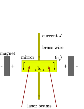
Figure 1: Schematic drawing of the oscillator

(i)                                (ii)                                (iii)

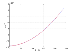
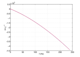
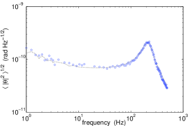
Figure 2: FDT check in oil. i) Real part $1/\chi$. ii) Imaginary part of $1/\chi$. iii) Noise spectrum the circles $(\circ)$ correspond to the direct measurement of the noise and the dashed curve is $\sqrt{\langle{|\hat{\theta}|}^{2}\rangle}$ computed by inserting the measured response function $\chi$ in the FDT, Eq. (18)

3 Experimental setup

3.1 The torsion pendulum

To study the JE and the CR we measure the out-of-equilibrium fluctuations of a macroscopic mechanical torsion pendulum made of a brass wire, whose damping is given either by the viscoelasticity of the torsion wire or by the viscosity of a surrounding fluid. This system is enclosed in a cell which can be filled with a viscous fluid, which acts as a heat bath. A brass wire of length $10\textrm{ mm}$, width $0.75\textrm{ mm}$, thickness $50\textrm{ }\mu\textrm{m}$, mass $5.91\times 10^{-3}\textrm{ g}$, is clamped at both ends, hence its elastic torsional stiffness is $C=7.50\times 10^{-4}\textrm{ N\,m}\mathrm{\,rad^{-1}}$. A small mirror of effective mass $4.02\times 10^{-2}\textrm{ g}$, length $2.25\textrm{ mm}$, width $b_{1}=7\textrm{ mm}$, thickness $a_{1}=1.04\textrm{ mm}$, is glued in the middle of the wire, see Fig. 1(i), so that the moment of inertia of the wire plus the mirror in vacuum is $I=1.79\times 10^{-10}\textrm{ kg}\mathrm{\,m^{2}}$ (whose main contribution comes from the mirror). Thus the resonant frequency of the pendulum in vacuum is $f_{0}=326.25\textrm{ Hz}$. When the cell is filled with a viscous fluid, the total moment of inertia is $I_{\mathrm{eff}}=I+I_{\mathrm{fluid}}$, where $I_{\mathrm{fluid}}$ is the extra moment of inertia given by the fluid displaced by the mirror [18]. Specifically, for the oil used in the experiment (which is a mineral oil of optical index $n=1.65$, viscosity $121.3\textrm{ mPa\,s}$ and density $\rho=0.9\,\rho_{\mathrm{water}}$ at $T=21.3\,^{\circ}\mathrm{C}$) the resonant frequency becomes $f_{0}=213\textrm{ Hz}$. To apply an external torque $M$ to the torsion pendulum, a small electric coil connected to the brass wire is glued in the back of the mirror. Two fixed magnets on the cell facing each other with opposite poles generate a static magnetic field. We apply a torque by varying a very small current $J$ flowing through the electric coil, hence $M=Amp\ J$, where $Amp$ is an amplification factor which depends on the size of the coil and of the distance of the magnets. This factor, which can be measured independently (see ref.[21], is the largest source of error of our measurement. It is known with $3\%$ of accuracy. The measurement of the angular displacement of the mirror $\theta$ is done using a Nomarski interferometer [19, 20] whose noise is about $6.25\times 10^{-12}\textrm{ rad}/\sqrt{\textrm{Hz}}$, which is two orders of magnitude smaller than the oscillator thermal fluctuations. An optical window lets the laser beams to go inside and outside cell. Much care has been taken in order to isolate the apparatus from the external mechanical and acoustic noise, see [22] for details.

3.2 Equation of motion

The motion of the torsion pendulum can be assimilated to that of a driven harmonic oscillator damped by the viscoelasticity of the torsion wire and the viscosity of the surrounding fluid, whose motion equation reads in the temporal domain

$$I_{\mathrm{eff}}\,\ddot{\theta}+\int_{-\infty}^{t}G(t-t^{\prime})\,\dot{\theta}(t^{\prime})\,\mathrm{d}t^{\prime}+C\theta=M,$$ (16)

where $G$ is the memory kernel, which in the simplest case of a viscous damping is $G(t-t^{\prime})=\nu\delta(t-t^{\prime})$. In Fourier space (in the frequency range of our interest) this equation takes the simple form

$$[-I_{\mathrm{eff}}\,{\omega}^{2}+\hat{C}]\,\hat{\theta}=\hat{M},$$ (17)

where $\hat{\cdot}$ denotes the Fourier transform and $\hat{C}=C+i[C^{\prime}+\omega\nu]$ is the complex frequency-dependent elastic stiffness of the system. $C^{\prime}$ and $\nu$ are the viscoelastic and viscous components of the damping term. The response function of the system $\hat{\chi}=\hat{\theta}/\hat{M}$ can be measured by applying a torque with a white spectrum. When $M=0$, the amplitude of the thermal vibrations of the oscillator is related to its response function via the fluctuation-dissipation theorem (FDT) [13]. Therefore, the thermal fluctuation power spectral density (psd) of the torsion pendulum reads for positive frequencies

$$\langle{|\hat{\theta}|}^{2}\rangle=\frac{4k_{B}T}{\omega}\,\mathrm{Im}\,\hat{\chi}=\frac{4k_{B}T}{\omega}\frac{C^{\prime}+\omega\,\nu}{{[-I_{\mathrm{eff}}\,{\omega}^{2}+C]}^{2}+[C^{\prime}+\omega\,\nu]^{2}}.$$ (18)

3.3 Calibration and accuracy of the measurements

To calibrate the system we check whether FDT is satisfied by the measurements. We apply a current $J$ with a white spectrum. We measure the transfer function $\hat{M}/\hat{\theta}=1/\hat{\chi}=[-I_{\mathrm{eff}}\,{\omega}^{2}+C+i(C_{1}^{\prime\prime}+\omega\nu)]$. As an example we plot in fig.2i) the measured real part of $1/\hat{\chi}$ and in ii) the imaginary part. The parabolic fit of the real part and the polynomial fit of the imaginary part ($\nu$ may depend on frequency) allow us to estimate all the parameters of the oscillator. The main source of error is given by the amplitude of the applied torque which is known with about $3\%$ accuracy. Once $\chi$ is known the power spectrum of $\theta$ with $M=0$ can be computed from eq.18 We plot in Fig. 2(iii) the measured thermal square root psd of the oscillator. The measured noise spectrum [circles in Fig. 2(iii)] is compared with the one estimated [dotted line in Fig. 2(iii)] by inserting the measured $\hat{\chi}$ in the FDT, Eq. (18). The two measurements are in perfect agreement and obviously the FDT is fully satisfied because the system is at equilibrium in the state $A$ where $M=0$ (see below). Although this result is expected, this test is very useful to show that the experimental apparatus can measure with a good accuracy and resolution the thermal noise of the macroscopic pendulum.

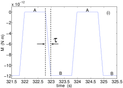
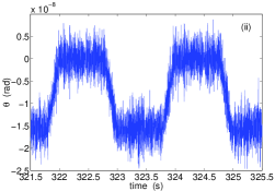
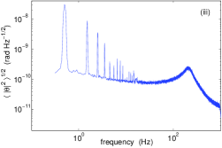
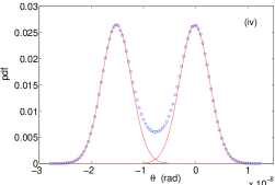
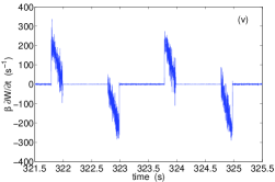
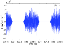
Figure 3: Oscillator immersed in oil [case (a)]: (i) Applied external torque, (ii) Induced angular displacement, (iii) its psd, (iv) its pdf, (v) Injected power computed from the Jarzynski definition $\dot{W}=-\dot{M}\theta$, (vi) Injected power computed from the standard definition $\dot{W}^{\mathrm{cl}}=-M\dot{\theta}$

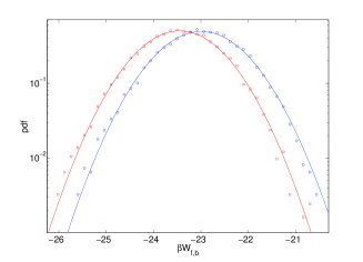
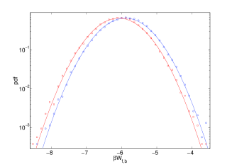
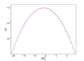
Figure 4: Case a): (i) $\mathrm{P}_{\mathrm{f}}(W)$ and $\mathrm{P}_{\mathrm{b}}(-W)$, (ii) $\mathrm{P}_{\mathrm{f}}(W^{\mathrm{cl}})$ and $\mathrm{P}_{\mathrm{b}}(-W^{\mathrm{cl}})$; Case c): (iii) $\mathrm{P}_{\mathrm{f}}(W)$ and $\mathrm{P}_{\mathrm{b}}(-W)$, (iv) $\mathrm{P}_{\mathrm{f}}(W^{\mathrm{cl}})$ and $\mathrm{P}_{\mathrm{b}}(-W^{\mathrm{cl}})$ (experimental forward and backward pdfs are represented by $\circ$ and $\Box$ respectively, whereas the continuous lines are Gaussian fits)

4 Experimental results

Now we drive the oscillator out of equilibrium between two states $A$ (where $M=0$) and $B$ (where $M=M_{m}=\mathrm{const}\neq 0$). The path $\gamma$ may be changed by modifying the time evolution of $M$ between $A$ and $B$. We have chosen either linear ramps with different rising times $\tau$, see Fig. 3(i), or half-sinusoids with half-period $\tau$. In the specific case of our harmonic oscillator, as the temperature is the same in states $A$ and $B$, the free energy difference of the oscillator alone is $\Delta F_{0}=\Delta U=\Big{[}\frac{1}{2}C\theta^{2}\Big{]}_{A}^{B}=\Big{[}\frac{M^{2}}{2C}\Big{]}_{A}^{B}$, whereas $\Delta F=\Delta F_{0}-\Big{[}\frac{M^{2}}{C}\Big{]}_{A}^{B}$, i.e. for an harmonic potential $\Delta F=-\Delta F_{0}$. Let us first consider the situation where the cell is filled with oil. The oscillator’s relaxation time is given by the inverse of the line width of the equilibrium fluctuation spectrum, see Fig. 1(ii), that is $\tau_{\mathrm{relax}}=23.5\textrm{ ms}$. We apply a torque which is a sequence of linear increasing /decreasing ramps and plateaux, as represented in Fig. 3(i). We chose different values of the amplitude of the torque $M$ [$22.1$ $11.9$, $6.1$, $4.2$ and $1.2$ pN m] and of the rising time $\tau$ [$199.5$, $20.2$, $65.6$, $99.6$, $2.5$ ms], as indicated in Table 1 [cases a)…g)] (for the case f) and g) also $C$ has been changed). Thus we can probe either the reversible (or quasi-static) paths ($\tau\gg\tau_{\mathrm{relax}}$) or the irreversible ones ($\tau\ll\tau_{\mathrm{relax}}$). We tune the duration of the plateaux (which is at least $4\,\tau_{\mathrm{relax}}$) so that the system always reaches equilibrium in the middle of each of them, which defines the equilibrium states $A$ and $B$. We see in Fig. 3(ii), where the angular displacement $\theta$ is plotted as a function of time [case a)], that the response of the oscillator to the applied torque is comparable to the thermal noise spectrum. The psd of $\theta$ is shown in Fig. 3(iii). Comparing this measure with the FDT prediction obtained in Fig. 1(ii), one observes that the driver does not affect the thermal noise spectrum which remains equal to the equilibrium one. Moreover we plot in Fig. 3(iv) the pdf of the driven displacement $\theta$ shown on Fig. 3(ii), which is, roughly speaking, the superposition of two Gaussian pdfs. From the measure of $M$ and $\theta$, the power injected into the system $\dot{W}$ can be computed from the definition given in Eq. (1), that in this case is $\dot{W}=-\dot{M}\theta$. Its time evolution, shown in Fig. 3(v), is quite different from that of the classical power $\dot{W}^{\mathrm{cl}}=-M\dot{\theta}$, whose time evolution is plotted in Fig. 3(vi): $\dot{W}$ is non-zero only for $\dot{M}\neq 0$ and vice-versa $\dot{W}^{\mathrm{cl}}\neq 0$ only for $M\neq 0$. From the time series of $\dot{W}$ we can compute from Eq. (1) the forward and the backward works, $W_{\mathrm{f}}$ and $W_{\mathrm{b}}$, corresponding to the paths $A\to B$ and $B\to A$, respectively. We also do the same for the classical work. We then compute their respective pdfs $\mathrm{P}_{\mathrm{f}}(W)$ and $\mathrm{P}_{\mathrm{b}}(-W)$. These are plotted on Figs. 4(i,iv) where the bullets are the experimental data and the continuous lines their fitted Gaussian pdfs. In Fig. 4, the pdfs of $W$ and $W^{\mathrm{cl}}$ cross in the case a) at $\beta W\simeq-23.5$, and in the case c) $\beta W\simeq-6.1$. These values correspond to $\Delta F=-\frac{M_{m}^{2}}{2C}=-\Delta F_{0}$. We find that this result is true independently of the ratio $\tau/\tau_{\mathrm{relax}}$ and of the maximum amplitude of $|M|$, $M_{m}$. This has been checked at the largest $M_{m}$ and the shortest rising time $\tau$ allowed by our apparatus. Indeed torques with amplitudes larger than $25\textrm{ pN\,m}$ and rising time shorter than $2\textrm{ ms}$ introduce mechanical noises which can be higher than thermal fluctuations and the check of the JE becomes impossible (see discussion in the next section). The measurement at very large $M_{m}$ and very short $\tau$ is shown in Fig. 5. Also in this case we see that the shape of the thermal noise spectrum is not perturbed by the driving. The pdfs remain Gaussian but the distance between ${\langle W\rangle}_{\mathrm{f}}$ and ${\langle W\rangle}_{\mathrm{b}}$ is larger and the relative variance much smaller than at low amplitude. The crossing point of the pdfs of $W$ occurs at a value where the statistics is very poor. However the two Gaussian fits crosses at $\Delta F$. The pdfs of $W^{\mathrm{cl}}$ also crosses at the right values.

(i)                                                              (ii)

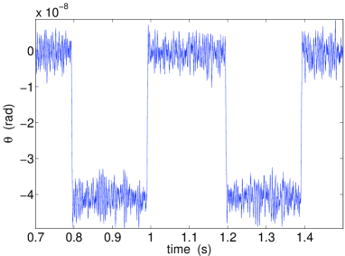
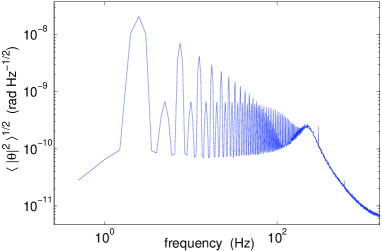
(iii)                                                              (iv)

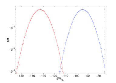
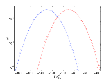
Figure 5: (i) Time evolution of $\theta$ for the case g) in Table 1, (ii) Its psd $\sqrt{\langle{|\hat{\theta}|}^{2}\rangle}$, (iii) $\mathrm{P}_{\mathrm{f}}(W)$ and $\mathrm{P}_{\mathrm{b}}(-W)$, (iv) $\mathrm{P}_{\mathrm{f}}(W^{\mathrm{cl}})$ and $\mathrm{P}_{\mathrm{b}}(-W^{\mathrm{cl}})$ (experimental forward and backward pdfs are represented by $\circ$ and $\Box$ respectively, whereas the continuous lines are Gaussian fits)

The experimental results are summarized in Table 1, where the computed $\Delta U={M_{m}^{2}\over 2C}$ is in good agreement with the values obtained by the crossing points of the forward and backward pdfs, that is $\Delta F_{\times}+\Phi$ for $\mathrm{P}(W)$ and $-\Delta W_{\times}^{\mathrm{cl}}$ for $\mathrm{P}(W^{\mathrm{cl}})$. Finally inserting the values of $W_{\mathrm{f}}$ and $W_{\mathrm{b}}$ in Eq. (2) we directly compute $\Delta F_{\mathrm{f}}$ and $\Delta F_{\mathrm{b}}$ from the JE. As it can be seen in Table 1, the values of $\Delta F_{0}$ obtained from the JE, that is either $-(\Delta F_{\mathrm{f}}+\Phi)$ or $-(\Delta F_{\mathrm{b}}+\Phi)$, agree (see sec.3.3) with the computed $\Delta U$ within experimental errors, that are about 5% on $\Delta U$ (see sec.3.3). The JE works well either when $\tau\gg\tau_{\mathrm{relax}}$ or in the critical case f) and g) where $\tau\ll\tau_{\mathrm{relax}}$. The other case we have studied is a very pathological one. Specifically, the oscillator is in vacuum and has a resonant frequency $f_{0}=353\textrm{ Hz}$ and a relaxation time $\tau_{\mathrm{relax}}=666.7\textrm{ ms}$. We applied a sinusoidal torque whose amplitude is either $5.9\times 10^{-12}$ or $9.4\times 10^{-12}\textrm{ N\,m [cases h) and i) in Table \ref{results}, respectively]}$. Half a period of the sinusoid is $\tau=49.5\textrm{ ms}$, much smaller than the relaxation time, so that we never let the system equilibrate. However, we define the states $A$ and $B$ as the maxima and minima of the driver. Surprisingly, despite of the pathological definition of the equilibrium states $A$ and $B$, the pdfs are Gaussian and the JE is satisfied as indicated in Table 1. Moreover, this happens independently of $M_{m}$ and of the critical value of the ratio $\tau/\tau_{\mathrm{relax}}\ll 1$. Finally, we indicated in Table 1 the value $\Delta F_{\circlearrowleft}$ which is the free energy computed from the JE if one considers the “loop process” from $A$ to $A$ (the same can be done from $B$ to $B$ and the results are quantitatively the same). In principle this value should be zero, but in fact it is not since we have about 3% error in the calibration of the torque $M$ and on $C$.

$\tau/\tau_{\mathrm{relax}}$	$M_{m}$	$-\beta[\Delta F_{\mathrm{f}}+\Phi]$	$\beta[\Delta F_{\mathrm{b}}+\Phi]$	$-\beta[\Delta F_{\times}+\Phi]$	$-\beta W_{\times}^{\mathrm{cl}}$	$\beta\Delta U$	$|\beta\Delta F_{\circlearrowleft}|$
$8.5^{\textrm{ a)}}$	$11.9$	$23.5$	$23.1$	$23.5$	$23.4$	$23.8$	$1.0$
$0.85^{\textrm{ b)}}$	$6.1$	$6.6$	$6.1$	$6.0$	$6.6$	$6.1$	$1.0$
$3.5^{\textrm{ c)}}$	$6.1$	$6.1$	$5.9$	$6.5$	$6.1$	$6.1$	$0.4$
$2.8^{\textrm{ d)}}$	$4.2$	$2.8$	$2.6$	$3.2$	$2.9$	$2.7$	$0.3$
$4.2^{\textrm{ e)}}$	$1.2$	$0.21$	$0.20$	$0.22$	$0.21$	$0.22$	$0.04$
$0.11^{\textrm{ f)}}$	$11.8$	$33$	$30.8$	$32.54$	$31.15$	$31.4$	$3.6$
$0.11^{\textrm{ g)}}$	$22.1$	$117.6$	$110.5$	$114$	$110.1$	$111$	$15.1$
$0.07^{\textrm{ h)}}$	$5.9$	$10.3$	$10.0$	$10.1$	$10.1$	$10.3$	$0.4$
$0.07^{\textrm{ i)}}$	$9.4$	$67.4$	$65.5$	$66.8$	$66.4$	$67.5$	$2.4$

Table 1: Free energies of cases a)…g) defined in the text (the values of $M_{m}$ are in pN m). $\Delta U={M_{m}^{2}\over 2C}$ is the computed expected value. Notice that $C=7.5\times 10^{-4}\mathrm{\ N\,m\,rad^{-1}}$ for cases a)-e), $C=5.5\times 10^{-4}\mathrm{\ N\,m\,rad^{-1}}$ for cases f)-g) and $C=1.6\times 10^{-4}\mathrm{\ N\,m\,rad^{-1}}$ for cases h)-i)

5 Jarzynski equality and the Langevin equation

In the previous section we have seen that even at very large driving torque, two properties of the systems remain unchanged, specifically: the thermal noise amplitude and statistics are not modified by the presence of the large forcing, that is FDT is still valid and the fluctuation pdf remains Gaussian. As we have already discussed, the fact that FDT is still valid is easily understood by comparing the noise spectrum of fig.1-ii) without driving with those with driving in fig.3-ii) and fig.5ii). We clearly see that the driving does not change the shape of the noise spectrum, once the pics corresponding to the driving have been subtracted. It is also easy to show that the pdf $P_{d}(\theta)$ of $\theta$, with the driving, is the convolution product of the pdf $P(\theta)$, without driving, times $P(\overline{\theta})$ which is the mean response of $\theta$ to the driving torque. As an example we show in fig.6a) $P(\theta)$ without driving. The PDF $P(\overline{\theta})$ of the mean response of $\theta$, measured for the case g) of Table 1, is plotted in fig.6b). This PDF is close to the sum of two delta functions. In fig.6c) we show, for the case g) of Table 1, the directly measured $P_{d}(\theta)$ (circles) and that computed by the convolution of $P(\overline{\theta}))$ with $P(\theta)$. The agreement is excellent. This result shows that the statistical properties of the thermal noise are those of equilibrium even when the system is driven very fast.

(i)                                     (ii)                                (iii)

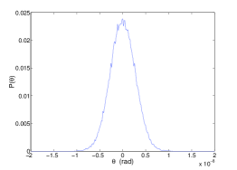
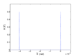
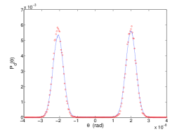
Figure 6: (i) PDF of $\theta$ when the driving is off. (ii) PDF $P(\overline{\theta})$ of the mean response of $\theta$ to the torque, measured for the case g) of Table 1. (iii) PDF $P_{d}(\theta)$ of $\theta$ measured for the case g) of Table 1 ($\circ$) and computed by the convolutions of the PDF plotted in (i) and (ii) (continuous line).

Starting from these experimental evidences, we can show that for the Langevin equation the JE is always satisfied independently of $M_{m}$ and $\tau$. Let us consider the equation for the harmonic oscillator, Eq. (16), which well describes our experimental system. In the case of a viscous damping we rewrite Eq. (16) as

$$I_{\mathrm{eff}}\,\ddot{\theta}+\nu\,\dot{\theta}+C\,\theta=M+\eta,$$ (19)

where $\eta$ is the thermal noise amplitude. For $M(t)$ we consider the kind of waveform used in the experiments:

$$M(t) = {M_{m}\,t\over\tau}\qquad\mathrm{for}\qquad 0<t<\tau,$$ (20)

$$= M_{m}\qquad\mathrm{for}\qquad t>\tau.$$ (21)

5.1 The overdamped case

In order to compute $\Delta F$ using the JE when the system is driven from $A$ ($M=0$) to $B$ ($M=M_{m}\neq 0$), we first consider the overdamped case when the inertial term is negligible, that is $I_{\mathrm{eff}}\simeq 0$:

$$\dot{\theta}+\tau_{0}^{-1}\,\theta=(C\,\tau_{0})^{-1}(M+\eta),$$ (22)

where $\tau_{0}=\nu/C$. If $\eta$ is a thermal noise, then when $M=0$ the spectrum of the thermal fluctuations $\delta\theta$ of $\theta$ can be computed from FDT:

$$\langle{|\hat{\theta}|}^{2}\rangle=\frac{4k_{B}T\,\tau_{0}}{C(1+\tau_{0}^{2}\,\omega^{2})}$$ (23)

As a consequence the autocorrelation function of $\theta$ on a time interval $\delta\tau$ is

$$R_{\theta}(\delta\tau)=\frac{k_{B}T}{C}\,\exp{\Bigl{(}-{|\delta\tau|\over\tau_{0}}\Bigr{)}}.$$ (24)

The pdf of $\theta$ is Gaussian. The work to drive the system from $A$ to $B$ computed using Eq. (1) becomes in this case

$$W=-{M_{m}\over\tau}\int_{0}^{\tau}\theta\,\mathrm{d}t$$ (25)

Thus to compute $W$ we need only the solution of Eq. (22) for $0<t<\tau$. If we neglect the noise, then the mean solution is

$$\overline{\theta}={M_{m}\over\tau\,C}\Bigl{[}t+\tau_{0}\,\exp{\Bigl{(}-{t\over\tau_{0}}\Bigr{)}}-\tau_{0}\Bigr{]}\qquad\mathrm{for}\qquad 0<t<\tau.$$ (26)

We now consider that in the experiment the statistical properties of the thermal fluctuations $\delta\theta$ are not modified by the driving. Therefore $\theta$ can be decomposed in the sum of an average part $\overline{\theta}$ given by Eq. (26) plus the fluctuating part $\delta\theta$, that is

$$\theta=\overline{\theta}+\delta\theta.$$ (27)

As a consequence the work can also be decomposed in a similar manner

$$W=\overline{W}+\delta W=-{M_{m}\over\tau}\Biggl{[}\int_{0}^{\tau}\overline{\theta}\,\mathrm{d}t+\int_{0}^{\tau}\delta\theta\,\mathrm{d}t\Biggr{]}.$$ (28)

As the integral of a Gaussian variable is still Gaussian then the fluctuations of $W$ remain Gaussian too. As a consequence, to compute $\Delta F$ we can use Eq. (8), where $\langle W\rangle$ is straightforward computed using Eqs. (26) and (28)

$$\langle W\rangle=\overline{W}=-{M_{m}\over\tau}\,\int_{0}^{\tau}\overline{\theta}\,\mathrm{d}t=-{1\over C}{\left({M_{m}\over\tau}\right)}^{2}\Bigl{[}{(\tau-\tau_{0})^{2}\over 2}-\tau_{0}^{2}\exp{\Bigl{(}-{\tau\over\tau_{0}}\Bigr{)}}+{{\tau_{0}}^{2}\over 2}\Bigr{]}.$$ (29)

We now have to compute $\sigma_{W}^{2}=\langle{(\delta W})^{2}\rangle=({M_{m}/\tau})^{2}\,\langle y^{2}(\tau)\rangle$ where

$$y(\tau)=\int_{0}^{\tau}\delta\theta\,\mathrm{d}t.$$ (30)

The variance of $y$ can be computed [24] taking into account that

$$\langle y^{2}(\tau)\rangle=\int_{0}^{\tau}\int_{0}^{\tau}R_{\theta}(t_{1}-t_{2})\,\mathrm{d}t_{1}\,\mathrm{d}t_{2}.$$ (31)

Using this equation and Eq. (24) we get

$$\sigma_{W}^{2}=\left({M_{m}\over\tau}\right)^{2}\langle y^{2}(\tau)\rangle={2k_{B}T\tau_{0}\over C}\left({M_{m}\over\tau}\right)^{2}\Bigl{[}\tau-\tau_{0}+\tau_{0}\exp{\Bigl{(}-{\tau\over\tau_{0}}\Bigr{)}}\Bigr{]}.$$ (32)

Taking into account that fluctuations of $W$ are Gaussian, we replace the results of Eqs. (29) and (32) in Eq. (8), and finally we get

$$\Delta F=\langle W\rangle-{\sigma_{W}^{2}\over 2k_{B}T}=-{M_{m}^{2}\over 2C},$$ (33)

that is the expected value. It is important to notice that this equation gives the exact result independently of the rising time of the external applied torque. This is important because it shows that the in cases where the conditions a) and b) are verified, the JE gives the right result independently of the path to go from $A$ to $B$, which can be a very irreversible one.

5.2 The harmonic oscillator

We may now repeat the calculation for the harmonic oscillator of Eq. (19). In such a case let us introduce the following notations

$$\alpha={\nu\over 2I_{\mathrm{eff}}},\qquad\alpha^{2}+\psi^{2}={C\over I_{\mathrm{eff}}},$$ (34)

and

$$\cos{\varphi}={\alpha\over\sqrt{\alpha^{2}+\psi^{2}}},\qquad\sin{\varphi}={\psi\over\sqrt{\alpha^{2}+\psi^{2}}}.$$ (35)

With this notation the mean solution of Eq. (19) in absence of noise, with initial conditions $\theta(0)=\dot{\theta}(0)=0$, is

$$\bar{\theta}={M_{m}\over\tau\psi}\Bigl{[}\exp{(-\alpha t)}\,\sin{(\psi t+2\varphi)}+\psi\,t-\sin{2\varphi}\Bigr{]}\qquad\mathrm{for}\qquad 0<t<\tau.$$ (36)

The correlation function of the thermal fluctuations $\delta\theta$ become in this case

$$R_{\theta}(\delta\tau)={k_{B}T\over C\sin{\varphi}}\,\exp{(-\alpha|\delta\tau|)}\,\sin{(\psi|\delta\tau|+\varphi)}.$$ (37)

We now proceed as in the overdamped case and we compute $\langle W\rangle$ and $\sigma_{W}^{2}$. Using Eq. (36) and Eq. (28) we get

$$\langle W\rangle=\left({M_{m}\over\tau\psi}\right)^{2}{\sin{\varphi}\over C}\left[\exp{(-\alpha\tau)}\,\sin{(\psi\tau+3\varphi)}-\sin{3\varphi}-{(\psi\tau)^{2}\over 2\sin{\varphi}}+2\psi\tau\cos{\varphi}\right]$$ (38)

To compute the variance of $W$, we insert Eq. (37) in Eq. (31) and we obtain

$$\sigma_{W}^{2} = \left({M_{m}\over\tau}\right)^{2}\langle y^{2}(\tau)\rangle$$ (39)

$$= \left({M_{m}\over\tau}\right)^{2}{2k_{B}T\sin{\varphi}\over C\psi^{2}}\left[\exp{(-\alpha\tau)}\,\sin{(\psi\tau+3\varphi)}-\sin{3\varphi}+2\psi\tau\cos{\varphi}\right].$$

As the fluctuations of $W$ are Gaussian, we insert Eqs. (38) and (39) in Eq. (8), and we obtain

$$\Delta F=\langle W\rangle-{\sigma_{W}^{2}\over 2k_{B}T}=-{M_{m}^{2}\over 2C},$$ (40)

which is the expected results. Notice that in this case too the result is independent on the path. Thus the JE gives the right result of $\Delta F$ for the Langevin equation with an harmonic potential.

6 Discussion and Conclusions

6.1 Experimental limits of JE and CR

Before concluding we want to discuss the limits on the use of JE and CR in an experiment where the dynamics can be either exactly described or well approximated by a Langevin equation. From the values of $\langle W\rangle$ and of $\sigma_{W}$, computed in sect. 4 for the overdamped case and for the harmonic oscillator case, we see that if $\tau$ is kept constant then $\langle W\rangle\propto M_{m}^{2}$ whereas $\sigma_{W}\propto M_{m}$. Furthermore as $2\,\Delta F={\langle W\rangle}_{\mathrm{f}}-{\langle W\rangle}_{\mathrm{b}}$ is proportional to $M_{m}^{2}$, this means that the distance between the maxima of $\mathrm{P}_{\mathrm{f}}(W)$ and $\mathrm{P}_{\mathrm{b}}(-W)$ increases with $M_{m}^{2}$ and the relative width $|\sigma_{W}/\langle W\rangle|$ of $\mathrm{P}(W)$ decreases as $1/M_{m}$. As a consequence, the probability of finding experimental values of $W$ close to the crossing points also decreases as $1/M_{m}$. This effect has been seen on the experimental $\mathrm{P}(W)$ plotted in Fig. 5. From a practical point of view, this means that when $\Delta F\gg k_{B}T$ the pdfs will never cross, for reasonable values of the work pdf. As a consequence the experimental test of JE and CR in systems with a strongly irreversible driving force, as proposed in ref.[11], will be very difficult to test. Indeed at such a large and fast driving, the JE and CR may fail, either for deep theoretical reasons or simply because the statistics is too poor. At the moment we are not able to answer to this question. Furthermore, for real (macroscopic) systems it is reasonable to think that when the external noise becomes much larger than the thermal noise, the JE cannot be used. However, if the pdfs of $W^{\mathrm{cl}}$ remain Gaussian, then the crossing point $W_{\times}^{\mathrm{cl}}$ gives the right result.

6.2 Summary and discussion of the results

In conclusion we have used a driven torsion pendulum to test experimentally the accuracy of JE and CR. By varying the amplitude and the rising time of the driving torque of about one order of magnitude, we clearly demonstrate the validity and the robustness of the JE and CR in an isothermal process, at least when the work fluctuations are Gaussian and when the harmonic approximation is relevant for the system. We have checked the generality of the results on a driven Langevin equation which well describes the dynamics of the oscillator. Using the experimental observations that the equilibrium properties of the thermal noise are not modified by the driving force and that the force fluctuations are Gaussian, we have shown that the JE gives the right result independently of $M_{m}$ and $\tau$. Unfortunately these results do not fully alight the theoretical debate, because our conditions are close to those pointed out in Ref. [11] for the validity of the JE. Recently, Ritort and coworkers have used the JE and CR to estimate $\Delta F$ in an experiment of RNA stretching where the oscillator’s coupling is non-linear and the work fluctuations are non-Gaussian [25]. It would be interesting to check these results on a more simple and controlled system. We are currently working on the experimental realization of such a non-linear coupling, for which $\Delta F\neq-\Delta F_{0}$.

We have also shown both analytically and experimentally that $|\sigma_{W}/\langle W\rangle|$ decreases as $1/M_{m}$. This observation makes the practical use of the JE and CR rather unrealistic for very large $M_{m}$ as the statistics needed to get a reliable result will be very large. This means, as we have already discussed at the end of the previous section, that the JE cannot be applied for macroscopic systems when the external noise becomes much larger than the thermal noise.

Going back to the estimate of $\Delta F$ we have seen that the more accurate and reliable $\Delta F$ estimator is given by the crossing points $\Delta F_{\times}$ and $W_{\times}^{\mathrm{cl}}$, because they are less sensitive to the extreme fluctuations which may perturb the convergence of the JE. Starting from this observation, we propose a new method to compute $\Delta F$ in the case of Gaussian fluctuations of $W^{\mathrm{cl}}$. Indeed, for Gaussian pdfs $W_{\times}^{\mathrm{cl}}$ remains an excellent estimator even in cases where the JE and the CR could not hold, for example when the environmental noise cannot be neglected.

Finally we want to stress that our results, although limited to the Gaussian case, show that it is possible to measure tiny work fluctuations in a macroscopic system. As a consequence it opens a lot of perspective to use the JE, the CR and the recent theorems on dissipated work (see for example [26]) to characterize the slow relaxation towards equilibrium in more complex systems, for example aging materials such as glasses or gels [27].

The authors thank L. Bellon, E.G.D. Cohen, N. Garnier, C. Jarzynski, F. Ritort and L. Rondoni for useful discussions, and acknowledge P. Metz, M. Moulin, F. Vittoz, C. Lemonias and P.-E. Roche for technical support. This work has been partially supported by the Dyglagemem contract of EEC.

References

- [1] C. Jarzynski, Phys. Rev. Lett. 78 (14), 2690 (1997)
- [2] G.E. Crooks, Phys. Rev. E 60 (3), 2721 (1999)
- [3] C. Jarzynski, J. Stat. Phys. 98 (1/2), 77 (2000)
- [4] F. Ritort, Séminaire Poincaré 2, 63 (2003)
- [5] J. Liphardt, S. Dumont, S.B. Smith, I. Ticono Jr., C. Bustamante, Science 296, 1832 (2002)
- [6] G.E. Crooks, J. Stat. Phys. 90 (5/6), 1481 (1997)
- [7] C. Jarzynski, Phys. Rev. E 56 (5), 5018 (1997)
- [8] O. Mazonka, C. Jarzynski, cond-mat/9912121 (1999)
- [9] G.E. Crooks, Phys. Rev. E 61 (3), 2361 (2000)
- [10] C. Jarzynski, D.K. Wójcik, Phys. Rev. Lett. 92 (23), 230602-1 (2004)
- [11] E.G.D. Cohen, D. Mauzerall, J. Stat. Mech.: Theor. Exp. P07006 ( 2004)
- [12] F. Douarche, S. Ciliberto, A. Petrosyan, I. Rabbiosi, An experimental test of the Jarzynski equality in a mechanical experiment, Europhys. Lett. 70, 5, 593 (2005). cond-mat/0502395
- [13] L.D. Landau, E.M. Lifshitz, Statistical Physics (Pergamon Press, 1970)
- [14] R. Peierls, Phys. Rev.54, 918 (1938)
- [15] H. Goldstein, Classical mechanics 2nd ed. (Addison Wesley, 1980)
- [16] J. Hermans, J. Phys. Chem. 95, 9029 (1991).
- [17] G. Hummer, A. Szabo, PNAS 98, 3658 (2001).
- [18] H. Lamb, Hydrodynamics (Dover, 1993)
- [19] G. Nomarski, J. Phys. Radium 16, 9S (1954)
- [20] L. Bellon, S. Ciliberto, H. Boubaker, L. Guyon, Opt. Commun. 207, 49 (2002)
- [21] L. Bellon, L. Buisson, S. Ciliberto, and F. Vittoz, Rev. Sci. Instr.,(73), 9, 3286 (2004)
- [22] F. Douarche, L. Buisson, S. Ciliberto, A. Petrosyan, Rev. Sci. Instr. 75 (12), 5084 (2004)
- [23] C. Jarzynski, J. Stat. Mech.: Theor. Exp. P09005 (2004)
- [24] A. Papoulis, Probability, Random Variables and Stochastic Processes, 3rd ed. (McGraw-Hill, New York, 1991).
- [25] F. Ritort (private communication)
- [26] R. van Zon, E.G.D. Cohen, Phys. Rev. Lett. 91 (11), 110601-1 (2003)
- [27] A. Crisanti, F. Ritort, Europhys. Lett. 66 (2), 253 (2004)