Scaling of Entanglement Entropy in the Random Singlet Phase

Abstract

We present numerical evidences for the logarithmic scaling of the entanglement entropy in critical random spin chains. Very large scale exact diagonalizations performed at the critical XX point up to $L=2000$ spins $\frac{1}{2}$ lead to a perfect agreement with recent real-space renormalization-group predictions of Refael and Moore [Phys. Rev. Lett. 93, 260602 (2004)] for the logarithmic scaling of the entanglement entropy in the Random Singlet Phase with an effective central charge ${\tilde{c}}=c\times\ln 2$. Moreover we provide the first visual proof of the existence the Random Singlet Phase with the help of quantum entanglement concept.

The study of quantum phase transitions through quantum entanglement concepts provides a new way to understand strongly correlated systems near criticality. In one dimensional systems, such as quantum spin chains, entanglement estimators exhibit universal features close to a critical point Nature ; Vidal03 . One of this estimator is the entanglement entropy of a subsystem A with respect to a subsystem B. Defined as the Von Neumann entropy of the reduced density matrix for either subsystem

$${\mathcal{S}}=-Tr{\hat{\rho}}_{A}\ln{\hat{\rho}}_{A}=-Tr{\hat{\rho}}_{B}\ln{\hat{\rho}}_{B},$$ (1)

this quantity displays very interesting scaling behavior for conformally invariant critical theories in one dimension (1D). Indeed, as shown first by Holzey, Larsen and Wilczek HLW94 in the context of geometric entropy related to black hole physics, the entanglement entropy of a subsystem of length $x$ embedded in an infinite system is expected to scale like

$${\mathcal{S}}(x)\sim\frac{c}{3}\ln x.$$ (2)

The number $c$ is the so-called central charge which is, for instance, for the critical XXZ spin-$\frac{1}{2}$ chain $c_{\rm XXZ}=1$ or for the spin-$\frac{1}{2}$ Ising chain in transverse field at criticality $c_{\rm Ising}=1/2$. This result [Eq. (2)] has been verified numerically Vidal03 ; Vidal04 as well as analytically in Ref. Korepin04 where some simple connections have been established between thermodynamic entropy and entanglement entropy. An important extension to critical and non-critical systems with finite size, finite temperature and different boundary conditions has been achieved by Calabrese and Cardy Cardy04 . They showed for instance that for critical systems of finite size $L$ with periodic boundary conditions, Eq. (2) should be replaced by

$${\mathcal{S}}(L,x)=\frac{c}{3}\ln\left(\frac{L}{\pi}\sin(\frac{\pi x}{L})\right)+{\rm{s_{1}}},$$ (3)

where $s_{1}$ is a constant related to the UV cut-off.

Although such a logarithmic scaling of the entanglement entropy seems closely related to the conformal invariance of the critical system, it has been shown recently by Refael and Moore Refael04 that such a critical scaling is also expected for some random critical points. Indeed, using an analytic real-space renormalization-group (RSRG) approach, they have shown that random critical spin chains display similar features that clean ones with an effective central charge ${\tilde{c}}=c\times\ln 2$ so that

$${\mathcal{S}}(x)=\frac{{\tilde{c}}}{3}\ln x+{\rm{constant}}.$$ (4)

This surprising results can be derived using the RSRG method introduced by Ma, Dasgupta and Hu Ma several years ago to study random spin chains. As a result, any amount of randomness introduced as a perturbation in a clean XXZ critical spin-$\frac{1}{2}$ chain is relevant note1 and drives the system to the so-called Random Singlet Phase (RSP) Fisher , associated with an infinite randomness fixed point (IRFP) for the RSRG transformation Fisher . The RSP can be depicted as a collection of singlet bonds of arbitrary length (see Fig. 1).

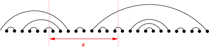
Figure 1: Schematic picture for the entanglement entropy of a subsystem of length $x$ in the random singlet phase. The entanglement is just due to the singlets connecting the subsystem with the rest of the chain. In this picture, ${\mathcal{S}}(x)=5\times\ln 2$.

Then, utilizing the very simple result that the entanglement entropy of a spin $\frac{1}{2}$ involved in a singlet with its partner is $\ln 2$, in the RSP the entanglement of a segment with the rest of the system is just given by $\ln 2$ times the number of singlets which cross the boundary of the segment, as depicted in Fig. 1. Using this fact as well as an accurate RSRG calculation, Refael and Moore have then been able to determine precisely that the number of singlets connecting a segment of size $x$ with the rest of the system is $(1/3)\ln x$, leading to the formula (4). The purpose of this communication is to investigate numerically the entanglement of the RSP and compare the RSRG prediction [Eq. (4)] with exact computations.

Exact computation of the entanglement entropy — In order to compute the entanglement entropy of a subsystem, one needs to calculate the corresponding reduced density matrix. For general XXZ spin chains governed by

$${\cal{H_{\rm{XXZ}}}}=J\sum_{j}\left[\frac{1}{2}\left(S_{j}^{+}S_{j+1}^{-}+S_{j}^{-}S_{j+1}^{+}\right)+\Delta S_{j}^{z}S_{j+1}^{z}\right],$$ (5)

the non-critical regime (achieved if $|\Delta|>1$) can be investigated using the corner transfer matrices of the corresponding two-dimensional (2D) classical problem Baxter ; Peschel1 . On the other hand, along the critical line ($-1\leq\Delta\leq 1$), an analytical computation of ${\mathcal{S}}(x)$ is more difficult and conformal field theory (CFT) tools are then required Cardy04 . Another alternative consists in performing numerical exact diagonalizations (ED) of finite lengths spin chains, but it is limited to $L_{\rm{max}}\simeq 40$ spins $\frac{1}{2}$ when $\Delta\neq 0$ Andreas . Nevertheless, the XX point $\Delta=0$ is special because the spin Hamiltonian can be rewritten using the Jordan-Wigner transformation as a free-fermions model

$${\cal{H}}_{\rm{XX}}=\frac{J}{2}\sum_{j}\left[c_{j}^{\dagger}c_{j+1}+c_{j+1}^{\dagger}c_{j}\right]$$ (6)

for which the density matrix can be expressed as the exponential of a free-fermion operator Chung01 . It turns out that the reduced density matrix is completely determined by the $x\times x$ correlation matrix ${\mathcal{C}}(x)$, defined by

$${\mathcal{C}}(x)~{}=~{}\begin{pmatrix}\langle c^{\dagger}_{1}c_{1}\rangle&\langle c^{\dagger}_{1}c_{2}\rangle&\cdots&\langle c^{\dagger}_{1}c_{x}\rangle\\ \langle c^{\dagger}_{2}c_{1}\rangle&\langle c^{\dagger}_{2}c_{2}\rangle&\ddots&\vdots\\ \vdots&&\ddots&\\ &&&\langle c^{\dagger}_{x}c_{x}\rangle\end{pmatrix}.$$ (7)

The matrix elements ${\mathcal{C}}_{ij}=\langle c^{\dagger}_{i}c_{j}\rangle$ can be calculated either numerically by diagonalizing the free-fermion Hamiltonian in momentum space or analytically in some special cases Peschel2 . The entanglement entropy of a subsystem of size $x$ embedded in a larger system is then given by

$${\mathcal{S}}(x)=-\sum_{k}\left[\lambda_{k}\ln\lambda_{k}+(1-\lambda_{k})\ln(1-\lambda_{k})\right],$$ (8)

where the $\lambda_{k}$ are the eigenvalues of ${\mathcal{C}}(x)$.

Let us now concentrate on the disordered XX spin-$\frac{1}{2}$ chain, governed by the random hopping Hamiltonian on a periodic ring of length $L$

$${\cal{H}}_{\rm{XX}}=\sum_{j=1}^{L-1}J_{j}\left[c_{j}^{\dagger}c_{j+1}+c_{j+1}^{\dagger}c_{j}\right]$$

$$+J_{L}\exp(i\pi{\cal{N}})(c_{L}^{\dagger}c_{1}+c_{1}^{\dagger}c_{L})\$$ (9)

where $J_{j}$ are positive random numbers chosen in a flat uniform distribution within the interval $[0,1]$ note2 , and the second term in the right hand side ensures that periodic boundary conditions are imposed in the spin problem. The total number of fermions is ${\cal N}=L/2$ in the ground-state (GS). The way to diagonalize ${\cal{H}}_{\rm{XX}}$ is straightforward and has already been explained by several authors LSM61 ; Henelius98 . As a check, we have first computed the entanglement entropy (8) for clean systems (i.e. $J_{i}$ is a constant) of total sizes $L=500$ and $L=2000$. Technically, this only involves computing the elements $\langle c_{i}^{\dagger}c_{j}\rangle$ by diagonalizing the free-fermions Hamiltonian (6), and then one needs to diagonalize $\cal C$ [Eq. (7)] using standard linear algebra routines LAR .

\psfrag{A}{\tiny{$0.8595+\frac{\ln 2}{3}\ln x$}}\psfrag{Y}{\tiny{$0.72602+\frac{1}{3}\ln\left(\frac{2000}{\pi}\sin(\frac{\pi x}{2000})\right)$}}\psfrag{Z}{\tiny{$0.72587+\frac{1}{3}\ln\left(\frac{500}{\pi}\sin(\frac{\pi x}{500})\right)$}}\psfrag{E}{${\mathcal{S}}(L,x)$}\psfrag{T}{$x$}\includegraphics[width=216.81pt,height=184.9429pt,clip]{W2.eps}

Figure 2: (color online) Entanglement entropy of a subsystem of size $x$ embedded in a closed ring of size $L$, shown vs $x$ in a log-linear plot. Numerical results obtained by exact diagonalizations performed at the XX point. For clean non random systems with $L=500$ and $L=2000$ (open circles), ${\mathcal{S}}(x)$ is perfectly described by Eq. (3) (red and blue curves). The data for random systems have been averaged over $10^{4}$ samples for $L=500,~{}1000,~{}2000$ and $2\times 10^{4}$ samples for $100\leq L\leq 400$. The expression $0.8595+\frac{\ln 2}{3}\ln x$ (dashed line) fits the data in the regime where finite size effects are absent.

The results are shown in Fig. 2 where we can see that ${\mathcal{S}}(L,x)$ is perfectly described by the CFT prediction Eq. (3). Note also that the constant term is found to be $s_{1}\simeq 0.726$, in excellent agreement with the recent analytical prediction of Jin and Korepin Korepin2 .

For the random case, the same technique has been used but a bigger computational effort was necessary to average over a large number of independent random samples. Practically the number of samples used was $2\times 10^{4}$ for $L=100,~{}200,~{}300,~{}400$ and $10^{4}$ for $L=500,~{}1000,~{}2000$ which required 2000 hours of CPU computational time. The results for the disorder averaged entanglement entropy are shown in Fig. 2 When the subsystem size $x$ is large enough (typically $x>20$), the expression (4) derived by Refael and Moore describes perfectly the behavior of the disorder average entanglement entropy, i.e. a logarithmic scaling with an effective central charge ${\tilde{c}}=\ln 2$. One can notice that when the subsystem size approaches $L/2$ some finite size effects are visible, as it is the case in clean systems.

Signature of the Random Singlet Phase — The very good agreement found between exact numerical diagonalizations and RSRG calculations for the entanglement properties in the RSP is a new proof in favor of the random singlet nature of the GS, also supported by recent neutron scattering experiments performed on the disordered spin chain compound BaCu₂(Si_0.5Ge_0.5)₂O₇ Masuda04 . Another way to get more insight on these long distance effective singlets in the GS consists in looking at the probability distribution of the entanglement entropy. Indeed, since each singlet is expected to contribute as a $\ln 2$ in the entanglement entropy, we can focus on the probability distribution of ${\cal{S}}/\ln 2$ for a given subsystem embedded in a larger system. In order to get a correct statistical picture for the typical behavior of this random singlets formation, one needs a huge number of disordered samples. We chose to study $10^{5}$ independent realizations. The price to pay is that not too large systems can then be diagonalized. Nevertheless, only focusing on $L=100$ spins is enough to get good insights on the RSP. Indeed, instead of increasing the system size to achieve the physics of the RSP, according to the disorder induced crossover phenomena observed for the RSRG flow comment03 one can rather keep $L$ fixed and increase the disorder strength to get closer to the IRFP and therefore deeper in the RSP. Let us thus consider strong disorder distributions for the couplings $J_{i}$, like

$${\cal{P}}(J)=\frac{1}{\delta}J^{-1+\delta^{-1}},$$ (10)

parametrized by a disorder strength $\delta\geq 1$. This distribution is quite natural to mimic strong disorder effects since at the IRFP, the fixed point distribution for the random couplings is achieved for $\delta\to\infty$.

\psfrag{A}{{(c) $\delta=5$}}\psfrag{B}{{(d) $\delta=10$}}\psfrag{C}{{(b) $\delta=2.5$}}\psfrag{D}{{(a) $\delta=1$}}\psfrag{E}{\Large{${{\mathcal{S}}}/{\ln 2}$}}\psfrag{P}{{\Large{$P^{{\rm{even}},{\rm{odd}}}$}}}\includegraphics[width=216.81pt,clip]{E-O.Stat.eps}

Figure 3: (color online) Probability distribution for the entanglement entropy in the random singlet phase for the disordered XX spin-$\frac{1}{2}$ chain obtained by exact diagonalizations on $L=100$ spin chains. Green histograms correspond to an even subsystem size with $50$ sites ($P^{\rm{even}}=P({\cal{S}}(100,50)/\ln 2)$) and red histograms correspond to an odd subsystem with $49$ sites ($P^{\rm{odd}}=P({\cal{S}}(100,49)/\ln 2)$). For each disorder strength, $\delta=1$ (a), $\delta=2.5$ (b), $\delta=5$ (c), $\delta=10$ (d), $10^{5}$ different random samples have been diagonalized. The insets show the combined distributions $P^{\rm{even}}+P^{\rm{odd}}$. Note that all the distribution functions have been normalized to unity.

I order to minimize the finite size effects, we consider half of the chain as a subsystem and compute ${\mathcal{S}}(L,L/2)$ for each sample. Nevertheless, in order to get a good understanding, it is important to notice that the parity of $L/2$ is crucial. Indeed if $L/2$ is odd only an odd number of random singlets can connect both subsystems whereas if $L/2$ is even, the number of cut singlets will be even, none singlet being also a possibility. This fact is actually clearly visible in Figs. 3 where we have plotted the probability distributions $P^{\rm{even}}=P({\mathcal{S}}(100,50)/\ln 2)$ (green histogram) as well as $P^{\rm{odd}}=P({\mathcal{S}}(100,49)/\ln 2)$ (red histogram), for $\delta=1,~{}2.5,~{}5,~{}10$. Whereas for $\delta=1$ (Fig. 3(a)) $P^{{\rm{even}}}$ ($P^{{\rm{odd}}}$) displays an integer-peaks structure, signature of the RSP, only for ${\cal{S}}/\ln 2=2$ (${\cal{S}}/\ln 2=3$) and that a non-negligible statistical weight lies between for non-integer values, when the disorder strength increases, the integer-peaks structure becomes more and more pronounced as visible in Figs. 3(b-d). The combined distributions $P^{\rm{even}}+P^{\rm{odd}}$ are also plotted in the insets of Figs. 3. Thanks to the entanglement entropy, we provide a clear visual proof for the RSP.

Discussion and conclusion — Non disordered critical spin chains can be described by a conformally invariant field theory from which an universal number $c$, the central charge, emerges. This central charge, also called conformal anomaly number, appears in the leading finite size (or finite temperature) correction to the free energy Ian86 as well as in the entanglement entropy (3). The power-law behavior for the spin-spin correlations functions is also universal with well defined critical exponents LutherPeschel as well as exact amplitudes Amplitude .

In the case of random critical chains, while the RSRG framework provides universal critical exponents, the amplitudes of correlations functions are non-universal numbers Fisher-Young . On the other hand, the RSRG treatment for the entanglement entropy provides the exact prefactor equal to $\frac{\ln 2}{3}$. This prediction has been checked numerically using exact numerical diagonalizations on large scale random critical spin chains. The perfect agreement between exact simulations and the perturbative RSRG provides, to the best of our knowledge, the first example of an exact critical amplitude computed within this technique. It is also interesting to notice that this finding of ${\tilde{c}}=\ln 2<1$ would be consistent with a generalized ${\tilde{c}}-$theorem built on entanglement concepts for non conformal random critical points Refael04 . Nevertheless, the identificaton of other physical quantities besides entanglement that are controlled by this number ${\tilde{c}}$ turns out to be very challenging and more subtle than using a simple analogy with the clean case. Indeed, since in conformally invariant clean systems a non universal velocity factor appears tied to $c$ in the usual thermodynamic quantities like the specific heat Ian86 or the aforementioned correction to the free energy, the analogy here breaks down because the velocity of excitations is not defined anymore in the RSP.

To conclude, we believe that the results presented in this communication provide a new insight on the random singlet phase as well as a first visual proof of the large scale effective singlets formation. The fact that even at the infinite randomness fixed point the entanglement entropy still scales logarithmically with the subsystem size provides a non trivial extension of the quantum entanglement concepts to random quantum critical points.

I would like to thank Ian Affleck, Ming-Shyang Chang, Joel Moore, and Gil Refael for stimulating and interesting discussions, as well as Ingo Peschel and Vladimir Korepin for correspondence. I also thank NSERC of Canada for financial support and WestGrid for access to computational facilities.

References

- (1) A. Osterloh, L. Amico, G. Falci, and R. Fazio, Nature (London) 4126, 608 (2002).
- (2) G. Vidal, J. I. Latorre, E. Rico, and A. Kitaev, Phys. Rev. Lett. 90, 227902 (2003).
- (3) C. Holzhey, F. Larsen, and F. Wilczek, Nucl. Phys. B 424 44 (1994).
- (4) J. I. Latorre, E. Ricco, and G. Vidal, Quant. Inf. and Comp. 4, 048 (2004).
- (5) V. E. Korepin, Phys. Rev. Lett. 92, 096402 (2004).
- (6) P. Calabrese and J. Cardy, J. Stat. Mech. 06 (2004) 002.
- (7) G. Refael and J. E. Moore, Phys. Rev. Let. 93, 260602 (2004).
- (8) S.-k. Ma, C. Dasgupta, and C.-k. Hu, Phys. Rev. Lett. 43, 1434 (1979); C. Dasgupta and S.-k. Ma, Phys. Rev. B 22, 1305 (1980).
- (9) D. S. Fisher, Phys. Rev. B 50, 3799 (1994); D. S. Fisher, Phys. Rev. Lett. 69, 534 (1992); D. S. Fisher, Phys. Rev. B 51, 6411 (1995).
- (10) To be more precise, this is only true when the anisotropy ; see C. A. Doty and D. S. Fisher, Phys. Rev. B 45, 2167 (1992).
- (11) I.Peschel, M.Kaulke and O.Legeza, Ann. Physik (Leipzig) 8, 153 (1999).
- (12) R. J. Baxter, Exactly Solved Models in Statistical Mechanics, Academic Press, London (1982).
- (13) A. M. Laüchli: “Quantum magnetism and strongly correlated electrons in low dimension”, PhD Thesis, Swiss Federal Institute of Technology, Zürich (2002).
- (14) M.-C. Chung and I. Peschel, Phys. Rev. B 64, 064412 (2001; I. Peschel, J. Phys. A 36, L205 (2003); I. Peschel, J. of Statistical Mechanics P06004 (2004).
- (15) I. Peschel, J. Phys. A: Math. Gen. 38, 4327 (2005).
- (16) Note that we have also simulated less disordered systems with narrower distributions but the conclusions do not change, except for some finite size crossover phenomena already discussed in Ref. comment03 for the correlation functions.
- (17) N. Laflorencie and H. Rieger, Phys. Rev. Lett 91, 229701 (2003); N. Laflorencie, H. Rieger, A. W. Sandvik, and P. Henelius, Phys. Rev. B 70, 054430 (2004).
- (18) E. Lieb, T. Schulz, and D. Mattis, Ann. Phys. (NY) 16, 407 (1961).
- (19) P. Henelius and S. M. Girvin, Phys. Rev. B 57, 11457 (1998).
- (20) The linear algebra package LAPACK has been used here.
- (21) B.-Q. Jin and V. E. Korepin, J. Stat. Phys. 116, 79 (2004).
- (22) T. Masuda, A. Zheludev, K. Uchinokura, J.-H. Chung, and S. Park Phys. Rev. Lett. 93, 077206 (2004).
- (23) H. W. J. Blöte, J. L. Cardy, and M. P. Nightingale, Phys. Rev. Lett. 56, 742 (1986); I. Affleck, Phys. Rev. Lett. 56, 746 (1986).
- (24) A. Luther and I. Peschel, Phys. Rev. B 12, 3908 (1975).
- (25) I. Affleck, J. Phys. A 31, 4573 (1998); S. Lukyanov, Phys. Rev. B 59, 11163 (1999).
- (26) D. S. Fisher and A. P. Young, Phys. Rev. B 58, 9131 (1998).