Determination of the magnetic domain size in the ferromagnetic superconductor UGe₂ by three dimensional neutron depolarization

Abstract

Three dimensional neutron depolarization measurements have been carried out on single-crystalline UGe₂ between 4 K and 80 K in order to determine the average ferromagnetic domain size $d$. It is found that below $T_{C}=52$ K uniaxial ferromagnetic domains are formed with an estimated magnetic domain size of $d\approx 4-5~{}\mu$m.

I Introduction

Recently, the compound UGe₂ has attracted much attention because superconductivity was found to coexist with ferromagnetism. Saxena et al. (2000); Aoki et al. (2001) Until this discovery, only superconducting compounds exhibiting antiferromagnetic order had been known like DyMo₆S₈, GdMo₆S₈, and TbMo₆S₈. Moncton et al. (1978); Majkrzak et al. (1979); Thomlinson et al. (1981) Coexistence of antiferromagnetism and superconductivity was also found in the heavy fermion compounds like CeIn₃, CePd₂Si₂, and UPd₂Al₃. Walker et al. (1997); Grosche et al. (1997); Sato et al. (2001) In these cases superconductivity and antiferromagnetism appear simultaneously, because the Cooper pairs are insensitive to the internal fields arising from the antiferromagnetic ordering when the superconducting coherence length $\xi$ is much larger than the periodicity of the static antiferromagnetic ordered structure. However, in a ferromagnetic structure we expect that the internal fields do not cancel out on the length scale of $\xi$ and therefore have their influence on the Cooper pairs. That ferromagnetic order excludes superconductivity, is nicely demonstrated in ErRh₄B₄ Fertig et al. (1977); Moncton et al. (1980) and HoMo₆S₈ Ishikawa and Fischer (1977), where standard BCS singlet-type superconductivity is suppressed when ferromagnetic order sets in. Otherwise, if one would consider unconventional spin-triplet superconductivity mediated by ferromagnetic spin fluctuations, the pairing is relatively insensitive to a local magnetic field and can therefore coexist with ferromagnetic order. On the other hand, when the ferromagnetic domain size $d$ is much smaller than the superconducting coherence length $\xi$, one effectively has no internal magnetic field.

The coherence length $\xi$ for UGe₂ is estimated Saxena et al. (2000); Tateiwa et al. (2001) to be 130-200 Å. Interestingly, Nishioka et al.Nishioka et al. (2002, 2003), considering jumps in the magnetization at regular intervals of magnetic field and at very low temperatures, estimated the ferromagnetic domain size $d$ to be of the order of 40 Å, by attributing the jumps to field-tuned resonant tunnelling between quantum spin states. Since $d$ would be several times smaller than $\xi$, it was proposed that the ferromagnetism can be cancelled out on the scale of the coherence length of the Cooper pairs. This would imply that the pairing mechanism for superconductivity might be of the singlet-type after all.

UGe₂ crystallizes in the orthorhombic ZrGa₂ crystal structure (space group Cmmm) Boulet et al. (1997) with unit cell dimensions $a=4.036$ Å, $b=14.928$ Å, and $c=4.116$ Å, containing 4 formula units. Ferromagnetic order sets in at $T_{C}=52$ K. The saturated magnetic moment at ambient pressure is $1.4~{}\mu_{\mathrm{B}}$/U, directed along the $\bf a$ axis. Magnetic measurements indicate a very strong magnetocrystalline anisotropy. Onuki et al. (1992) Superconductivity is found only in a limited pressure range between 10 and 16 kbar with a maximum transition temperature of $T_{c}\approx 0.7$ K. In this pressure range, the magnetic moment is still $1~{}\mu_{\mathrm{B}}$/U. Within the ferromagnetic phase, a second transition occurs at $T_{X}\sim 25$ K at ambient pressure, below which the magnetic moment is enhanced. Therefore the temperature region from $T_{C}$ to $T_{X}$ was named the weakly polarized phase, while the lower temperature region $T<T_{X}$ was called the strongly polarized phase. Huxley et al. (2000)

In this paper we report on three dimensional neutron depolarization measurements performed on single-crystalline UGe₂ at ambient pressure between 4 K and 80 K. Our principal aim was to determine the ferromagnetic domain size $d$ in UGe₂ and compare the value to the size of $\sim 40$ Å estimated by Nishioka et al.Nishioka et al. (2002) on the basis of the hypothesis of field-tuned resonant tunnelling between spin quantum states. Since the neutron is a very sensitive probe to local magnetic fields, neutron depolarization is an excellent technique to measure the average domain size and the domain wall width.

II Experiment

II.1 Experimental

The measurements were performed on the Poly Axis Neutron Depolarization Analyzer (PANDA) at the Interfaculty Reactor Institute (IRI) of the Delft University of Technology. The used neutron wave length was 2.03 Å which corresponds to a velocity of 1949 m/s.

The neutron depolarization measurements on UGe₂ were performed on a single-crystalline sample with dimensions $a\times b\times c=4.0\times 0.440\times 3.0$ mm³. The $\bf b$ axis was oriented along the transmitted neutron beam ($x$) with a transmission length $L$ and the easy axis for magnetization a along the vertical axis ($z$) within the plate of the sample. The crystal has been grown from a polycrystalline ingot using a Czochralski tri-arc technique. No subsequent heat treatment was given to the crystal. The illuminated area was a rectangle with dimensions $y\times z=1\times 2$ mm² centered at the middle of the sample.

The measurements in zero field were performed during a temperature sweep from 2 K up to 80 K and down to 2 K with a low sweep rate of 10 K/hr. The measurements in non-zero field (4 and 8 mT) were done during a similar temperature sweep with a sweep rate of 25 K/hr. The sample was first zero-field cooled, whereafter the field was switched on at the start of the measurements. The subsequent measurements were performed during heating and cooling in a constant field.

II.2 Neutron depolarization

The neutron depolarization (ND) technique is based on the loss of polarization of a polarized neutron beam after transmission through a (ferro)magnetic sample. Each neutron undergoes only a series of consecutive rotations on its passage through the (ferro)magnetic domains in the sample. It is important to note that the beam cross section covers a huge number of domains, which results in an averaging over the magnetic structure of the whole illuminated sample volume. This averaging causes a loss of polarization, which is determined by the mean domain size and the mean direction cosines of the domains. The rotation of the polarization during transmission probes the average magnetization.

The $3\times 3$ depolarization matrix $D$ in a ND experiment expresses the relation between the polarization vector before ($\vec{P}^{0}$) and after ($\vec{P}^{1}$) transmission through the sample ($\vec{P}^{1}=D\vec{P}^{0}$). The polarization of the neutrons is created and analyzed by magnetic multilayer polarization mirrors. In order to obtain the complete matrix $D$, one polarization rotator is placed before the sample and another one right after the sample. Each rotator provides the possibility to turn the polarization vector parallel or antiparallel to the coordinate axes $x$, $y$, and $z$. The resultant neutron intensity is finally detected by a ³He detector. The polarization rotators enable us to measure any matrix element $D_{ij}$ with the aid of the intensity of the unpolarized beam $I_{S}$:

$$I_{S}=\frac{I_{ij}+I_{-ij}}{2}.$$ (1)

where $I_{ij}$ is the intensity for $\vec{P}^{0}$ along $i$ and $\vec{P}^{1}$ along $j$. The matrix element $D_{ij}$ is then calculated according to

$$D_{ij}=\frac{1}{P_{0}}\,\frac{I_{S}-I_{ij}}{I_{S}}$$ (2)

where $P_{0}$ is the degree of polarization in the absence of a sample. In our case we have $P_{0}=0.965$.

We now introduce the correlation matrix $\alpha_{ij}$:

$$\alpha_{ij}=\Big{<}\int_{0}^{L}\!\!\!\!dx^{\prime}\Delta B_{i}(x,y,z)\Delta B_{j}(x^{\prime},y,z)\Big{>},$$ (3)

where $\Delta\vec{B}(\vec{r})=\vec{B}(\vec{r})-\langle\vec{B}\rangle$ is the variation of the magnetic induction, $\langle\ldots\rangle$ denotes the spatial average over the sample volume and where the integral is over the neutron transmission length $L$ through the sample. Assuming $\alpha_{ij}\equiv 0$ for $i\neq j$ we define the correlation function $\xi$ as

$$\xi=\sum_{i}\alpha_{ii}.$$ (4)

With these two quantities it can be shown that if there is no macroscopic magnetization ($\langle\vec{B}\rangle$ = 0) the depolarization matrix is diagonal and under the assumption of $\alpha_{ij}\equiv 0$ for $i\neq j$ given by Rekveldt (1973); Rosman and Rekveldt (1990, 1991)

$$D_{ii}=e^{-\frac{\gamma^{2}}{v^{2}}L\left\{\xi-\alpha_{ii}\right\}}\mbox{\hskip 28.45274pt}i=x,y,z.$$ (5)

where $\gamma=1.83\times 10^{8}$ s^-1T^-1 is the gyromagnetic ratio of the neutron and $v$ its velocity.

Intrinsic anisotropy is the depolarization phenomenon that for magnetically isotropic media the depolarization depends on the orientation of the polarization vector with respect to the propagation direction of the neutron beam. The origin of this intrinsic anisotropy is the demagnetization fields around magnetized volumes in the sample. In the following we will assume that the demagnetization fields are negligible for needle shaped magnetic domains.

We now discuss the case $\langle\vec{B}\rangle\neq 0$. When the sample shows a net magnetization, the polarization vector will rotate in a plane perpendicular to the magnetization direction. If the sample shape gives rise to stray fields, the rotation angle $\phi$ is related to the net magnetization $\langle M\rangle$ by

$$\phi=\eta\frac{\gamma}{v}L\mu_{0}\langle M\rangle=\eta\frac{\gamma}{v}L\mu_{0}M_{S}\langle m\rangle$$ (6)

where $\eta$ is a geometrically factor given in Eq. 27 for a rectangular shaped sample and $\langle m\rangle=M/M_{S}$ the reduced sample magnetization in terms of the saturation magnetization $M_{S}=M_{S}(T)$. If the mean magnetic induction $\langle\vec{B}\rangle$ in the sample is oriented along the $z$-axis, the depolarization matrix is, for $\phi\gg\left(\gamma/v\right)^{2}\left|\alpha_{xx}-\alpha_{yy}\right|L/2$ (the weak damping limit), given by Rekveldt (1973); Rosman and Rekveldt (1990, 1991)

$$D_{xx}=D_{yy} = e^{-\frac{\gamma^{2}}{v^{2}}L\left\{\xi-\frac{\alpha_{xx}+\alpha_{yy}}{2}\right\}}\cos\phi,$$

$$D_{xy}=-D_{yx} = e^{-\frac{\gamma^{2}}{v^{2}}L\left\{\xi-\frac{\alpha_{xx}+\alpha_{yy}}{2}\right\}}\sin\phi,$$

$$D_{zz} = e^{-\frac{\gamma^{2}}{v^{2}}L\left\{\xi-\alpha_{zz}\right\}},$$

$$D_{xz}=D_{zx} = D_{zy}=\ D_{yz}=0.$$

With the net magnetization along the $z$-axis, the rotation angle $\phi$ of the beam polarization is obtained from the measurements by

$$\phi=\arctan\left(\frac{D_{xy}-D_{yx}}{D_{xx}+D_{yy}}\right)$$ (8)

and $\xi$ is calculated with

$$\xi=-v^{2}\ln\left\{\det D\right\}/2\gamma^{2}L.$$ (9)

As mentioned earlier, ND also provides information about the mean-square direction cosines of the magnetic induction vector in the (ferro)magnetic domains. These are directly given by the quantities $\gamma_{i}=\alpha_{ii}/\xi$, where $i=x,y,z$, and can be estimated from the measurements by

$$\gamma_{i}=1-2\ln D_{ii}/\ln\left\{\det D\right\}.$$ (10)

This equation is only valid for those directions which show no net rotation of the beam polarization.

III results

III.1 Measurements in zero field

In Fig. 1

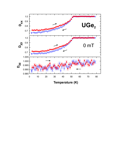
Figure 1: The diagonal elements of the measured depolarization matrix $D$ for increasing and decreasing temperature for UGe₂. All other elements of the depolarization matrix are zero within the experimental uncertainty. For $D_{xx}$ and $D_{yy}$ the experimental uncertainty is within the symbol size.

we show the diagonal elements of the depolarization matrix for UGe₂, measured in zero magnetic field. All off-diagonal elements are zero within the experimental uncertainty in the studied temperature range. The measurements for increasing temperature are qualitatively the same as those for decreasing temperature, as expected.

The Curie temperature of $T_{C}=52$ K is clearly indicated in Fig. 1 by the kink in $D_{xx}$ and $D_{yy}$. Note that $D_{xx}\equiv D_{yy}$ below $T_{C}$ indicates that there is no intrinsic anisotropy and hence that the magnetic domains produce virtually no stray fields. Furthermore, $D_{zz}\approx 1$ indicates that all moments are oriented along the $\bf a$ axis.

III.2 Measurements in small field

In Fig. 2

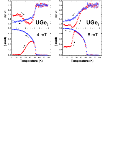
Figure 2: The determinant of the measured depolarization matrix $\det D$ and the rotation angle $\phi$ of the beam polarization after passage through the sample of UGe₂ in 4 mT and 8 mT for increasing and decreasing temperature.

we show the determinant of the depolarization matrix $\det D$ and the rotation angle $\phi$ after passage through the sample for measurements in fields of respectively 4 and 8 mT (after zero-field cooling). The data of $\phi$ have been corrected by subtracting the mean value above $T_{C}$, since this rotation is merely due to the applied field.

At low temperatures the magnetic fields (applied after zero field cooling) are too small to fully align the magnetic domains. Therefore, the measurements for increasing and decreasing temperature do not yield the same results. Whereas for increasing temperature the rotation shows an increase, for decreasing temperature the data represent a monotonous magnetization curve, as expected for a field-cooled ferromagnet. Close to $T_{C}$ there is no difference between field cooling or field warming.

Fig. 2 shows that for 4 mT the depolarization is at the same level as for 0 mT. Above $T_{X}$, however, extra depolarization occurs. This means the system gets more inhomogeneous, i.e. the domains grow and the magnetic correlation length increases ($\xi$ in Eq. II.2), leading to extra depolarization. Close to $T_{C}$ the depolarization disappears, because the magnetic moment decreases sharply. For decreasing temperature the determinant has the same shape as in the case of 0 mT. At 8 mT the determinant is already reduced below $T_{X}$, indicating larger domains.

Again, the Curie temperature of $T_{C}=52$ K is clearly indicated by the kink in $\det D$ and $\phi$. Also note the abrupt increase in $\phi$ around $T_{X}\approx 20$ K. Evidently the system passes, with increasing temperature, from a strongly polarized phase to a weakly polarized phase, as reported earlier. Huxley et al. (2000)

IV discussion

IV.1 Model and results

The measurements confirm that UGe₂ is a highly anisotropic uniaxial ferromagnet. Further, the magnetic domains are long compared to their (average) width, because $D_{xx}\equiv D_{yy}$ indicates relatively weak stray fields produced by the magnetic domains. This allows us to assume $\vec{B}(\vec{r})=\mu_{0}\vec{M}(\vec{r})$ inside the domains. In order to analyze the data we consider a model where the sample is split into $N$ long needles along the $\bf a$ axis with a fixed width $\Delta$ and a magnetic induction $B_{S}=\mu_{0}M_{S}$ along the $\bf a$ axis. With $N_{\uparrow}$ ($N_{\downarrow}$) the number of domains with a magnetic induction pointing upwards (downwards), we can define the reduced macroscopic magnetization of the sample, pointing along the $z$-direction, as

$$\langle m_{z}\rangle=\frac{N_{\uparrow}-N_{\downarrow}}{N_{\uparrow}+N_{\downarrow}}=\frac{\langle B_{z}\rangle}{B_{S}}$$ (11)

Each needle will have magnetic induction $\uparrow$ or $\downarrow$ with probability $p_{\uparrow}=(1+\langle m_{z}\rangle)/2$ and $p_{\downarrow}=(1-\langle m_{z}\rangle)/2$, respectively. The polarized neutron beam traversing the sample will therefore see a binomial distribution of $\uparrow$ and $\downarrow$, which results in a depolarization matrix $D$ with elements

$$D_{xx}=D_{yy} = e^{-\frac{\gamma^{2}B^{2}_{S}L}{2v^{2}}\Delta\left(1-\langle m_{z}\rangle^{2}\right)}\cos\left(\frac{\gamma B_{S}L}{v}\langle m_{z}\rangle\right),$$

$$D_{xy}=-D_{yx} = e^{-\frac{\gamma^{2}B^{2}_{S}L}{2v^{2}}\Delta\left(1-\langle m_{z}\rangle^{2}\right)}\sin\left(\frac{\gamma B_{S}L}{v}\langle m_{z}\rangle\right),$$

$$D_{zz} = 1,$$ (12)

and all other elements equal to 0. (Note that, since we have not taken into account the macroscopic stray fields, the angle $\phi$ should be corrected by the factor of $\eta$ (Eq. 6) before calculating $\langle m_{z}\rangle$ in Eq. 12.)

Within this binomial distribution model it is easy to show that for the case $\langle m_{z}\rangle=0$ the average ferromagnetic domain size $d$ is equal to $2\Delta$. Given a domain wall (i.e. two adjacent needles with an opposite magnetic induction), the probability of forming a domain of $n$ needles is $\left(\frac{1}{2}\right)^{n}$ and the average is calculated by $\sum_{n=1}^{\infty}n\left(\frac{1}{2}\right)^{n}=2$. When a field is applied, we have to distinguish between a domain (with size $d_{\uparrow}$) in which the magnetic induction is parallel to the field and a domain (with size $d_{\downarrow}$) with opposite induction. The probability of forming a domain of size $n$ is $p_{\uparrow}^{n-1}p_{\downarrow}$ = $p_{\uparrow}^{n-1}(1-p_{\uparrow})$ which leads to $d_{\uparrow}/\Delta=1/(1-p_{\uparrow})=2/(1-\langle m_{z}\rangle)$. Similarly, $d_{\downarrow}/\Delta=2/(1+\langle m_{z}\rangle)$.

In order to estimate the domain wall thickness $\delta$ we assume that $m_{z}$ changes sinusoidally from +1 to -1 over a distance $\delta$ in the form of a Bloch wall. The consequence is that $D_{zz}$ is slightly less than 1 in the ordered state. For such a domain wall it is straightforward to show that the domain wall thickness $\delta$ can be estimated by

$$\gamma_{z}=\langle m_{z}^{2}\rangle=1-\frac{1}{2}\left(\frac{\delta}{\Delta}\right),$$ (13)

which can be measured directly by Eq. 10.

For the values of $B_{S}$ needed in Eq. 12, we use the experimental magnetic moment of Ref. Pfleiderer and Huxley (2002) which we convert to magnetic induction, remembering there are 4 formula units per unit cell. For the value of $\eta$ in Eq. 6 we take $\eta=0.6$.

From Fig. 1 it is clear that the data for increasing and decreasing temperature give slightly different results for the ferromagnetic domain size $d$ in zero magnetic field. The values found for $d=2\Delta$ are $5.1(2)~{}\mu$m when cooling down slowly and $4.4(1)~{}\mu$m when heating up after fast cooling. Both values are independent of temperature. These values indicate the domain size perpendicular to the $\bf a$ axis (along the $\bf b$ axis). Along the $\bf a$ axis which we assume the domain size is much larger.

The magnetic domain wall thickness $\delta$, divided by the magnetic domain size $d$, is calculated with Eq. 13 from the experimental data in Fig. 1, and amounts to $\delta/d=0.047(23)$, independent of temperature. This gives $\delta=0.22~{}\mu$m. The size of the domain wall thickness is thus found to be only a minor fraction of the domain size.

Analysis of the data in a small magnetic field (Fig. 2) with Eq. 12 gives the results shown in Fig. 3 and table 1.

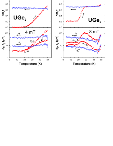
Figure 3: Calculated values of the reduced macroscopic magnetization $\langle m_{z}\rangle$ and the average ferromagnetic domain sizes with magnetic induction parallel ($d_{\uparrow}$) or antiparallel ($d_{\downarrow}$) to the applied magnetic field of 4 mT and 8 mT in UGe₂ for increasing and decreasing temperature.

For 4 mT and increasing temperature (after zero field cooling), the reduced magnetization $\langle m_{z}\rangle$ remains equal to 0 up to $T_{X}\approx 20$ K. As a consequence $d_{\downarrow}$ is equal to $d_{\uparrow}$ and of the same order of the zero field values. Above $T_{X}$ however the system gets magnetically soft and $\langle m_{z}\rangle$ starts to increase linearly towards $\sim 0.7$. Domain walls are expelled above $T_{X}$, since $d_{\uparrow}$ increases much faster than $d_{\downarrow}$. (Note the logarithmic vertical scale.) While $d_{\uparrow}$ gets of the order of $100~{}\mu$m, $d_{\downarrow}$ only reaches $25~{}\mu$m. When the domains grow in width, at a certain moment it is no longer allowed to assume $\vec{B}(\vec{r})=\mu_{0}\vec{M}(\vec{r})$, because stray fields produced by the domains have to be taken into account. The model therefore is no longer appropriate close to $T_{C}$.

Table 1: Ferromagnetic domain sizes in UGe₂ for increasing temperature after zero field cooling (ZFC) and decreasing temperature in field (FC). The sizes of the domains with magnetization parallel to the applied magnetic field is denoted by $d_{\uparrow}$ and the domains with antiparallel magnetization by $d_{\downarrow}$. Below $T_{X}$ the domain sizes are temperature independent. Above $T_{X}$ the domains grow. The values shown are at a few Kelvin below $T_{C}$.

$\mu_{0}H$	Temp.	$d_{\uparrow}$ ($\mu$m)	$d_{\downarrow}$ ($\mu$m)	$d_{\uparrow}$ ($\mu$m)	$d_{\downarrow}$ ($\mu$m)
(mT)	incr./decr.	$T<T_{X}$	$T<T_{X}$	$T\approx T_{C}$	$T\approx T_{C}$
0	ZFC, incr.	4.4(1)	4.4(1)	4.4(1)	4.4(1)
0	FC, decr.	5.1(2)	5.1(2)	5.1(2)	5.1(2)
4	ZFC, incr.	3.9(1)	3.8(1)	150(20)	25(5)
4	FC, decr.	46.4(8)	9.5(2)	60(10)	13(2)
8	ZFC, incr.	17.9(2)	11.4(1)	85(20)	10(2)
8	FC, decr.	45(5)	8.2(1)	85(20)	10(5)

For field cooling in 4 mT, the system has $\langle m_{z}\rangle=0.668(1)$ for the whole temperature range below $T_{C}$. The values of the domain size are shown in table 1.

When after zero field cooling a field of 8 mT is turned on, the sample does get a macroscopic magnetization, in contrast to the case of 4 mT. Up to $T_{X}\approx 20$ K the reduced magnetization $\langle m_{z}\rangle=0.221(2)$ is independent of temperature. Then $\langle m_{z}\rangle$ starts to increase up to 0.718(3) around 30 K and is constant afterwards up to $T_{C}$. When cooling down in 8 mT, $\langle m_{z}\rangle=0.708(1)$ over the whole temperature range below $T_{C}$.

For field warming after zero field cooling, the calculation of the domain sizes yields unexpected temperature dependencies of domain sizes above $T_{X}$. As can be seen in Fig. 3, according to the model the domain sizes grow above $T_{X}$ to decrease in size again at higher temperature. Clearly there is another source of depolarization, not accounted for by the model. Since the field is strong enough to penetrate the sample, additional depolarization arises from an inhomogeneous magnetic domain structure.

IV.2 Discussion

If the domain width becomes relatively large compared to its length, stray fields become important and the simple model assuming $\vec{B}(\vec{r})=\mu_{0}\vec{M}(\vec{r})$ is no longer valid. Calculation of the mean-square direction cosine along the $z$ direction, $\gamma_{z}$, with Eq. 10, indeed shows a decrease from unity above $T_{X}$, indicating that the magnetic induction $\vec{B}$ is not along the $\bf a$ axis throughout the sample. The model can of course be improved if we no longer assume a length/width ratio of infinity (no stray fields) for the domains. The simple model together with our measurements, however, do show that the magnetic domain sizes in zero field are a few $\mu$m and that by applying small fields the domains grow. Our measurements therefore indicate that the domain sizes in UGe₂ at ambient pressure and down to 2 K are certainly larger than the 40 Å predicted by Nishioka et al.Nishioka et al. (2002, 2003)

In Fig. 1 it is shown that $D_{zz}$ is less than unity below $T_{C}$. This can be caused by the domain walls, but can also be accounted for by a misalignment. A simple calculation shows that a misalignment of $8^{\circ}$ would fully account for the values of $D_{zz}$ below $T_{C}$. The stated value of $\delta=0.22~{}\mu$m (or $\delta/d=0.047(23)$) should therefore be regarded as an upper limit.

From the above considerations we conclude that the domain structure of UGe₂ behaves like in a conventional ferromagnet. The magnetic domain size largely exceeds the superconducting correlation length of the Cooper pair. The magnetic domain boundaries can therefore only give secondary effects on the superconducting order.

V Conclusion

The ferromagnetic domain sizes of UGe₂ was studied by means of three dimensional neutron depolarization at ambient pressure. We conclude that the existence of field-tuned resonant tunneling between spin quantum states Nishioka et al. (2002, 2003) is highly unlikely. The requirement of this model is a ferromagnetic domain size of 40 Å  while our measurements indicate a size a factor of 1000 larger. The observed jumps in the magnetization should be attributed to a Barkhausen effect as discussed by Lhotel et al. Lhotel et al. (2003). The superconductivity therefore exists within a single ferromagnetic domain. The domain walls are not expected to strongly affect the bulk Cooper pair wave function, as suggested by Nishioka et al. Nishioka et al. (2002, 2003), since the domain wall is less than a few percent of the average domain size.

Appendix A Effect of stray fields induced by a homogeneously magnetized sample

In this appendix we will calculate the magnetic induction $\vec{B}$ generated by a uniformly magnetized sample with length $l$, width $w$, and thickness $t$ (Fig. 4).

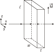
Figure 4: Schematic layout of a homogeneously magnetized rectangular sample.

Moreover, analytical expressions will be given for the line integrals of $\vec{B}$ along the path of a neutron. The center of the sample is taken as the origin of the reference frame.

Our starting point is the Biot-Savart law:

$$\vec{B}(x,y,z)=\frac{\mu_{0}}{4\pi}\int_{S}\frac{\vec{M}\times\vec{n}\times\vec{r}}{r^{3}}dS+\frac{\mu_{0}}{4\pi}\int_{\tau}\frac{\nabla\times\vec{M}\times\vec{r}}{r^{3}}d\tau$$ (14)

where $\mu_{0}=4\pi\times 10^{-7}$ H/m, $\vec{M}$ is the magnetization, $\vec{n}$ the unit vector perpendicular to the surface $S$ of the sample, $\vec{r}$ the vector pointing from the surface $S$ to the point $(x,y,z)$, and $\tau$ the volume of the sample. Since the sample has a homogeneous magnetization, the second term vanishes and, with $\vec{m}=\vec{M}/M$, we have

$$\vec{B}=\frac{\mu_{0}M}{4\pi}\int_{S}\frac{\vec{m}\times\vec{n}\times\vec{r}}{r^{3}}dS.$$ (15)

A straightforward but tedious calculation shows that

$$B_{x} = -\sum_{\epsilon_{1},\epsilon_{2},\epsilon_{3}=\pm 1}\epsilon_{1}\epsilon_{2}\epsilon_{3}\ln\left(\mathcal{S}-\left(2y+\epsilon_{2}w\right)\right)$$

$$B_{y} = -\sum_{\epsilon_{1},\epsilon_{2},\epsilon_{3}=\pm 1}\epsilon_{1}\epsilon_{2}\epsilon_{3}\ln\left(\mathcal{S}-\left(2x+\epsilon_{1}t\right)\right)$$ (16)

$$B_{z} = \sum_{\epsilon_{1},\epsilon_{2},\epsilon_{3}=\pm 1}\epsilon_{1}\epsilon_{2}\epsilon_{3}\arctan\left(\frac{2z+\epsilon_{3}l}{\left(2x+\epsilon_{1}t\right)\left(2y+\epsilon_{2}w\right)}\;\mathcal{S}\right)$$

where

$$\mathcal{S}=\sqrt{\left(2x+\epsilon_{1}t\right)^{2}+\left(2y+\epsilon_{2}w\right)^{2}+\left(2z+\epsilon_{3}l\right)^{2}}.$$ (17)

The rotation of the polarization of a neutron beam depends on the line integral of the magnetic field along the neutron path. From the Larmor equation $\frac{d}{dt}\vec{P}(t)=\gamma\vec{P}(t)\times\vec{B}(t)$, or equivalently $\frac{d}{dx}\vec{P}(x)=\left(\gamma/v\right)\vec{P}(x)\times\vec{B}(x)$ where $\gamma=1.83\times 10^{8}$ s^-1T^-1 the gyromagnetic ratio of the neutron and $v$ its velocity, we get the general solution

$$\vec{P}(x,y,z)=\left\{\exp\left(\frac{\gamma}{v}\int_{-\infty}^{x}\overline{\overline{B}}(x^{\prime},y,z)dx^{\prime}\right)\right\}\vec{P}(-\infty,y,z)$$ (18)

where we have defined the magnetic field tensor $\overline{\overline{B}}$ as

$$\overline{\overline{B}}(x,y,z)=\left(\begin{array}[]{ccc}0&B_{z}&-B_{y}\\ -B_{z}&0&B_{x}\\ B_{y}&-B_{x}&0\\ \end{array}\right)(x,y,z)$$ (19)

Thus, in order to calculate the rotation of the neutron beam polarization due to a homogeneously magnetized sample, the following line integrals are required:

$$X(y,z)=\int_{-\infty}^{\infty}B_{x}(x^{\prime},y,z)dx^{\prime}=0$$

$$Y(y,z)=\int_{-\infty}^{\infty}B_{y}(x^{\prime},y,z)dx^{\prime}=$$

$$\hskip 14.22636pt-\frac{t\mu_{0}M}{4\pi}\sum_{\epsilon_{2},\epsilon_{3}}\epsilon_{2}\epsilon_{3}\ln\left(\left(2y+\epsilon_{2}w\right)^{2}+\left(2z+\epsilon_{3}l\right)^{2}\right)$$

$$Z(y,z)=\int_{-\infty}^{\infty}B_{z}(x^{\prime},y,z)dx^{\prime}=$$

$$\hskip 14.22636pt\frac{t\mu_{0}M}{2\pi}\sum_{\epsilon_{2},\epsilon_{3}}\epsilon_{2}\epsilon_{3}\arctan\left(\frac{2z+\epsilon_{3}l}{2y+\epsilon_{2}w}\right)$$

(20)

For completeness we also give the line integrals in the case the neutron beam is along the $z$-direction:

$$X^{\prime}(x,y)=\int_{-\infty}^{\infty}B_{x}(x,y,z^{\prime})dz^{\prime}=0$$

$$Y^{\prime}(x,y)=\int_{-\infty}^{\infty}B_{y}(x,y,z^{\prime})dz^{\prime}=0$$

$$Z^{\prime}(x,y)=\int_{-\infty}^{\infty}B_{z}(x,y,z^{\prime})dz^{\prime}=\mu_{0}M\;l$$ (21)

From Eq. 18 and the above line integrals we get for the final polarization $\vec{P}(\infty,y,z)=\overline{\overline{D}}(y,z)\times\vec{P}(-\infty,y,z)$ with $\overline{\overline{D}}(y,z)$ equal to

$$\small\frac{1}{\Sigma}\!\left(\!\!\!\begin{array}[]{ccc}\Sigma\cos a\sqrt{\Sigma}&Z\sqrt{\Sigma}\sin a\sqrt{\Sigma}&-Y\sqrt{\Sigma}\sin a\sqrt{\Sigma}\\ -Z\sqrt{\Sigma}\sin a\sqrt{\Sigma}&Z^{2}\cos a\sqrt{\Sigma}+Y^{2}&YZ\left(1-\cos a\sqrt{\Sigma}\right)\\ Y\sqrt{\Sigma}\sin a\sqrt{\Sigma}&YZ\left(1-\cos a\sqrt{\Sigma}\right)&Y^{2}\cos a\sqrt{\Sigma}+Z^{2}\\ \end{array}\!\!\!\right)$$ (22)

where $\Sigma(y,z)=Y^{2}(y,z)+Z^{2}(y,z)$ and $a=\gamma/v$.

Now Eq. 22 relates the initial polarization to the final polarization for a beam passing through the sample at $(y,z)$. For a neutron beam with finite cross section the matrix $\overline{\overline{D}}$ should be integrated over the beam cross section. If the integration is symmetric relative to the origin, then we can make use of the fact that

$$B_{y}(\epsilon_{1}x,\epsilon_{2}y,\epsilon_{3}z)=\epsilon_{2}\epsilon_{3}\;B_{y}(x,y,z),$$ (23)

where $\epsilon_{1},\epsilon_{2},\epsilon_{3}=\pm 1$. This means that $B_{y}(x,y,z)$ and therefore $Y(y,z)$ are antisymmetric with respect to $y$ and $z$. Therefore, from Eq. 22, we only have to integrate the matrix

$$\small\frac{1}{\Sigma}\left(\!\!\!\begin{array}[]{ccc}\Sigma\cos a\sqrt{\Sigma}&Z\sqrt{\Sigma}\sin a\sqrt{\Sigma}&0\\ -Z\sqrt{\Sigma}\sin a\sqrt{\Sigma}&Z^{2}\cos a\sqrt{\Sigma}+Y^{2}&0\\ 0&0&Y^{2}\cos a\sqrt{\Sigma}+Z^{2}\\ \end{array}\!\!\!\right)$$ (24)

over the cross section of the neutron beam.

An infinitely narrow neutron beam passing exactly through the middle of the sample will only have its polarization rotated by $B_{z}(x,0,0)$ since $B_{x}(x,0,0)$ and $B_{y}(x,0,0)$ vanish. As long as $Y^{2}(y,z)$ is small compared to $Z^{2}(y,z)$, which is valid if $(y,z)$ is sufficiently far from the edges, Eq. 24 is a pure rotation matrix.

It is now possible to calculate the magnetization of the sample from the measured rotation angle (Eq. 8). If no stray fields were present, the rotation angle would be given by $t\mu_{0}M\gamma/v$. However, the stray fields reduce the rotation angle to $\gamma/vZ(y,z)$ with $Z(y,z)$ given in Eq. 20. We can therefore define the geometrical factor $\eta$ as

$$\phi=\eta\mu_{0}Mt\gamma/v$$ (25)

where $\eta(y,z)$ is given by

$$\eta(y,z)=\frac{1}{2\pi}\sum_{\epsilon_{2},\epsilon_{3}}\epsilon_{2}\epsilon_{3}\arctan\left(\frac{2z+\epsilon_{3}l}{2y+\epsilon_{2}w}\right).$$ (26)

Since $\eta(0,0)$ is a saddle point ($\eta(0,z)$ has a local maximum and $\eta(y,0)$ a local minimum) an average over the cross section of the neutron beam, centered around the middle of the sample, will yield a result very close to the value of $\eta(0,0)$, which is given by

$$\eta=\frac{2}{\pi}\arctan\left(\frac{l}{w}\right).$$ (27)

References

- Saxena et al. (2000) S. S. Saxena, P. Agarwal, K. Ahilan, F. M. Grosche, R. K. W. Haselwimmer, M. J. Steiner, E. Pugh, I. R. Walker, S. R. Julian, P. Monthoux, et al., Nature (London) 406, 587 (2000).
- Aoki et al. (2001) D. Aoki, A. Huxley, E. Ressouche, D. Braithwaite, J. Flouquet, J.-P. Brison, E. Lhotel, and C. Paulsen, Nature (London) 413, 613 (2001).
- Moncton et al. (1978) D. E. Moncton, G. Shirane, W. Thomlinson, M. Ishikawa, and O. Fischer, Phys. Rev. Lett. 41, 1133 (1978).
- Majkrzak et al. (1979) C. F. Majkrzak, G. Shirane, W. Thomlinson, M. Ishikawa, O. Fischer, and D. E. Moncton, Solid State Commun. 31, 773 (1979).
- Thomlinson et al. (1981) W. Thomlinson, G. Shirane, D. E. Moncton, M. Ishikawa, and O. Fischer, Phys. Rev. B 23, 4455 (1981).
- Walker et al. (1997) I. R. Walker, F. M. Grosche, D. M. Freye, and G. G. Lonzarich, Physica C 282, 303 (1997).
- Grosche et al. (1997) F. M. Grosche, S. J. S. Lister, F. V. Carter, S. S. Saxena, R. K. W. Haselwimmer, N. D. Mathur, S. R. Julian, and G. G. Lonzarich, Physica B 239, 62 (1997).
- Sato et al. (2001) N. K. Sato, N. Aso, K. Miyake, R. Shiina, P. Thalmeier, G. Varelogiannis, C. Geibel, F. Steglich, P. Fulde, and T. Komatsubara, Nature (London) 410, 340 (2001).
- Fertig et al. (1977) W. A. Fertig, D. C. Johnston, L. E. DeLong, R. W. McCallum, M. B. Maple, and B. T. Matthias, Phys. Rev. Lett. 38, 987 (1977).
- Moncton et al. (1980) D. E. Moncton, D. B. McWhan, P. H. Schmidt, G. Shirane, W. Thomlinson, M. B. Maple, H. B. MacKay, L. D. Woolf, Z. Fisk, and D. C. Johnston, Phys. Rev. Lett. 45, 2060 (1980).
- Ishikawa and Fischer (1977) M. Ishikawa and O. Fischer, Solid State Commun. 23, 37 (1977).
- Tateiwa et al. (2001) N. Tateiwa, T. C. Kobayashi, K. Hanazono, K. Amaya, Y. Haga, R. Settai, and Y. Onuki, J. Phys. Condens. Matter 13, L17 (2001).
- Nishioka et al. (2002) T. Nishioka, G. Motoyama, S. Nakamura, H. Kadoya, and N. K. Sato, Phys. Rev. Lett. 88, 237203 (2002).
- Nishioka et al. (2003) T. Nishioka, N. K. Sato, and G. Motoyama, Phys. Rev. Lett. 91, 209702 (2003).
- Boulet et al. (1997) P. Boulet, A. Daoudi, M. Potel, H. Noel, G. M. Gross, G. Andre, and F. Bouree, J. Alloys Comp. 247, 104 (1997).
- Onuki et al. (1992) Y. Onuki, I. Ukon, S. W. Yun, I. Umehara, K. Satoh, T. Fukuhara, H. Sato, S. Takayanagi, M. Shikama, and A. Ochiai, J. Phys. Soc. Jpn. 61, 293 (1992).
- Huxley et al. (2000) A. Huxley, I. Sheikin, and D. Braithwaite, Physica B 284-288, 1277 (2000).
- Rekveldt (1973) M. T. Rekveldt, Z. Phys. 259, 391 (1973).
- Rosman and Rekveldt (1990) R. Rosman and M. T. Rekveldt, Z. Phys. B 79, 61 (1990).
- Rosman and Rekveldt (1991) R. Rosman and M. T. Rekveldt, Phys. Rev. B 43, 8437 (1991).
- Pfleiderer and Huxley (2002) C. Pfleiderer and A. D. Huxley, Phys. Rev. Lett. 89, 147005 (2002).
- Lhotel et al. (2003) E. Lhotel, C. Paulsen, and A. D. Huxley, Phys. Rev. Lett. 91, 209701 (2003).