Lattice density functional for colloid-polymer mixtures:
Multi-occupancy versus Highlander version

Abstract

We consider a binary mixture of colloid and polymer particles with positions on a simple cubic lattice. Colloids exclude both colloids and polymers from nearest neighbor sites. Polymers are treated as effective particles that are mutually non-interacting, but exclude colloids from neighboring sites; this is a discrete version of the (continuum) Asakura-Oosawa-Vrij model. Two alternative density functionals are proposed and compared in detail. The first is based on multi-occupancy in the zero-dimensional limit of the bare model, analogous to the corresponding continuum theory that reproduces the bulk fluid free energy of free volume theory. The second is based on mapping the polymers onto a multicomponent mixture of polymer clusters that are shown to behave as hard cores; the corresponding (Highlander) property of the extended model in strong confinement permits direct treatment with lattice fundamental measure theory. Both theories predict the same topology for the phase diagram with a continuous fluid-fcc freezing transition at low polymer fugacity and, upon crossing a tricritical point, a first-order freezing transition for high polymer fugacities with rapidly broadening density jump.

I Introduction

Mixtures of colloidal particles and non-adsorbing polymers suspended in a common solvent Poon (2002); Tuinier et al. (2003) have been theoretically investigated on various levels of description, ranging from simplistic to realistic effective interactions between the constituent particles. The prototype of the former is the Asakura-Oosawa-Vrij (AOV) model Asakura and Oosawa (1954); Vrij (1976) that describes the colloids as hard spheres and the polymers as ideal (i.e., non-interacting) effective spheres that interact via hard core repulsion with the colloids. Despite its simplicity this model reproduces the essential trends in bulk phase behavior of colloid-polymer mixtures, involving colloidal gas, liquid, and crystalline phases Lekkerkerker et al. (1992); Meijer and Frenkel (1994); Dijkstra et al. (1999); P. G. Bolhuis, A. A. Louis, J. P. Hansen (2002), and proved to be useful for studying a range of interfacial properties Brader et al. (2003), like the structure of colloidal gas-liquid interfaces and wetting of substrates, issues that are experimentally relevant Aarts et al. (2003); Aarts and Lekkerkerker (2004); Wijting et al. (2003).

Density functional theory Evans (1979, 1992) is a primary tool to treat spatially inhomogeneous systems. For the common reference model of additive mixtures of hard spheres, the fundamental measures theory (FMT) Rosenfeld (1989) is many investigators’ current choice. This approach was extended to cover the AOV model Schmidt et al. (2000), thereby triggering much further interest in the study of interfacial properties of this model, see e.g. Schmidt et al. (2004) for recent work on novel effects in sedimentation-diffusion equilibrium. In a different direction, FMT was recently generalized to hard core lattice models Lafuente and Cuesta (2002, 2003, 2004) elucidating the very foundation of the FMT approach.

Despite its usefulness for practical applications, the AOV functional of Ref. Schmidt et al. (2000) possesses several deficiencies, that are absent in the hard sphere FMT (see Ref. Schmidt et al. (2002) for a detailed discussion): i) When applied to one spatial dimension a spurious phase transition is predicted Schmidt et al. (2002), that is absent (as befits a model with short-ranged interactions) in the exact solution Brader and Evans (2002). ii) In three dimensions the location of the bulk fluid-fluid critical point lies at lower polymer fugacity as compared to the value obtained with simulations. iii) The excess free energy is a linear functional of the polymer density profile.

While we will not present a full resolution of the above issues, dealing with a lattice model allows us to go significant steps beyond the recipe of construction of Ref. Schmidt et al. (2000). Hence we consider a simplified version of the AOV model by constraining the position coordinates to an underlying lattice, for convenience taken to be of simple cubic symmetry. We are inspired by the fact that similar lattice models have been proven useful in soft matter research to make qualitative predictions, like e.g. for demixing Widom (1967); Frenkel and Louis (1992) and three-phase equilibria van Duijneveldt and Lekkerkerker (1993). Also much vital attention has been recently paid to lattice models with short-ranged attractive interactions to address adsorption in disordered porous media Kierlik et al. (2001, 2002); Sarkisov and Monson (2002); Detcheverry et al. (2003); Woo and Monson (2003).

We consider the case of small particles sizes, namely such that particles only repel other particles from nearest neighbor sites. As the polymers are ideal, each site may be occupied by more than one of those particles. We compare two different DFTs for the binary AOV lattice model, both based on the lattice fundamental measure theory (LFMT) Lafuente and Cuesta (2002, 2003, 2004). The first approach allows for multi-occupancy of polymers in the zero-dimensional limit, and hence constitutes the lattice version of the (continuum) theory of Ref. Schmidt et al. (2000). The second approach relies on the introduction of polymer clusters as quasi-species that feature hard-core interactions only. We hence arrive at an extended model that possesses a “Highlander” onl property: In an appropriately small cavity, there can only be one particle. Exploiting further the fact that LFMT can cope directly with small non-additivities Lafuente and Cuesta (2002), we arrive at a theory for the AOV model that is exact when applied to one dimension; hence it does correctly predict the absence of phase transitions. We find that although the derivations of the two DFTs, as well as their appearance at first glance differ markedly, the results for bulk phase behavior in three dimensions are very similar, demonstrating the internal consistency of FMT.

The paper is organized as follows. In Sec. II we define the lattice AOV model. Sec. III is devoted to the construction of both density functional theories. In Sec. IV results for the bulk phase diagram are presented and we conclude in Sec. V.

II The model

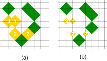
Figure 1: (a) Illustration of the lattice AOV model realized in $d=2$ spatial dimensions. Colloidal particles (dark rhombi) exclude their site and their nearest neighbor sites to colloids and polymers. Polymer particles (light rhombi) exclude colloids from their site and their nearest neighbor sites, but can overlap freely with other polymers. Integers indicate the number of (overlapping) polymers at occupied sites. (b) Equivalent non-additive multi-component hard core mixture. Clusters of overlapping polymers in (a) are viewed as quasi-particles (light rhombi) that exclude their site to other polymer clusters, and their site and their nearest neighbor sites to colloids. Integers enumerate the different species of polymer clusters and correspond to the number of overlapping polymers on the lattice sites in (a). Colloids (dark rhombi) behave as in (a).

We consider a binary mixture of particles representing colloids (species $c$) and polymers (species $p$) on the $d$-dimensional simple cubic lattice $\mathbb{Z}^{d}$. The interaction between colloids is that of site-exclusion and nearest neighbor exclusion, corresponding to the pair interaction potential

$$V_{cc}({\bf r})=\begin{cases}\infty&\mbox{if $|{\bf r}|\leq 1$,}\\ 0&{\rm otherwise,}\end{cases}$$ (1)

where ${\bf r}\in\mathbb{Z}^{d}$ is the center-center distance between the particles. Colloids and polymers interact similarly:

$$V_{cp}({\bf r})=\begin{cases}\infty&\mbox{if $|{\bf r}|\leq 1$,}\\ 0&{\rm otherwise,}\end{cases}$$ (2)

while polymers are ideal (non-interacting),

$$V_{pp}({\bf r})=0.$$ (3)

In essence this is a discretized AOV model with equal-sized components; see Fig. 1a for a sketch.

III Density functional theories

III.1 Overview of LFMT

As is customary in density functional theory Evans (1979, 1992), we express the Helmholtz free energy functional as $F=F_{\rm id}+F_{\rm ex}$, where the free energy of the binary ideal lattice gas is

$$F_{\rm id}[\rho_{c},\rho_{p}]=\sum_{i=c,p}\sum_{{\bf r}\in\mathcal{L}}\rho_{i}({\bf r})[\ln(\rho_{i}({\bf r}))-1],$$ (4)

with $\rho_{i}({\bf r})$ being the occupancy probability of site ${\bf r}$ by particles of species $i=c,p$, and $\mathcal{L}$ denoting the lattice, here $\mathcal{L}=\mathbb{Z}^{d}$. For the excess contribution to the total free energy, $F_{\rm ex}$, we will in the following use two different implementations of LFMT. This theory permits to obtain an approximation to $F_{\rm ex}$ for a lattice model from the exact solution obtained in finite (and small) sets of lattice sites, alternatively called nodes Lafuente and Cuesta (2002, 2003, 2004). The essential step determining the accuracy of the theory is the choice of maximal cavities Lafuente and Cuesta (2004). Those are maximal in the sense that any further cavity taken into consideration can be obtained as an intersection of maximal cavities. The common choice (inherited from the continuum version of the theory Rosenfeld et al. (1996); Tarazona and Rosenfeld (1997); Tarazona (2000)) for these maximal cavities is to set them equal to zero-dimensional (0d) cavities, as detailed below. Once chosen, the cavities uniquely determine the form of the functional under the requirement that it yields the exact result when evaluated at 0d density profiles Lafuente and Cuesta (2004). For a general binary mixture (with species labeled by $c$ and $p$) the final result possesses the form

$$F_{\rm ex}[\rho_{c},\rho_{p}]=\sum_{{\cal C}\,\rm cavities}a(\mathcal{C})F_{\rm ex}^{\mathcal{C}}[\rho_{c},\rho_{p}],$$ (5)

where the summation runs over the set of maximal cavities and their nonempty intersections; the $a(\mathcal{C})$ are uniquely determined integer coefficients Lafuente and Cuesta (2004), and $F_{\rm ex}^{\mathcal{C}}$ is the exact excess free energy functional of the system when confined to cavity $\mathcal{C}$.

III.2 Multi-occupancy version of DFT

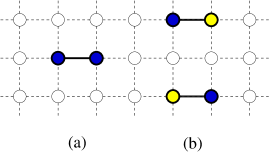
Figure 2: Maximal cavities along the X axis (the ones along the Y axis are just 90^∘ rotations of these ones) for the multi-occupancy (a) and the Highlander (b) DFTs. Dark nodes can be occupied either by colloidal or by polymer particles; light nodes can only be occupied by colloidal particles.

The definition of 0d cavities for lattice models with only hard-core interactions is unambiguous: Any set of nodes that can accommodate at most one particle constitutes a 0d cavity. For the present model, however, this is problematic: As polymers are ideal, even a single lattice site can be multiply occupied by polymers, hence no 0d cavity can contain polymers, and the resulting functional would account for them only through the ideal part, entirely ignoring the colloid-polymer interaction. One way out is to relax the definition: Any set of nodes in which any two particles present necessarily overlap constitutes a 0d cavity Schmidt et al. (2000). Hence, as opposed to the first definition, the presence of more than one particle is not excluded a priori. (For mixtures with only hard core interactions, both definitions are equivalent.)

For the present model it is straightforward to show that according to the modified (multi-occupancy) definition, any pair of adjacent nodes on the simple cubic lattice constitutes a maximal 0d cavity (Fig. 2a): Such an arrangement can either hold one colloid or an arbitrary number of (overlapping) polymers. Adding an additional node destroys the 0d character as (at least) two nonoverlapping particles will fit. Implementing the scheme of Ref. Lafuente and Cuesta, 2004 with this choice of basic cavities we obtain

$$\beta F_{\rm ex}[\rho_{c},\rho_{p}]=\sum_{{\bf r}}\Phi({\bf r}),$$ (6)

with $\beta=1/(k_{B}T)$, where $T$ is temperature and $k_{B}$ is the Boltzmann constant, and the (scaled) free energy density is

$$\begin{split}\Phi({\bf r})=&\left[\sum_{\alpha=1}^{d}\phi^{\rm AOV}_{0}\Big{(}n^{(\alpha)}_{c}({\bf r}),n^{(\alpha)}_{p}({\bf r})\Big{)}\right]\\ &-(2d-1)\phi^{\rm AOV}_{0}\Big{(}\rho_{c}({\bf r}),\rho_{p}({\bf r})\Big{)},\end{split}$$ (7)

depending on weighted densities

$$n^{(\alpha)}_{i}({\bf r})\equiv\,\rho_{i}({\bf r})+\rho_{i}({\bf r}+{\bf e}_{\alpha}),\qquad i=c,p,$$ (8)

where ${\bf e}_{\alpha}$ denotes the unit Cartesian vector along the $\alpha=1,\ldots,d$ axis and

$$\phi^{\rm AOV}_{0}(\eta_{c},\eta_{p})=(1-\eta_{c}-\eta_{p})\ln(1-\eta_{c})+\eta_{c}$$ (9)

is the excess free energy of a 0d cavity for the AOV model Schmidt et al. (2000); we give a derivation of $\phi^{\rm AOV}_{0}(\eta_{c},\eta_{p})$ in the Appendix. Since $\phi^{\rm AOV}_{0}(\eta_{c},\eta_{p})$ depends linearly on $\eta_{p}$ as

$$\phi^{\rm AOV}_{0}(\eta_{c},\eta_{p})=\phi_{0}(\eta_{c})+\eta_{p}\phi^{\prime}_{0}(\eta_{c}),$$ (10)

where

$$\phi_{0}(\eta)\equiv\eta+(1-\eta)\ln(1-\eta),$$ (11)

(7) admits the rewriting

$$\begin{split}\Phi=&\left[\sum_{\alpha=1}^{d}\phi_{0}(n^{(\alpha)}_{c})\right]-(2d-1)\phi_{0}(\rho_{c})\\ &-\rho_{p}\ln\left(\frac{\prod_{\alpha=1}^{d}(1-n^{(\alpha)}_{c})(1-\bar{n}^{(\alpha)}_{c})}{(1-\rho_{c})^{2d-1}}\right),\end{split}$$ (12)

where, for the sake of notational simplicity, we omit here and in the following the dependence of $\rho_{c},\rho_{p},n_{c}^{(\alpha)}$ on ${\bf r}$ and have introduced the short-hand notation $\bar{n}_{c}^{(\alpha)}\equiv n_{c}^{(\alpha)}({\bf r}-{\bf e}_{\alpha})$.

The linear dependence of the functional on $\rho_{p}({\bf r})$ yields a particularly simple form of the Euler-Lagrange equation for the polymer density distribution,

$$\rho_{p}=z_{p}\frac{\prod_{\alpha=1}^{d}(1-n^{(\alpha)}_{c})(1-\bar{n}^{(\alpha)}_{c})}{(1-\rho_{c})^{2d-1}},$$ (13)

being explicit in $\rho_{p}$ (i.e., independent on the right hand side of $\rho_{p}$). Given that we have eliminated $\rho_{p}({\bf r})$ as a functional of $\rho_{c}({\bf r})$, $\rho_{c}({\bf r}\pm{\bf e}_{\alpha})$, $\alpha=1,\dots,d$, and $z_{p}({\bf r})$, the Legendre-transformed functional $\beta\Upsilon_{\rm ex}[\rho_{c},z_{p}]=\sum_{{\bf r}}\Phi^{\rm eff}({\bf r})$, with

$$\Phi^{\rm eff}=\rho_{p}\ln(\rho_{p}/z_{p})-\rho_{p}+\Phi,$$ (14)

is an excess free energy functional for the effective one-component fluid of colloidal particles interacting through polymer depletion; $\rho_{p}({\bf r})$ is obtained from (13). The strength of the depletion interaction is controlled by $z_{p}({\bf r})$, which in turn can be determined by an external potential acting on the polymers and by the polymer fugacity. (A more detailed account of the procedure to obtain functionals for effective fluids can be found in Ref. Cuesta and Martínez-Ratón, 1999.) With the appropriate substitutions, we obtain

$$\begin{split}\Phi^{\rm eff}&=\left[\sum_{\alpha=1}^{d}\phi_{0}(n^{(\alpha)}_{c})\right]-(2d-1)\phi_{0}(\rho_{c})\\ &-z_{p}\frac{\prod_{\alpha=1}^{d}(1-n^{(\alpha)}_{c})(1-\bar{n}^{(\alpha)}_{c})}{(1-\rho_{c})^{2d-1}}.\end{split}$$ (15)

This completes the prescription for the lattice analog of the continuum AOV functional of Ref. Schmidt et al. (2000).

III.3 Highlander version of DFT

III.3.1 Strategy of polymer clusters as quasi-particles

Here we elude the presence of several particles inside a cavity and aim at sticking to the stronger (Highlander) definition: There can be only one onl (here: particle in the cavity). For this purpose, polymer ideality constitutes a major problem, as in the AOV lattice model each site occupied by a polymer can be occupied simultaneously by an arbitrary number of further polymers. To circumvent this problem we will hence map the model onto an extended one: We refer to a piling of $n$ polymers at the same node as a “polymer cluster” and treat polymer clusters as quasi-particles of a set of new species labeled by $n$. Thus there is a one-to-one correspondence between each configuration of polymers of the original model and a corresponding (unique) configuration of polymer clusters of the new model. (Colloids are treated as before.) We regard polymer clusters as having shapes smaller than the original polymer, see Fig. 1b. As a consequence, polymer clusters behave as hard core particles with i) site exclusion to other polymer clusters and ii) site exclusion and nearest neighbor exclusion to colloids. Clearly, feature ii) is directly inherited from the colloid-polymer interaction. Feature i) may be unexpected at first glance. Consider that a site occupied by an $n$-polymer cluster cannot be simultaneously occupied by an $m$-polymer cluster. Although in the original model the site can well be occupied by $m+n$ polymers, in the extended model such a configuration corresponds to one single $(m+n)$-polymer cluster. Hence polymer clusters repel like hard cores do.

Despite being nonadditive, the new model belongs to a class of nonadditive lattice models which are amenable to LFMT and whose one-dimensional version was shown to be exact Lafuente and Cuesta (2002). The 0d cavities for the new model are nontrivial and consist of two adjacent nodes available for the colloids, one of which (but only one) is also available to a quasi-particle (polymer cluster) of any species (Fig. 2b). Clearly, the presence of either one colloidal particle or one quasi-particle excludes other particles from the cavity, and such cavities are obviously maximal.

Here we will construct the corresponding free energy functional in two steps. First, for simplicity, we consider the quasi-particle model with a single quasi-particle species, $n=1$. Second, we will handle the full (infinite) number of quasi-particle species. Subsequently mapping the result back yields a DFT for the lattice AOV model.

III.3.2 Binary mixture with one quasi-species

For the binary mixture of colloids and $1$-polymer clusters, with density fields $\rho_{c}({\bf r})$ and $\rho_{1}({\bf r})$, respectively, according to Refs. Lafuente and Cuesta, 2002, 2004, the excess free energy density $\Phi({\bf r})$ is given by

$$\Phi({\bf r}) = \sum_{i=1}^{d}\left\{\phi_{0}\left(n_{c}^{(\alpha)}({\bf r})+\rho_{1}({\bf r})\right)\right.$$ (16)

$$\left.+\phi_{0}\left(n_{c}^{(\alpha)}({\bf r}-{\bf e}_{\alpha})+\rho_{1}({\bf r})\right)-\phi_{0}\left(n_{c}^{(\alpha)}({\bf r})\right)\right\}$$

$$-(2d-1)\phi_{0}\Big{(}\rho_{c}({\bf r})+\rho_{1}({\bf r})\Big{)},$$

with $\phi_{0}(\eta)$ defined in Eq. (11). Thus, given a local fugacity field $z_{1}({\bf r})$, the Euler-Lagrange equation for the 1-polymer cluster density is

$$\rho_{1}=z_{1}\frac{\prod_{\alpha=1}^{d}(1-n_{c}^{(\alpha)}-\rho_{1})(1-\bar{n}_{c}^{(\alpha)}-\rho_{1})}{(1-\rho_{c}-\rho_{1})^{2d-1}}.$$ (17)

where again the dependence on ${\bf r}$ has been omitted. Eq. (17) is an implicit algebraic equation for $\rho_{1}({\bf r})$, so it determines $\rho_{1}({\bf r})$ as a functional of $\rho_{c}({\bf r})$ and $z_{1}({\bf r})$. This permits to obtain, as in the previous case, a functional $\beta\Upsilon_{\rm ex}[\rho_{c},z_{1}]$ for the effective one-component fluid.

III.3.3 Mixture with an infinite number of quasi-species

Incorporating the infinite number of quasi-species amounts to first correctly modifying the ideal free energy functional to $\beta F_{\rm id}[\rho_{c},\{\rho_{n}\}]=\sum_{{\bf r}}\Phi_{\rm id}({\bf r})$, with

$$\begin{split}\Phi_{\rm id}({\bf r})=&\,\rho_{c}({\bf r})\ln(\rho_{c}({\bf r}))-\rho_{c}({\bf r})\\ &+\sum_{n=1}^{\infty}\Big{[}\rho_{n}({\bf r})\ln\Big{(}{\cal V}_{n}\rho_{n}({\bf r})\Big{)}-\rho_{n}({\bf r})\Big{]},\end{split}$$ (18)

where $\rho_{n}({\bf r})$ denotes the density profile of the quasi-species of $n$-polymer clusters, and ${\cal V}_{n}$ a thermal “volume” accounting for the internal partition function of the polymers inside the cluster. (It is not hard to guess that $\mathcal{V}_{n}=n!$; nevertheless, this result will emerge explicitly from the subsequent analysis.) Secondly, we use again LFMT for the excess part of the free energy. The necessary modification over the binary case (Sec. III.3.2) in order to include the infinite number of quasi-species is actually very simple Lafuente and Cuesta (2002): we replace $\rho_{1}({\bf r})$ in (16) by the total density of polymer clusters (pc),

$$\rho_{\rm pc}({\bf r})\equiv\sum_{n=1}^{\infty}\rho_{n}({\bf r}).$$ (19)

As our aim is to describe the lattice AOV model, we have to “project” the quasi-species back to polymers. Clearly, the total cluster density and the polymer density are related via

$$\rho_{p}({\bf r})=\sum_{n=1}^{\infty}n\rho_{n}({\bf r}).$$ (20)

For convenience we will again resort to an effective one-component description. Hence we transform to the semi-grand potential

$$\beta\Upsilon[\rho_{c},z_{p}]=\min_{\{\rho_{n}\}}\sum_{{\bf r}}\Big{(}\Phi_{\rm id}({\bf r})+\Phi({\bf r})-\rho_{p}({\bf r})\ln z_{p}({\bf r})\Big{)},$$ (21)

where $\Phi_{\rm id}({\bf r})$ is given by (18), and $\Phi({\bf r})$ by (16) with $\rho_{1}({\bf r})$ replaced by $\rho_{\rm pc}({\bf r})$. With the same notation as in (17), performing the minimization in (21) yields

$$\rho_{n}=\frac{z_{p}^{n}}{\mathcal{V}_{n}}\frac{\prod_{\alpha=1}^{d}(1-n_{c}^{(\alpha)}-\rho_{\rm pc})(1-\bar{n}_{c}^{(\alpha)}-\rho_{\rm pc})}{(1-\rho_{c}-\rho_{\rm pc})^{2d-1}},$$ (22)

which using (19) leads to

$$\rho_{\rm pc}=\zeta(z_{p})\frac{\prod_{\alpha=1}^{d}(1-n_{c}^{(\alpha)}-\rho_{\rm pc})(1-\bar{n}_{c}^{(\alpha)}-\rho_{\rm pc})}{(1-\rho_{c}-\rho_{\rm pc})^{2d-1}},$$ (23)

with $\zeta(z_{p})\equiv\sum_{n=1}^{\infty}(z_{p}^{n}/\mathcal{V}_{n})$. Also, from Eqs. (20), (22) and (23) we get

$$\rho_{p}=z_{p}\frac{\zeta^{\prime}(z_{p})}{\zeta(z_{p})}\rho_{\rm pc},$$ (24)

establishing a simple proportionality between $\rho_{p}({\bf r})$ and $\rho_{\rm pc}({\bf r})$.

The function $\zeta(z_{p})$ can be easily obtained realizing that it is independent of all densities appearing in (23), rather it depends solely on $z_{p}({\bf r})$. Thus if we particularize (23), e.g. for $\rho_{c}({\bf r})=0$, we obtain the simple relationship

$$\rho_{\rm pc}=\zeta(z_{p})(1-\rho_{\rm pc}),$$ (25)

from which

$$\rho_{\rm pc}=\frac{\zeta(z_{p})}{1+\zeta(z_{p})}.$$ (26)

Then, according to Eq. (24),

$$\rho_{p}=z_{p}\frac{\zeta^{\prime}(z_{p})}{1+\zeta(z_{p})}=z_{p}\Big{(}\ln(1+\zeta)\Big{)}^{\prime},$$ (27)

and since in the absence of colloidal particles, the polymers form an ideal gas (hence $\rho_{p}=z_{p}$), we get

$$\Big{(}\ln(1+\zeta)\Big{)}^{\prime}=1.$$ (28)

The solution to this equation satisfying $\zeta(0)=0$ is

$$\zeta(z_{p})=e^{z_{p}}-1=\sum_{n=1}^{\infty}\frac{z^{n}}{n!},$$ (29)

providing the confirmation of the relationship $\mathcal{V}_{n}=n!$.

III.3.4 Functional for the lattice AOV model

Returning to Eq. (23), we observe that this equation for $\rho_{\rm pc}({\bf r})$ is formally equivalent to Eq. (17) for $\rho_{1}({\bf r})$ with $z_{1}({\bf r})$ replaced by the $\zeta\big{(}z_{p}({\bf r})\big{)}$ given by (29). Recalling the origin of Eq. (17), this means that we can describe the original AOV model in terms of the free energy functional $\beta F[\rho_{c},\rho_{\rm pc}]=\sum_{{\bf r}}\left\{\Phi_{\rm id}({\bf r})+\Phi({\bf r})\right\}$, with

$$\Phi_{\rm id} = \rho_{c}(\ln\rho_{c}-1)+\rho_{\rm pc}(\ln\rho_{\rm pc}-1)$$

$$\Phi = \sum_{i=1}^{d}\left[\phi_{0}(n_{c}^{(\alpha)}+\rho_{\rm pc})+\phi_{0}(\bar{n}_{c}^{(\alpha)}+\rho_{\rm pc})\right.$$ (30)

$$-\left.\phi_{0}(n_{c}^{(\alpha)})\right]-(2d-1)\phi_{0}(\rho_{c}+\rho_{\rm pc}),$$

with the fugacity for the total density of polymer clusters, $\rho_{\rm pc}({\bf r})$, given by

$$\zeta({\bf r})=e^{z_{p}({\bf r})}-1,$$ (31)

and the polymer density obtained from $\rho_{\rm pc}({\bf r})$ as

$$\rho_{p}({\bf r})=\frac{z_{p}({\bf r})}{1-e^{-z_{p}({\bf r})}}\,\rho_{\rm pc}({\bf r}).$$ (32)

This completes the prescription of the Highlander functional for the AOV model.

As a final note, we can alternatively obtain the effective functional $\beta\Upsilon_{\rm ex}[\rho_{c},z_{p}]=\sum_{{\bf r}}\Phi^{\rm eff}({\bf r})$, which, after a few algebraic manipulations, can be written as

$$\begin{split}\Phi^{\rm eff}=&\,\rho_{c}\ln\rho_{c}-(2d-1)(1-\rho_{c})\ln(1-\rho_{c}-\rho_{\rm pc})\\ &+\sum_{\alpha=1}^{d}\big{[}(1-n_{c}^{\alpha})\ln(1-n_{c}^{\alpha}-\rho_{\rm pc})\\ &+(1-\bar{n}_{c}^{\alpha})\ln(1-\bar{n}_{c}^{\alpha}-\rho_{\rm pc})\\ &-(1-n_{c}^{\alpha})\ln(1-n_{c}^{\alpha})\big{]},\end{split}$$ (33)

with $\rho_{\rm pc}({\bf r})$ being the solution of (23).

III.4 Relationship between both DFTs

Assuming small polymer fugacity, $z_{p}({\bf r})\ll 1$, for the Highlander DFT, from Eqs. (31) and (32) it follows that $\zeta({\bf r})\approx z_{p}({\bf r})$ and $\rho_{\rm pc}({\bf r})\approx\rho_{p}({\bf r})$. The functional is then approximately given by Eq. (16). On the other hand, small fugacities imply small densities, so we can expand (16) to linear order in $\rho_{p}({\bf r})$. Doing so and taking into account that the sum over ${\bf r}$ allows us to shift the arguments of the functions, we realize that the expansion is precisely functional (7). So both DFTs coincide at low polymer fugacities.

IV Results

As an application we consider the bulk phase diagram for the lattice AOV model and compare the predictions from both DFTs. Guided by its continuum counterpart, we expect the phase behavior of the lattice model to be determined by the interplay of hard core colloid-colloid repulsion and the (short-ranged) colloid-colloid attraction induced by polymer depletion. Thus a clear framework to study the model is the effective one-component description, cf. Eqs. (15) and (33). As in other (one-component) models with hard core repulsion and short-range attraction, both condensation (corresponding to demixing from the viewpoint of the binary mixture) and freezing may occur. We can study the former via a convexity analysis of the effective (semi-grand) free energy of a uniform fluid, and the latter by considering spatially inhomogeneous density distributions characteristic for crystalline states. Here the candidate is a face-centered cubic (fcc) structure that constitutes the close packed state for the colloids. In the following we will carry out this program for either DFT.

IV.1 Thermodynamics from the multi-occupancy DFT

As an appropriate thermodynamic potential we consider a (scaled) semi-grand free energy per volume, $Y\equiv\rho_{c}[\ln(\rho_{c})-1]+\beta\Upsilon_{\rm ex}/V$. For a uniform fluid at given polymer fugacity $z_{p}$, according to (15) this is given by

$$\begin{split}Y=&\,\frac{\eta_{c}}{2}\ln\left(\frac{\eta_{c}}{2}\right)+d(1-\eta_{c})\ln(1-\eta_{c})\\ &-(2d-1)\left(1-\frac{\eta_{c}}{2}\right)\ln\left(1-\frac{\eta_{c}}{2}\right)\\ &-z_{p}\frac{(1-\eta_{c})^{2d}}{\left[1-(\eta_{c}/2)\right]^{2d-1}},\end{split}$$ (34)

where $\eta_{c}=2\rho_{c}$ is the colloid packing fraction. Convexity implies $Y^{\prime\prime}(\eta_{c})>0$, so the spinodal condition, $Y^{\prime\prime}(\eta_{c})=0$, yields

$$\eta^{r,{\rm spin}}_{p}(\eta_{c})=\frac{2\left(1-\frac{\eta_{c}}{2}\right)^{2d}[1+(d-1)\eta_{c}]}{d(2d-1)\eta_{c}(1-\eta_{c})^{2d-1}},$$ (35)

where we have used the polymer reservoir packing fraction, $\eta^{\rm r}_{p}=2z_{p}$, as an alternative thermodynamic variable. The minimum of this curve determines the critical point, given by one of the roots of the cubic polynomial

$$(d-1)(\eta_{c}^{\rm crit})^{3}+2(d-1)^{2}(\eta_{c}^{\rm crit})^{2}+(2d+1)\eta_{c}^{\rm crit}-2=0,$$ (36)

and the corresponding value $\eta_{p}^{r,{\rm crit}}$ obtained from (35). For $d=3$ the critical point is at $\eta_{c}^{\rm crit}=\sqrt{3/2}-1\approx 0.225$ (see Fig 3). The liquid-gas binodal can be obtained from (34) via a double tangent construction, in practice carried out numerically.

For crystals we are guided by the close-packed state of the colloids, and distinguish two fcc sublattices of the underlying simple cubic lattice, each formed by the nearest neighbor nodes of the other. The colloid density at nodes of sublattices $a$ and $b$ are denoted by $\rho_{a}$ and $\rho_{b}$, respectively. Hence the average colloid packing fraction is

$$\eta_{c}=\rho_{a}+\rho_{b}.$$ (37)

The semi-grand potential is given by

$$\begin{split}Y=&\,\frac{\rho_{a}}{2}\ln\rho_{a}+\frac{\rho_{b}}{2}\ln\rho_{b}+d(1-\eta_{c})\ln(1-\eta_{c})\\ &-\left(d-{\textstyle\frac{1}{2}}\right)(1-\rho_{a})\ln(1-\rho_{a})\\ &-\left(d-{\textstyle\frac{1}{2}}\right)(1-\rho_{b})\ln(1-\rho_{b})\\ &-\frac{z_{p}}{2}\left[\frac{(1-\eta_{c})^{2d}}{(1-\rho_{a})^{2d-1}}+\frac{(1-\eta_{c})^{2d}}{(1-\rho_{b})^{2d-1}}\right].\end{split}$$ (38)

The equilibrium density distribution for given values of $\eta_{c}$ can be obtained by minimizing $Y$ with respect to $\rho_{a}$ and $\rho_{b}$ under the constraint (37), leading to the condition

$$\begin{split}\rho_{a}&(1-\rho_{a})^{2d-1}\exp\left(-(2d-1)z_{p}\left(\frac{1-\eta_{c}}{1-\rho_{a}}\right)^{2d}\right)\\ &=\rho_{b}(1-\rho_{b})^{2d-1}\exp\left(-(2d-1)z_{p}\left(\frac{1-\eta_{c}}{1-\rho_{b}}\right)^{2d}\right).\end{split}$$ (39)

This equation possesses one solution characteristic for fluid states, $\rho_{a}=\rho_{b}=\eta_{c}/2$, which is locally stable as long as it minimizes $Y(\rho_{a},\rho_{b})$, i.e. up to the value of $\eta_{c}$ at which

$$\frac{\partial^{2}}{\partial\rho_{a}^{2}}Y(\rho_{a},\eta_{c}-\rho_{a})\bigg{|}_{\rho_{a}=\eta_{c}/2}=0,$$ (40)

defining the freezing spinodal, that we can explicitly obtain as

$$\eta^{\rm r,fr}_{p}(\eta_{c})=\frac{2\left(1-\frac{\eta_{c}}{2}\right)^{d}(1-d\eta_{c})}{d(2d-1)\eta_{c}(1-\eta_{c})^{2d}}.$$ (41)

If freezing is second order, Eq. (41) directly gives the transition line in the phase diagram. In the case of a first-order transition again a numerical double tangent construction is required to obtain the coexistence densities.

IV.2 Thermodynamics from the Highlander DFT

In the fluid phase we obtain the semi-grand potential

$$\begin{split}Y=&\,\frac{\eta_{c}}{2}\ln\left(\frac{\eta_{c}}{2}\right)-(2d-1)\left(1-\frac{\eta_{c}}{2}\right)\ln\left(1-\frac{\eta_{c}}{2}-\rho_{\rm pc}\right)\\ &+d(1-\eta_{c})\ln\left(\frac{(1-\eta_{c}-\rho_{\rm pc})^{2}}{1-\eta_{c}}\right),\end{split}$$ (42)

with $\rho_{\rm pc}$ being the solution of

$$\left(1-\frac{\eta_{c}}{2}-\rho_{\rm pc}\right)^{2d-1}\rho_{\rm pc}=\zeta(z_{p})(1-\eta_{c}-\rho_{\rm pc})^{2d}.$$ (43)

Again, the fluid-fluid spinodal can be determined by $Y^{\prime\prime}(\eta_{c})=0$; necessary expressions for $\rho_{\rm pc}^{\prime}(\eta_{c})$ and $\rho_{\rm pc}^{\prime\prime}(\eta_{c})$ can be obtained implicitly from (43). The spinodal polymer cluster density is

$$\rho_{\rm pc}^{{\rm spin}}(\eta_{c})=\frac{(1-\eta_{c})\big{[}1+(d-1)\eta_{c}\big{]}}{1+(d-1)(2d+1)\eta_{c}},$$ (44)

which inserted into (43) gives the liquid-gas spinodal

$$\begin{split}\eta_{p}^{\rm r,spin}(\eta_{c})=&\,2\ln\Bigg{(}1+\frac{2(2d-1)^{2d-1}}{\big{[}4d(d-1)\big{]}^{2d}}\big{[}1+(d-1)\eta_{c}\big{]}\\ &\times\frac{\big{[}2d-1-(d-1)\eta_{c}\big{]}^{2d-1}}{\eta_{c}(1-\eta_{c})^{2d-1}}\Bigg{)},\end{split}$$ (45)

[notice that $\eta_{p}^{\rm r}=2\ln(1+\zeta)$]. The critical point is at the minimum value of $\eta_{p}^{\rm r,spin}$ versus $\eta_{c}$, which we can obtain analytically as

$$\eta_{c}^{\rm crit}=\frac{1-d(d+1)+d\sqrt{2-6d+5d^{2}}}{(d-1)^{2}(2d+1)}.$$ (46)

In order to treat crystalline states we use the same density parameterization as in the treatment with the multi-occupancy version, with $\rho_{a}$ and $\rho_{b}$ being the densities of two sublattices, and $\eta_{c}=\rho_{a}+\rho_{b}$. The semi-grand potential is obtained as

$$\begin{split}Y=&\,\frac{\rho_{a}}{2}\ln\rho_{a}+\frac{\rho_{b}}{2}\ln\rho_{b}\\ &-(d-{\textstyle\frac{1}{2}})(1-\rho_{a})\ln(1-\rho_{a}-\rho_{\rm pc}^{(a)})\\ &-(d-{\textstyle\frac{1}{2}})(1-\rho_{b})\ln(1-\rho_{b}-\rho_{\rm pc}^{(b)})\\ &+d(1-\eta_{c})\ln\left(\frac{(1-\eta_{c}-\rho_{\rm pc}^{(a)})(1-\eta_{c}-\rho_{\rm pc}^{(b)})}{1-\eta_{c}}\right),\end{split}$$ (47)

and $\rho_{\rm pc}^{(\alpha)}$, $\alpha=a,b$, fulfill

$$\rho_{\rm pc}^{(\alpha)}(1-\rho_{\alpha}-\rho_{\rm pc}^{(\alpha)})^{2d-1}=\zeta(z_{p})(1-\eta_{c}-\rho_{\rm pc}^{(\alpha)})^{2d}.$$ (48)

Minimizing $Y(\rho_{a},\eta_{c}-\rho_{a})$ with respect to $\rho_{a}$ leads to

$$\rho_{a}\big{(}1-\rho_{a}-\rho_{\rm pc}^{(a)})^{2d-1}=\rho_{b}\big{(}1-\rho_{b}-\rho_{\rm pc}^{(b)})^{2d-1}.$$ (49)

We obtain $\partial\rho_{\rm pc}^{(\alpha)}/\partial\rho_{\alpha}$ through implicit differentiation in (48).

As in section IV.1, the freezing spinodal is obtained through Eq. (40), yielding

$$\rho_{\rm pc}^{(a)}\Big{|}_{\rho_{a}=\rho_{b}=\eta_{c}/2}=\frac{(1-\eta_{c})(1-d\eta_{c})}{1+d(2d-3)\eta_{c}},$$ (50)

which combined with (48) gives the analytic result

$$\begin{split}\eta_{p}^{\rm r,fr}(\eta_{c})&=2\ln\Bigg{[}1+\frac{2(2d-1)^{2d-1}}{\big{[}4d(d-1)\big{]}^{2d}}\\ &\times\frac{(2d-1-d\eta_{c})^{2d-1}}{\eta_{c}(1-\eta_{c})^{2d-1}}\big{(}1-d\eta_{c}\big{)}\Bigg{]}.\end{split}$$ (51)

IV.3 Phase behavior in one dimension

It is clear from a general argument applicable to one-dimensional systems with short-ranged forces that the lattice AOV model does not exhibit a phase transition for $d=1$. In this case the Highlander functional (16), with $\rho_{p}({\bf r})$ replaced by $\rho_{\rm pc}({\bf r})$, is exact Lafuente and Cuesta (2002). (Note that the mapping of the polymers to hard-core polymer clusters, to which we apply the theory of Lafuente and Cuesta (2002), is an exact transformation.) Hence an immediate consequence is that the Highlander version correctly predicts the absence of phase transitions. We can recover this result explicitly: the position of the liquid-gas critical point, obtained via (46), is $\eta_{c}^{\rm crit}=1/2$, $\eta_{p}^{\rm r}=\infty$, consistent with the absence of the transition. The freezing spinodal, (51), reduces to $\eta_{p}^{\rm r}=\infty$, again reflecting the absence of a phase transitions. The multi-occupancy version, however, incorrectly predicts both condensation and freezing, see Eqs. (35) and (41). The one fluid phase is below (in $\eta_{p}^{r}$) the liquid-gas critical point located at $\eta_{c}^{\rm crit}=2/3$, $\eta_{p}^{r,{\rm crit}}=4$.

IV.4 Phase behavior in three dimensions

Figure 3: Bulk phase diagram of the lattice AOV model as a function of colloid packing fraction, $\eta_{c}$, and polymer reservoir packing fraction, $\eta_{p}^{\rm r}$. (a) Result from the multi-occupancy DFT. For small $\eta_{p}^{\rm r}$, below the tricritical point (triangle), there is a continuous freezing transition into an fcc crystal; its location for $\eta_{p}^{\rm r}=0$ is at a smaller value of $\eta_{c}$ as compared to the result by Gaunt Gaunt (1967) (arrow). Above the tricritical point freezing is discontinuous; coexistence is along horizontal tielines (dotted lines) between the fluid and crystal branches of the binodal (solid lines). Also shown is the freezing spinodal (long-dashed line) where the fluid phase loses its metastability upon increasing $\eta_{c}$. The gas-liquid binodal (short-dashed line) ending in a lower critical point (filled dot) is metastable with respect to freezing. (b) The same as (a), but obtained from the Highlander DFT. For comparison the tricritical point (open triangle) and the metastable gas-liquid critical point (open dot) obtained from the multi-occupancy DFT are shown.

We display the result for the full phase diagram from either DFT in Fig. 3, plotted as a function of colloid packing fraction, $\eta_{c}$, and polymer reservoir packing fraction, $\eta_{p}^{r}$. For $\eta_{p}^{r}=0$ the system is a pure (colloid) hard core lattice gas with nearest-neighbor exclusion. Both DFTs reduce to the (same) LFMT that predicts a continuous freezing transition at a (colloid) packing fraction of $\eta_{c}=1/3$. This is considerably lower than the value obtained from Padé approximants Gaunt (1967), $\eta_{c}^{{\rm crit}}\approx 0.43$.

Increasing $\eta_{p}^{r}$ leads to a shift of the transition to smaller values of $\eta_{c}$, which can be attributed to polymers substituting colloids on crystal lattice positions and hence decreasing the colloid density at the transition. At a threshold value of $\eta_{p}^{r}$ the transition becomes first order and a density gap opens up. The location of this tricritical point differs somewhat in both treatments, being located at a larger values of $\eta_{p}^{r}$ in the Highlander DFT. Upon increasing $\eta_{p}^{r}$ further, the coexistence density gap increases strongly. The liquid-gas transition is found to be metastable with respect to freezing. (The liquid-gas binodal obtained from the Highlander version is again located at higher values of $\eta_{p}^{r}$ as compared to the multi-occupancy version.)

The occurrence of a tricritical point for the freezing transition is a peculiarity of the lattice model absent in the continuum version, where freezing is first order for all $\eta_{p}^{r}$ Dijkstra et al. (1999). The phase behavior of the continuum AOV model depends sensitively on the polymer-to-colloid size ratio, $q=\sigma_{p}/\sigma_{c}$, where $\sigma_{p}$ and $\sigma_{c}$ is the polymer and colloid diameter, respectively. The phase diagram obtained for small values of $q\sim 0.1$ indeed roughly resembles the topology of the phase diagram that we find for the lattice AOV model, provided $\eta_{p}^{r}$ is sufficiently high. For small values of $\eta_{p}^{r}$ the broad coexistence region smoothly approaches the hard sphere crystal-fluid coexistence densities in the continuum model (without an intervening tricritical point).

Given the fact that we do find the correct (hence also experimentally observed) fcc crystalline structure, we hence conclude that the current model is very suitable for the study of inhomogeneous situations at high $\eta_{p}^{r}$, where a dilute colloidal gas and a dense crystal are the relevant bulk states.

V Conclusions

We have carried out a detailed comparison between two density functional theories for a lattice AOV model consisting of a binary mixture of colloidal particles and polymers both with position coordinates on a simple cubic lattice. The (pair) interactions are such that colloids exclude their site and nearest neighbors to both colloids and polymers, and polymers do the same with colloids, but do not interact with other polymers. Relying on the LFMT concept we have obtained two density functionals for arbitrary space dimension $d$ by starting with the zero-dimensional Statistical Mechanics of the model. The multi-occupancy version is an analog of the DFT for the continuum AOV model Schmidt et al. (2000). The Highlander version exploits the possibility of mapping the lattice model to a cluster model that features hard core interaction only. Both DFTs are exact for $d=0$ by construction. The Highlander version is also exact in $d=1$, where the multi-occupancy version incorrectly gives a phase transition.

The predictions for the phase diagram for $d=3$ from both approaches are very similar, and we have argued that the topology resembles that of real colloid-polymer mixtures for small polymer-to-colloid size ratios, where the liquid-gas transition is metastable with respect to freezing into an fcc colloid crystal and the coexistence density gap is very wide for large values of polymer fugacity. We hence conclude that both the model and DFT approaches are well suited to study properties of inhomongeneous situations in colloid-polymer mixtures driven by dilute colloidal fluid and dense colloidal crystal phases.

APPENDIX

For notational simplicity, we use ${\bf 1}\equiv{\bf r}$ and ${\bf 2}\equiv{\bf r}+{\bf e}_{\alpha}$. If $z_{i}({\bf x})$ denotes the local fugacity at node ${\bf x}(={\bf 1},{\bf 2})$ of species $i(=c,p)$, then the grand partition function of a maximal 0d cavity will be

$$\Xi_{0}=e^{z_{p}({\bf 1})+z_{p}({\bf 2})}+z_{c}({\bf 1})+z_{c}({\bf 2}).$$ (52)

Since $\rho_{i}({\bf x})=z_{i}({\bf x})\delta\ln\Xi_{0}/\delta z_{i}({\bf x})$, from the equation above

$$\rho_{c}({\bf x}) = \frac{z_{c}({\bf x})}{\Xi_{0}},$$ (53)

$$\rho_{p}({\bf x}) = \frac{z_{p}({\bf x})e^{z_{p}({\bf 1})+z_{p}({\bf 2})}}{\Xi_{0}}.$$ (54)

From (53),

$$\eta_{c}\equiv\rho_{c}({\bf 1})+\rho_{c}({\bf 2})=\frac{z_{c}({\bf 1})+z_{c}({\bf 2})}{\Xi_{0}},$$ (55)

so eliminating $z_{c}({\bf 1})+z_{c}({\bf 2})$ in (52) we obtain

$$e^{z_{p}({\bf 1})+z_{p}({\bf 2})}=\Xi_{0}(1-\eta_{c}).$$ (56)

With this Eq. (54) becomes

$$\rho_{p}({\bf x})=z_{p}({\bf x})(1-\eta_{c}),$$ (57)

what allows us to obtain from (56)

$$\ln\Xi_{0}=\frac{\eta_{p}}{1-\eta_{c}}-\ln(1-\eta_{c})$$ (58)

(with the obvious notation $\eta_{p}\equiv\rho_{p}({\bf 1})+\rho_{p}({\bf 2})$).

Now, as $\phi^{\rm AOV}_{0}=\beta F_{\rm ex}[\rho_{c},\rho_{p}]$ in this cavity,

$$\phi^{\rm AOV}_{0}=-\ln\Xi_{0}+\sum_{i,{\bf x}}\rho_{i}({\bf x})\ln\Big{(}z_{i}({\bf x})/\rho_{i}({\bf x})\Big{)},$$ (59)

and using (53), (57) and (58) we finally obtain (9).

References

- Poon (2002) W. C. K. Poon, J. Phys.: Condensed Matter 14, R859 (2002).
- Tuinier et al. (2003) R. Tuinier, J. Rieger, and C. G. de Kruif, Adv. Colloid Interface Sci. 103, 1 (2003).
- Asakura and Oosawa (1954) S. Asakura and F. Oosawa, J. Chem. Phys. 22, 1255 (1954).
- Vrij (1976) A. Vrij, Pure and Appl. Chem. 48, 471 (1976).
- Lekkerkerker et al. (1992) H. N. W. Lekkerkerker, W. C. K. Poon, P. N. Pusey, A. Stroobants, and P. B. Warren, Europhys. Lett. 20, 559 (1992).
- Meijer and Frenkel (1994) E. J. Meijer and D. Frenkel, J. Chem. Phys. 100, 6873 (1994).
- Dijkstra et al. (1999) M. Dijkstra, J. M. Brader, and R. Evans, J. Phys.: Condensed Matter 11, 10079 (1999).
- P. G. Bolhuis, A. A. Louis, J. P. Hansen (2002) P. G. Bolhuis, A. A. Louis, J. P. Hansen, Phys. Rev. Lett. 89, 128302 (2002).
- Brader et al. (2003) J. M. Brader, R. Evans, and M. Schmidt, Mol. Phys. 101, 3349 (2003).
- Aarts et al. (2003) D. G. A. L. Aarts, J. H. van der Wiel, and H. N. W. Lekkerkerker, J. Phys.: Condensed Matter 15, S245 (2003).
- Aarts and Lekkerkerker (2004) D. G. A. L. Aarts and H. N. W. Lekkerkerker, J. Phys.: Condensed Matter 16, S4231 (2004).
- Wijting et al. (2003) W. K. Wijting, N. A. M. Besseling, and M. A. Cohen Stuart, Phys. Rev. Lett. 90, 196101 (2003).
- Evans (1979) R. Evans, Adv. Phys. 28, 143 (1979).
- Evans (1992) R. Evans, in Fundamentals of Inhomogeneous Fluids, edited by D. Henderson (Dekker, New York, 1992), chap. 3, p. 85.
- Rosenfeld (1989) Y. Rosenfeld, Phys. Rev. Lett. 63, 980 (1989).
- Schmidt et al. (2000) M. Schmidt, H. Löwen, J. M. Brader, and R. Evans, Phys. Rev. Lett. 85, 1934 (2000).
- Schmidt et al. (2004) M. Schmidt, M. Dijkstra, and J. P. Hansen, Phys. Rev. Lett. 93, 088303 (2004).
- Lafuente and Cuesta (2002) L. Lafuente and J. A. Cuesta, J. Phys.: Condensed Matter 14, 12079 (2002).
- Lafuente and Cuesta (2003) L. Lafuente and J. A. Cuesta, Phys. Rev. E 68, 066120 (2003).
- Lafuente and Cuesta (2004) L. Lafuente and J. A. Cuesta, Phys. Rev. Lett. 93, 130603 (2004).
- Schmidt et al. (2002) M. Schmidt, H. Löwen, J. M. Brader, and R. Evans, J. Phys.: Condensed Matter 14, 9353 (2002).
- Brader and Evans (2002) J. M. Brader and R. Evans, Physica A 306, 287 (2002).
- Widom (1967) B. Widom, J. Chem. Phys. 49, 3324 (1967).
- Frenkel and Louis (1992) D. Frenkel and A. A. Louis, Phys. Rev. Lett. 68, 3363 (1992).
- van Duijneveldt and Lekkerkerker (1993) J. S. van Duijneveldt and H. N. W. Lekkerkerker, Phys. Rev. Lett. 71, 4264 (1993).
- Kierlik et al. (2001) E. Kierlik, P. A. Monson, M. L. Rosinberg, L. Sarkisov, and G. Tarjus, Phys. Rev. Lett. 87, 055701 (2001).
- Kierlik et al. (2002) E. Kierlik, P. A. Monson, M. L. Rosinberg, and G. Tarjus, J. Phys.: Condensed Matter 14, 9295 (2002).
- Sarkisov and Monson (2002) L. Sarkisov and P. A. Monson, Phys. Rev. E 65, 011202 (2002).
- Detcheverry et al. (2003) F. Detcheverry, E. Kierlik, M. L. Rosinberg, and G. Tarjus, Phys. Rev. E 68, 061504 (2003).
- Woo and Monson (2003) H. J. Woo and P. A. Monson, Phys. Rev. E 67, 041207 (2003).
- (31) Highlander, G. Widen, R. Mulcahy (dir.), Anchor Bay Entertainment, 1986.
- Rosenfeld et al. (1996) Y. Rosenfeld, M. Schmidt, H. Löwen, and P. Tarazona, J. Phys. Cond. Matter 8, L577 (1996).
- Tarazona and Rosenfeld (1997) P. Tarazona and Y. Rosenfeld, Phys. Rev. E 55, R4873 (1997).
- Tarazona (2000) P. Tarazona, Phys. Rev. Lett. 84, 694 (2000).
- Cuesta and Martínez-Ratón (1999) J. A. Cuesta and Y. Martínez-Ratón, J. Phys.: Condensed Matter 11, 10107 (1999).
- Gaunt (1967) D. Gaunt, J. Chem. Phys. 46, 3237 (1967).