Four distinct theories describing the flexural motion of thermoelastic thin plates are compared. The theories are due to Chadwick [1], Lagnese and Lions [2], Simmonds [3] and Norris [4]. Chadwick’s theory requires a 3D spatial equation for the temperature but is considered the most accurate as the others are derivable from it by different approximations. Attention is given to the damping of flexural waves. Analytical and quantitative comparisons indicate that the Lagnese and Lions model with a 2D temperature equation captures the essential features of the thermoelastic damping, but contains systematic inaccuracies. These are attributable to the approximation for the first moment of the temperature used in deriving the Lagnese and Lions equation. Simmonds’ model with an explicit formula for temperature in terms of plate deflection is the simplest of all but is accurate only at low frequency, where the damping is linearly proportional to the frequency. It is shown that the Norris model, which is almost as simple as Simmond’s, is as accurate as the more precise but involved theory of Chadwick.

Short title: Thermoelastic thin plates

Contact:
norris@rutgers.edu
ph. 1.732.445.3818
fax 1.732.445.3124

Introduction

A recent renewal of interest in thermoelasticity of vibrating structures is motivated in part by the observation that thermoelasticity can be the dominant and unavoidable source of dissipation and noise in certain circumstances. Structures both small and large in size can be effected. For instance, carefully controlled experiments have demonstrated that the dominant loss in silicon micromelectromechanical (MEMS) double paddle oscillators is due to thermoelasticity [5]. Conversely, large masses used in devices planned for gravitational wave measurements are susceptible to thermoelastic effects, which need to be controlled if the desired sensitivity is to be obtained [6]. The comparative advantages of several related theories for the the dynamics of thermoelastic thin plates are considered here, with a view towards improved simulations and understanding of thermoelastic damping in devices.

Although the subject is thin plates, it should be noted that the picture for thin beams is well understood. Damping of flexural motion in beams caused by irreversible thermoelastic coupling is well described by Zener’s [7] theory of 1938. According to Zener, the instantaneous or isentropic bending stiffness of the beam relaxes to the isothermal value as a result of diffusion of heat produced by the alternating compression and extension on opposite faces of the thin structure. Zener correctly surmised that diffusion is predominantly in the through-thickness direction, with little or no lateral (in-plane) heat conduction, although he did not provide a rigorous justification for this assumption. He also derived the full form of the beam damping in terms of an infinite set of characteristic relaxation times defined by the eigenvalues of the 1-dimensional heat equation across the thickness. Similar and more general results for the beam were obtained by Alblas [8, 9], and more recently by Lifshitz and Roukes [10].

The situation for thin plates is more complicated by virtue of the two dimensional nature, which introduces the possibility of flexure in two directions. The goal of researchers has been to derive reduced governing equations which include thermal effects but are similar to the classical Kirchhoff equations. The first, and to date most successful work in this respect, was Chadwick [1] who provided a more rigorous basis for thermoelastic equations of thin beams based on the underlying 3-dimensional theory. The plate equations of Chadwick include 3-dimensional variability in the temperature field. This level of complexity is however unnecessary, as will be made clear, since the temperature variations in the plane of the plate are insignificant in comparison with the diffusion driven temperature gradient across the thickness.

A distinct theory for thermoelasticity of thin plates was developed by Lagnese and Lions [2]. The Lagnese and Lions theory differs from Chadwick’s in that it retains a separate temperature equation, although this equation does not contain variations in the through thickness. These are eliminated by taking the first moment of temperature across the plate thickness, so that both the temperature and the deflection equation are two-dimensional in space, and coupled. These equations bear some resemblance to those of Chadwick, and the connection will be discussed further below. The equations of Lagnese and Lions have been widely used as the starting point for studies of thermoelastic plates, e.g. [11, 12, 13, 14, 15, 16, 17, 18, 19, 20, 21, 22, 23, 24, 25, 26, 27, 28, 29, 30, 31, 32, 33, 34, 35, 36, 37, 38, 39, 40, 41, 42]. Many of these works are not concerned with the mechanical applications per se but are focused on mathematical control issues that arise from the unique form of the coupled system of partial differential equations. Some, e.g. [43], have derived similar sets of equations based on the methods used by Lagnese and Lions [2].

A third theory is due to Simmonds [3], who derived a single equation governing the plate deflection. His equation contains a term that acts like a viscous damper but encapsulates the thermoelasticity explicitly. Simmonds proposed his equation as a simpler alternative to the coupled equations of Lagnese and Lions, although he did not compare his model with Chadwick’s.

The fourth thin plate theory considered is the most recent, due to Norris [4]. It is also a single equation for the plate deflection, slightly more complicated than Simmonds’, as we will see. The Norris equation is based on recent work by Norris and Photiadis [44] who considered thermoelastic damping in arbitrary structures. They derived Zener-like results based on the asymptotically small thermal coupling. They also applied their general theory to time harmonic oscillation of thin plates and derived a modified plate equation without temperature appearing explicitly; instead it enters via a frequency dependent viscoelastic term.

The purpose of this paper is to explore the similarities and differences between these models for thermoelastic flexural motion in thin plates. No such study has appeared to date, and the present comparison is offered in the hope that it provides clarification and ideas to all interested in modeling the coupled thermoelasticity of plates and similar structures. The emphasis here is on the mechanical accuracy of the various equations, and in order to compare them we consider the most important dynamic feature introduced by the coupling to the temperature field: damping of otherwise nondissipative flexural waves. The paper begins with an overview of the equations common to all four models in Section 1. Subsequently, in Section 2 the models of Chadwick, Lagnese and Lions, Simmonds and Norris are introduced in a coherent framework, with some new results for the latter three. Section 3 contains a parallel analysis of the dispersion relation for quasi-flexural waves according each model, and a detailed discussion and comparison of the damping predicted by each is given in Section 4.

1 Common equations

The system of equations derived by Chadwick [1] include the other three models as different approximation. In order to see this we first describe what they all have in common. We begin with the elastic equilibrium equations with no applied forces

$$\sigma_{33,z}+\sigma_{3\beta,\beta} = \rho u_{3,tt},$$ (1a)

$$\sigma_{\beta\gamma,\gamma}+\sigma_{3\beta,z} = \rho u_{\beta,tt},\quad\beta=1,\,2.$$ (1b)

The displacement is ${\bf u}(x,y,z,t)=(u_{1},\,u_{2},\,u_{3})$, ${\sigma}$ is the symmetric stress tensor, $\rho$ is mass density per unit volume, and the repeated Greek suffices indicates summation over $1$ and $2$. The plate of thickness $h$ occupies $-\infty<x,\,y<\infty,\,-h/2\leq z\leq h/2$, and is traction free on the surfaces: $\sigma_{13}=\sigma_{23}=\sigma_{33}=0$ on $z=\pm\frac{h}{2}$.

Integrating eq. (1a) with respect to $z$, using the fact that the shear stresses are constant (zero) on the surfaces, and that the normal stresses vanish, implies

$$-\int\limits_{-h/2}^{h/2}\,dz\,z\sigma_{3\beta,z\beta}=\rho hw_{tt}.$$ (2)

where $w$ is the averaged through-thickness displacement

$$w(x,y,t)=\frac{1}{h}\int\limits_{-h/2}^{h/2}\,dz\,u_{3}(x,y,z,t)\,.$$ (3)

The in-plane equilibrium equations (1b) then imply

$$M_{\beta\gamma,\beta\gamma}=\rho hw_{tt}+\rho\int\limits_{-h/2}^{h/2}\,dz\,zu_{\beta,\beta tt},$$ (4)

where the first moment of the stresses, or more simply, the moments, are

$$M_{\beta\gamma}(x,y,t)=\int\limits_{-h/2}^{h/2}dz\,z\sigma_{\beta\gamma},\quad\beta,\,\gamma=1,2.$$ (5)

We now assume the kinematic ansatz normally associated with the name Kirchhoff,

$$u_{\beta}=-z\,w_{,\beta},\quad\beta=1,2,$$ (6)

so that (4) becomes

$$M_{\beta\gamma,\beta\gamma}=\rho hw_{tt}-\rho I\Delta w_{tt},$$ (7)

where $I=h^{3}/12$, and $\Delta$ is the in-plane Laplacian, $\Delta=\frac{\partial}{\partial x^{2}}+\frac{\partial}{\partial y^{2}}$. The development so far is independent of the thermoelastic properties of the plate. In fact, equation (7) is still exact apart from the simplification of the the final term - the rotatory inertia - which is often ignored in a first approximation. We will do this later, but for the moment retain this inertial term, associated with Rayleigh [45].

The thermal properties enter through the equations for the in-plane stresses in an isotropic thermoelastic plate, which follow from eq. (6.5) of [2] or elsewhere,

$$\sigma_{11} = \frac{E}{1-\nu^{2}}\big{(}\varepsilon_{11}+\nu\varepsilon_{22}\big{)}-\frac{\alpha E}{1-\nu}\,\theta\,,$$

$$\sigma_{22} = \frac{E}{1-\nu^{2}}\big{(}\nu\varepsilon_{11}+\varepsilon_{22}\big{)}-\frac{\alpha E}{1-\nu}\,\theta\,,$$ (8)

$$\sigma_{12} = \frac{E}{1+\nu}\varepsilon_{12}\,.$$

Here $\varepsilon_{\beta\gamma}=(u_{\beta,\gamma}+u_{\gamma,\beta})/2$ are the in-plane strains, and $\theta(x,y,z,t)$ is the temperature deviation from its ambient constant value $T$. Also, $E$ is Young’s modulus, $\nu$ Poisson’s ratio, and $\alpha$ is the coefficient of thermal expansion. Combined with eqs. (5) through (7), these imply the first of our governing equations:

$$D\Delta^{2}w+D\alpha(1+\nu)\Delta\Theta+\rho hw_{tt}-\rho I\Delta w_{tt}=0\,,$$ (9)

where $D=EI/(1-\nu^{2})$ is the bending stiffness, and $\Theta(x,y,t)$ is the (normalized) first moment of temperature:

$$\Theta(x,y,t)=\frac{1}{I}\,\int\limits_{-h/2}^{h/2}dz\,z\,\theta(x,y,z,t)\,.$$ (10)

Equation (9) is the standard plate equation with the added term $\Theta$ which couples the plate deflection to the thermal effects. The four theories all use equation (9) in one form or another, although an additional equation is required to close the system. The theories considered differ in how the temperature moment $\Theta$ is calculated in each. Thus, Simmonds [3] and Norris [4] give explicit though different forms for $\Theta$. In the theory of Lagnese and Lions [2] the function $\Theta(x,y,t)$ satisfies a 2+1 dimensional partial differential equation. Chadwick’s model [1] requires solving a 3+1 dimensional equation for $\theta(x,y,z,t)$, and as such, is the most general of the theories. We begin with this.

2 The four theories

2.1. Chadwick’s thermoelastic flexural plate equations

Chadwick [1] derived a coupled system of equations for $w(x,y,t)$ and $\theta(x,y,z,t)$. We begin with the relation for entropy $s$ in terms of strain ${\varepsilon}$ and temperature deviation from ambient,

$$s=\frac{E\alpha}{1-2\nu}\varepsilon_{kk}+\frac{C}{T}\theta,$$ (11)

and the heat flux condition

$$Ts_{t}=K\big{(}\Delta\theta+\theta_{zz}\big{)}.$$ (12)

Here, $C$ and $K$ are the heat capacity and thermal conductivity, respectively. Equations (11) and (12) are well known, e.g. [46], and are eqs. (6.16) and (6.19) of [2]. Under the thin plate assumption, the stress $\sigma_{33}$ vanishes and therefore

$$s=\frac{E\alpha}{1-\nu}(\varepsilon_{11}+\varepsilon_{22})+\frac{C}{T}\theta\,.$$ (13)

Substituting from this into (11) and (12), combined with the Kirchhoff assumption (6) yields

$$C\theta_{t}-K(\Delta\theta+\theta_{zz}\big{)}-\frac{z\alpha TE}{1-\nu}\Delta w_{t}=0.$$ (14)

This is the second equation of Chadwick, which, together with the deflection equation (9), forms a closed pair of partial differential equations. The remaining ingredients are boundary conditions; however, since we consider the plate of infinite lateral extent, no edge conditions are necessary. The PDEs (9) and (14) need to be supplemented by conditions for the temperature at the surfaces.

In Chadwick’s analysis, and in the later comparisons, the rotatory inertia in (9) is ignored. In addition we consider the simple no-flux conditions for temperature on the plate surfaces. With these clarifications, the Chadwick model may be summarised as

$$D\Delta^{2}w+D\alpha(1+\nu)\Delta\Theta+\rho hw_{tt} = 0,$$ (15a)

$$C\theta_{t}-K(\Delta\theta+\theta_{zz})-\frac{z\alpha TE}{1-\nu}\,\Delta w_{t} = 0,$$ (15b)

$$\theta_{z}(x,y,\pm\frac{h}{2},t) = 0.$$ (15c)

Chadwick’s derivation included additional details which gave careful account of whether quantities are isotropic or isentropic. We ignore this distinction here but refer readers to the original paper for a proper description of the governing equations.

2.2. The Lagnese and Lions model

The Lagnese and Lions [2] equations for flexural-thermal dynamics of a thin plate are

$$D\Delta^{2}w+\frac{D}{2}\alpha(1+\nu)\Delta\Theta+\rho hw_{tt}-\rho I\Delta w_{tt} = 0,$$ (16a)

$$C\Theta_{t}-K\Delta\Theta+\frac{h}{I}K\Theta-\frac{\alpha TE}{1-2\nu}\,\Delta w_{t} = 0.$$ (16b)

These equations follow from, for instance, eq. (6.32) of [2] with zero forcing ($p=f_{3}=0$ in [2]) and with zero-flux boundary conditions on the top and bottom faces of the plate $(\lambda_{1}=0$ in [2]). The first equation (16a) is a modification of the standard equation of flexural motion for a thin plate , while eq. (16b) for the temperature moment, $\Theta(x,y,t)$, is specialized to the case of zero thermal flux on the faces $z=\pm h/2$. Lagnese and Lions [2] included the possibility of more general flux conditions. The final term in (16a) represents rotatory inertia, analogous to Rayleigh’s theory, and is a common addition to the classical theory [45].

The equations as derived [2] contain two errors which need to be addressed before the model can be compared with others. First, the factor of $1/2$ in the second term of (16a) is incorrect, and should be unity. The error is a result of improper application of the variational derivation of the equation. The error is evident by comparison of (16a) with (9). Appendix A provides details on the necessary correction to the variational formulation. The second error is the factor $(1-2\nu)^{-1}$ in the final term of (16b), which should be $(1-\nu)^{-1}$. The error arises from failure to properly apply the entropy constitutive relation to the thin plate deformation as done in eqs. (11) and (13) (see eq. 6.19 of [2]).

Equation (16b) may be obtained as the first moment of eq. (14) divided by $I$. The term $(h/I)K\Theta$ in eq. (16b) comes from the evaluation of $(K/I)\mu$ where $\mu(x,y,t)$ is the first moment of $-\theta_{zz}$ [2]. Applying the assumed zero flux conditions on the plate faces (15c), the moment reduces to, with no approximation,

$$\mu \equiv -\int\limits_{-h/2}^{h/2}dz\,z\theta_{zz}$$ (17)

$$= \theta(x,y,\frac{h}{2},t)-\theta(x,y,-\frac{h}{2},t)\,.$$

In order to relate this to $\Theta$, Lagnese and Lions assume that $\theta(x,y,z,t)$ is linear in $z$ (even though this implies that $\theta_{zz}\equiv 0$), i.e.

$$\theta(x,y,z,t)\approx z\Theta(x,y,t),\quad\Rightarrow\quad\mu=h\Theta,$$ (18)

and hence the term $(h/I)K\Theta$ in eq. (16b).

For the sake of simplicity we choose to ignore the rotatory inertia term $\rho I\Delta w_{tt}$ in order to compare the Lagnese and Lions equations with the other thermoelastic thin plate theories. which is not central to the Lagnese and Lions model, and is normally ignored in other first order thin plate models. This term could be included but presents algebraic complications that make comparisons between models unnecessarily clumsy. With this said, and with the corrections noted above, the following system represents the Lagnese and Lions model for further discussion:

$$D\Delta^{2}w+D\alpha(1+\nu)\Delta\Theta+\rho hw_{tt} = 0,$$ (19a)

$$C\Theta_{t}-K\Delta\Theta+\frac{h}{I}K\Theta-\frac{\alpha TE}{1-\nu}\,\Delta w_{t} = 0.$$ (19b)

2.3. Simmonds’ model

Simmonds proposed his model as a simpler alternative to the Lagnese and Lions equations. The final result is a single governing equation, which we rederive here using slightly different methods. Simmonds’ analysis is premised on certain assumed scalings, which for our purposes are unnecessary as we will retain the leading order terms by physical argument. In the process of his derivation, Simmonds calculates the shear stresses in the plate. Since this is in itself a useful result, we begin there. Thus, (1b) and the in-plane stresses of (1), imply

$$\sigma_{3\beta,z}=-\frac{E}{1-\nu^{2}}\big{[}\frac{1}{2}(1+\nu)u_{\gamma,\gamma\beta}+\frac{1}{2}(1-\nu)u_{\beta,\gamma\gamma}-(1+\nu)\alpha\theta_{,\beta}\big{]}+\rho u_{\beta,tt}\,.$$ (20)

This is comparable to eq. (3.5) of [3], although the latter does not include the final term in (20), which we retain in order to be consistent with the general derivation of (9). This term is absent in Simmonds’ analysis by virtue of the scalings chosen. Using the Kirchhoff assumption of (6),

$$\sigma_{3\beta,z}=\frac{E}{1-\nu^{2}}\big{[}z\Delta w_{,\beta}+(1+\nu)\alpha\theta_{,\beta}\big{]}-\rho zw_{,\beta tt}\,,$$ (21)

which can be integrated, to yield an explicit equation for the shear stresses in terms of $w$ and $\theta$,

$$\sigma_{3\beta}=\frac{1}{2}(z^{2}-\frac{h^{2}}{4})\big{(}\frac{E}{1-\nu^{2}}\Delta w_{,\beta}-\rho w_{,\beta tt}\big{)}+\frac{E\alpha}{1-\nu}\int\limits_{-h/2}^{z}dz^{\prime}\,\theta_{,\beta}(x,y,z^{\prime},t).$$ (22)

This clearly satisfies the conditions that the shear stresses vanish on the surfaces as long as $\theta(x,y,z,t)$ is an odd function of $z$, which is assumed. Equation (22) is analogous to (4.11) of [3] although the latter contains an explicit form for the integral of $\theta$. We will return to this point in detail later, and leave (22) in its general form at this stage. Substituting from (22) gives

$$D\Delta^{2}w-\rho I\Delta w_{tt}-\frac{E\alpha}{1-\nu}\int\limits_{-h/2}^{h/2}dz\,\int\limits_{-h/2}^{z}dz^{\prime}\,\Delta\theta(x,y,z^{\prime},t)+\rho hw_{tt}=0\,,$$ (23)

and integrating by parts reproduces eq. (9) exactly. The Simmonds model therefore includes the basic equation for the plate deflection. It remains to discuss his equation for the temperature.

Without going into the details of the scaling employed, it suffices to note that Simmonds solves eqs. (15b) and (15c) with $\Delta\theta\rightarrow 0$, i.e.

$$\theta_{zz}-\frac{C}{K}\theta_{t}+\frac{z\alpha TE}{K(1-\nu)}\,\Delta w_{t} = 0,$$ (24a)

$$\theta_{z}(x,y,\pm\frac{h}{2},t) = 0.$$ (24b)

These are equations (4.3) and (4.4) of [3]. Simmonds’ solution may be expressed in a slightly different form than the original (eq. (4.9) of [3]). Consider the ansatz

$$\theta(x,y,z,t)=\sum\limits_{n=1}^{\infty}u^{(n)}(\frac{2z}{h})\,v^{(n)}(x,y,t)+\theta_{H},$$ (25)

where the series represents the particular solution, and $\theta_{H}$ is a solution of the homogeneous equations which is required in order to give the correct initial condition for the temperature. The latter may be expressed in terms of eigenfunctions, as in [3]. The functions $u^{(n)}(z)$ are defined such that:

$${u^{(n)}}^{\prime\prime}(s)=u^{(n-1)}(s),\quad{u^{(n)}}^{\prime}(\pm 1)=0,\quad n\geq 1;\quad u^{(0)}(s)\equiv s.$$ (26)

These may be obtained recursively as described in Appendix B. Note that $\theta$ of (25) automatically satisfies the zero flux conditions on the surfaces.

Substituting from (25) into (24a) and equating the coefficients of $u^{(n)}$ to zero implies recursion relations for $v^{(n)}$,

$$v^{(n+1)}(x,y,t)=\frac{h^{2}C}{4K}\,v^{(n)}_{t}(x,y,t),\,\,n\geq 1,\qquad v^{(1)}(x,y,t)=-\frac{h^{3}\alpha TE}{8K(1-\nu)}\,\Delta w_{t}\,.$$ (27)

Thus, formally at least,

$$\theta(x,y,z,t)=-\frac{h\alpha TE}{2C(1-\nu)}\,\sum\limits_{n=1}^{\infty}u^{(n)}(\frac{2z}{h})\,\big{(}\tau_{S}\frac{\partial}{\partial t}\big{)}^{n}\,\Delta w\,+\theta_{H}.$$ (28)

where

$$\tau_{S}=\frac{h^{2}C}{4K},$$ (29)

is a characteristic time for thermal diffusion across the plate thickness. The first moment of (28) can be evaluated using eq. (26), with the result

$$\Theta(x,y,t) = \frac{3\alpha TE}{C(1-\nu)}\,\sum\limits_{n=1}^{\infty}u^{(n+1)}(1)\,\big{(}\tau_{S}\frac{\partial}{\partial t}\big{)}^{n}\,\Delta w\,+\Theta_{H},$$ (30)

$$= \frac{\alpha TE}{C(1-\nu)}\,\bigg{[}\frac{2}{5}\tau_{S}\frac{\partial}{\partial t}-\frac{17}{105}\big{(}\tau_{S}\frac{\partial}{\partial t}\big{)}^{2}+\frac{62}{945}\big{(}\tau_{S}\frac{\partial}{\partial t}\big{)}^{2}+\ldots\bigg{]}\Delta w\,+\Theta_{H},$$

with obvious meaning for $\Theta_{H}$, which we assume is zero for simplicity. The coefficients $u^{(n+1)}(1)$ follow from the general formula (B.6) in Appendix B. The convergence properties of the series expansion are also discussed in Appendix B.

Simmonds argues that the times of interest are much longer than $\tau_{S}$. Therefore only the first term in the expansion of the particular solution is significant, yielding an explicit expression for the first moment,

$$\Theta=\frac{h^{2}\alpha TE}{10K(1-\nu)}\,\Delta w_{t}\,,\quad\mbox{Simmonds}.$$ (31)

This implies a single governing equation for the plate deflection (eq. (4.13) of [3])

$$D\Delta^{2}w+\epsilon_{\nu}\frac{2}{5}\tau_{S}D\Delta^{2}w_{t}+\rho hw_{tt}=0\,,$$ (32)

where the nondimensional factor $\epsilon_{\nu}$ is defined as

$$\epsilon_{\nu}=\frac{\alpha^{2}TE}{C}\big{(}\frac{1+\nu}{1-\nu}\big{)}\,.$$ (33)

We will use this quantity repeatedly in the remainder of the paper.

It is interesting to note that of all the theories Simmonds’ does not involve the heat capacity $C$ in the final equation. This is a consequence of the fact that the approximation (35) is equivalent to ignoring the time derivative of $\theta$ in (24a) and solving instead

$$K\theta_{zz}=-\frac{z\alpha TE}{1-\nu}\,\Delta w_{t}\,,$$ (34)

subject to the zero-flux conditions (15c). The solution of this is obviously independent of the heat capacity, and is

$$\theta(x,y,z,t)=\frac{z}{2}\big{(}\frac{h^{2}}{4}-\frac{z^{2}}{3}\big{)}\,\frac{\alpha TE}{K(1-\nu)}\,\Delta w_{t}\,.$$ (35)

Substituting this approximation for the temperature distribution into (10) yields (31) directly.

2.4. Norris’ thermoelastic flexural plate equation

Norris’ model is a single viscoelastic-type equation for plate deflection $w(x,y,t)$,

$$(1+\epsilon_{\nu})\,D\Delta^{2}w-\epsilon_{\nu}\,D\,g*\Delta^{2}w+\rho hw_{tt}=0,$$ (36)

where $*$ denotes convolution in time and $\epsilon_{\nu}$ is defined in (33). The relaxation function $g(t)$ is

$$g(t)=\sum\limits_{n=0}^{\infty}\,\frac{d_{n}}{\tau_{n}}\,e^{-t/\tau_{n}},$$ (37)

with

$$d_{n}=\frac{96}{\pi^{4}(2n+1)^{4}},\quad\tau_{n}=\frac{\tau_{0}}{(2n+1)^{2}},\quad n=0,1,2,\ldots,$$ (38)

and

$$\tau_{0}=\frac{h^{2}C}{\pi^{2}K}.$$ (39)

The single equation (36) may be obtained in a variety of ways. For instance, it is clear from Appendix B that it is equivalent to retaining the complete series in eq. (30) rather than just the first term as Simmonds does. A more direct derivation is outlined in Norris and Photiadis [44] in which the time-harmonic version of (36) is derived. Briefly, this follows by solving (24a) in the frequency domain and converting back to the time domain (see eqs. (55) and (B.3)) yielding

$$\Theta=\frac{\alpha TE}{C(1-\nu)}\,\big{(}\Delta w-g*\Delta w\big{)}\,.$$ (40)

When combined with (15a), this reduces the plate model to eq. (36) alone. The justification for ignoring the in-plane spatial derivatives in (15b) is motivated by clear physical arguments in [44] and is also evident from the results below where we will see that predictions of the Chadwick and Norris models are essentially identical. See [4] for a more thorough and complete derivation of the simplified thermoelastic plate theory, along with appropriate plate boundary conditions and example applications.

2.5. Summary of the four models

All models share eq. (9), which we simplify for present purposes by ignoring the rotatory inertia, so that

$$D\Delta^{2}w+D\alpha(1+\nu)\Delta\Theta+\rho hw_{tt}=0\,.$$ (41)

The theories differ in how they estimate $\Theta$ of (10). Thus,

$$C\theta_{t}-K(\Delta\theta+\theta_{zz})-\frac{z\alpha TE}{1-\nu}\,\Delta w_{t}=0,\quad\mbox{with }\theta_{z}(x,y,\pm\frac{h}{2},t)=0,\quad\mbox{Chadwick},\,\,$$ (42f)

$$C\Theta_{t}-K\Delta\Theta+\frac{h}{I}K\Theta-\frac{\alpha TE}{1-\nu}\,\Delta w_{t}=0,\qquad\mbox{Lagnese \& Lions},$$

$$\Theta=\frac{\epsilon_{\nu}}{\alpha(1+\nu)}\,\times\,\left\{\begin{array}[]{lc}\frac{\pi^{2}}{10}\tau_{0}\Delta w_{t},&\qquad\quad\mbox{Simmonds},\\ &\\ (\Delta w-g*\Delta w),&\quad\mbox{Norris}.\end{array}\right.$$

In Chadwick’s model $\Theta$ is determined indirectly by first solving the equation for $\theta(x,y,z,t)$, while $\Theta(x,y,t)$ is found directly as the solution of a PDE in Lagnese and Lions’ model. The Simmonds and Norris models provide explicit expressions for $\Theta$, although in the latter case a convolution is required. We now look in detail at solutions to these equations.

3 Flexural waves and attenuation

3.1. Traveling wave solutions

In order to compare the four models we disregard any boundary effects and consider the infinite plate. The appropriate fundamental solutions are traveling time harmonic straight crested waves. We examine the form of these waves for the different theories with a view towards distinguishing the models and determining a best approximation to the underlying physics. The assumed form of the solution is

$$\big{\{}w(x,y,t),\,\theta(x,y,z,t)\big{\}} = \big{\{}w_{0},\,\theta_{0}u(z)\big{\}}\,e^{i(kx-\omega t)},\qquad\mbox{Chadwick},$$ (43a)

$$\big{\{}w(x,y,t),\,\Theta(x,y,t)\big{\}} = \big{\{}w_{0},\,\Theta_{0}\big{\}}\,e^{i(kx-\omega t)},\qquad\mbox{Lagnese \& Lions},$$ (43b)

$$w(x,y,t) = w_{0}\,e^{i(kx-\omega t)},\qquad\qquad\mbox{Simmonds, Norris}.$$ (43c)

The frequency $\omega$ is assumed to be real and positive. Define the real-valued flexural wavenumber $\kappa>0$ and the complex-valued thermal wavenumber $\gamma$ by

$$\kappa^{4}=\omega^{2}\frac{\rho h}{D},\qquad\gamma^{2}=i\omega\frac{C}{K}.$$ (44)

The dispersion relation between $k$ and $\omega$ has a common form for in all four plate theories

$$k^{4}\bigg{[}1+\epsilon_{\nu}(\gamma h)^{2}\,F\bigg{]}-\kappa^{4}=0,$$ (45)

where $F$ is a different quantity for each,

$$F=\left\{\begin{array}[]{ll}F_{C}\big{(}(\gamma^{2}-k^{2})^{1/2}h\big{)},&\mbox{Chadwick},\\ &\\ F_{L}\big{(}(\gamma^{2}-k^{2})^{1/2}h\big{)},&\mbox{Lagnese and Lions},\\ &\\ -\frac{1}{10},&\mbox{Simmonds},\\ &\\ F_{C}\big{(}\gamma h\big{)},&\mbox{Norris},\end{array}\right.$$ (53)

and the functions $F_{C}$ and $F_{L}$ are

$$F_{C}(x)=\frac{1}{x^{2}}+\frac{24}{x^{5}}\big{(}\frac{x}{2}-\tan\frac{x}{2}\big{)},\qquad F_{L}(x)=\frac{1}{x^{2}-12}.$$ (54)

These results follow from the identity [44]

$$f(\gamma h)=1-\widetilde{g}(\omega),\quad\mbox{where}\quad\widetilde{g}(\omega)=\sum\limits_{n=0}^{\infty}\,\frac{d_{n}}{1-i\omega\tau_{n}},$$ (55)

and the $\widetilde{g}(\omega)$ is the Fourier transform of $g(t)$.

All of the models considered are deviations from the non-dissipative elastic Kirchhoff model of thin plate dynamics. Any changes in wave speed, energy propagation speed, real wave number, modal frequency, or a quantity associated with energy preserving systems, is expected to be a perturbation of the value without thermal effects. It makes sense to consider and compare the effects of the different models on the attenuation as this is an order unity effect. While there are several measures of dissipation, we focus here on the quality factor, $Q$, a non-dimensional parameter, defined in the present context by the imaginary part of the wavenumber as

$$Q^{-1}=4\,\mbox{Im}\,\big{(}\frac{k}{\kappa}\big{)}.$$ (56)

The quality factor can be related to, for instance the attenuation per unit length of a propagating wave as $\omega/(2vQ)$, where $v$ is the speed of energy propagation.

3.2. Perturbation expansion

The dispersion relation can be expressed as a cubic in $k^{2}$ for the Lagnese and Lions model. However, rather than solve this we take advantage of the fact that for materials of interest $\epsilon_{\nu}\ll 1$, see Table I. This permits solution of (45) by regular perturbation. The leading order roots correspond to the classical theory, i.e. $k^{4}-\kappa^{4}=0$ and we consider the propagating root with unperturbed solution $k=\kappa$. The leading order solution is therefore the non-dissipative flexural wave with real phase speed $\omega/\kappa$ and real energy propagation speed $2\omega/\kappa$. The first order term in the perturbed solution is given by

$$\frac{k}{\kappa}=1-\frac{\epsilon_{\nu}}{4}(\gamma h)^{2}\,F_{0}+\mbox{O}(\epsilon_{\nu}^{2}),$$ (57)

where $F_{0}$ for the different models is

$$F_{0}=\left\{\begin{array}[]{ll}F_{C}\big{(}(\gamma^{2}-\kappa^{2})^{1/2}h\big{)},&\mbox{Chadwick},\\ &\\ F_{L}\big{(}(\gamma^{2}-\kappa^{2})^{1/2}h\big{)},&\mbox{Lagnese and Lions},\\ &\\ -\frac{1}{10},&\mbox{Simmonds},\\ &\\ F_{C}\big{(}\gamma h\big{)},&\mbox{Norris}.\end{array}\right.$$ (65)

Material	$\epsilon_{\nu}\,\times\,10^{3}$	$l$
		(nm)
Aluminum	8.38	32.3
Beryllium	5.91	11.2
Copper	5.71	91.8
Diamond	0.13	58.1
GaAs	0.96	230
GaPh	0.69	38.1
Germanium	1.08	25.7
Gold	0.42	143
Lead	19.11	54.1
Nickel	5.15	13.6
Platinum	2.92	24.9
Silicon	0.40	28.1
SiC	0.87	5.81
Silver	7.50	177

Table I. The thermoelastic coupling parameter of eq. (33) and the phonon mean free path $l$ of eq. $(\ref{hs})_{1}$, both at at 300 K.

The replacement $k\rightarrow\kappa$ in (65) is important as it leads to further significant simplification, as we see next. Specifically, eq. (57) may be replaced by

$$\frac{k}{\kappa}=1-\frac{\epsilon_{\nu}}{4}\,f(\gamma h)+\mbox{O}(\epsilon_{\nu}^{2},\,\epsilon_{\nu}\delta),$$ (66)

where $\delta\ll 1$ is defined below, and the function $f$ is

$$f(x)=\left\{\begin{array}[]{lc}1+\frac{24}{x^{3}}\big{(}\frac{x}{2}-\tan\frac{x}{2}\big{)},&\quad\mbox{Chadwick, Norris},\\ &\\ \frac{x^{2}}{x^{2}-12},&\quad\mbox{Lagnese and Lions}\\ &\\ -\frac{x^{2}}{10},&\quad\mbox{Simmonds}.\end{array}\right.$$ (72)

First note that

$$\frac{\kappa^{2}}{\gamma^{2}}=-ia\delta,\qquad\mbox{where}\quad\delta\equiv\frac{l}{h},$$ (73)

and the length $l$ and nondimensional parameter $a$ are defined as

$$l=\frac{3K}{\bar{c}\,C}\ ,\qquad a=\frac{2}{\sqrt{27}}\big{[}\sqrt{2(1-\nu)}+\frac{(1-\nu)}{\sqrt{1-2\nu}}]\,.$$ (74)

Here, $\bar{c}$ is the averaged elastic wave speed, $\bar{c}=(c_{L}+2c_{T})/3$, where $c_{T}^{2}=E/[2(1+\nu)\rho]$, $c_{L}^{2}=E(1-\nu)/[(1+\nu)(1-2\nu)\rho]$. The length $l$ is defined in this way so that it is identifiable as a thermal phonon mean free path, since $\bar{c}$ is a typical phonon speed [47]. The parameter $a$ is of order unity. Values of $l$ for a variety of materials are given in Table 1. The phonon mean free path must be far less than a typical structural length scale if thermoelasticity theory is to remain valid, and in particular we must have $l\ll h$. Consequently,

$$\delta\ll 1,$$ (75)

and

$$(\gamma^{2}-\kappa^{2})^{1/2}h=\gamma h\,\big{[}1+\mbox{O}(\delta)\big{]}\ .$$ (76)

This provides the justification for the simplification (66) and (72). Alternative arguments, not based on the phonon mean free path, but which give the same result are given in Appendix C.

3.3. The attenuation

The leading order approximation to the damping of the thermoelastic plate wave is, based upon (56), (57) and the approximation for $F_{0}$,

$$Q^{-1}=-\epsilon_{\nu}\,\mbox{Im}\,f(\gamma h).$$ (77)

The quantity $f(\gamma h)$ is simple for the Lagnese & Lions model and Simmonds’ model, for which (77) is exactly

$$Q^{-1}=\epsilon_{\nu}\,\times\,\left\{\begin{array}[]{lc}\frac{\omega\tau_{L}}{1+\omega^{2}\tau_{L}^{2}},&\quad\mbox{Lagnese and Lions},\\ &\\ \omega\tau_{0}\,\frac{\pi^{2}}{10},&\quad\mbox{Simmonds},\end{array}\right.$$ (81)

where

$$\tau_{L}=\frac{\pi^{2}}{12}\,\tau_{0}.$$ (82)

Turning to the damping as predicted by Chadwick’s model, which is the same as for Norris’ by eq. (72), eqs. (77) and (55) imply

$$Q^{-1}=\epsilon_{\nu}\sum\limits_{n=0}^{\infty}\,\frac{d_{n}\omega\tau_{n}}{1+\omega^{2}\tau_{n}^{2}},\quad\mbox{Chadwick, Norris}.$$ (83)

4 Comparing the four models

4.1. Comparison of attenuation

In order to compare the formulae for the damping, define

$$S=\sum\limits_{n=0}^{\infty}\,\frac{d_{n}\omega\tau_{n}}{1+\omega^{2}\tau_{n}^{2}},\qquad S_{L}=\frac{\omega\tau_{L}}{1+\omega^{2}\tau_{L}^{2}}\,,\qquad S_{S}=\omega\tau_{0}\,\frac{\pi^{2}}{10},\qquad S_{0}=\frac{\omega\tau_{0}}{1+\omega^{2}\tau_{0}^{2}}\,.$$ (84)

Thus, $Q^{-1}$ is equal to $\epsilon_{\nu}S$ for the Chadwick and Norris models, $\epsilon_{\nu}S_{L}$ for Lagnese & Lions, and $\epsilon_{\nu}S_{S}$ for Simmonds’ model, respectively. The single term expression $S_{0}$ will be explained presently.

Of the four predictions, Simmonds’ is the only one which gives damping that grows without bound as $\omega\rightarrow\infty$. The Simmonds equation is not of the form of a standard relaxation, but more like a pure viscous damping effect. We note however, that at low frequency, $S=S_{S}+$O$\big{(}(\omega\tau_{0})^{3}\big{)}$, which follows from the identity $\sum\limits_{n=0}^{\infty}d_{n}\tau_{n}=\tau_{0}\pi^{2}/10$. The model predicts the right linear dependence as $\omega\tau_{0}\rightarrow 0$. In summary, Simmonds’s model is correct at low frequency only.

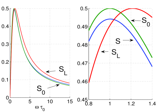
Figure 1: The functions $S$, $S_{L}$, and $S_{0}$ of eq. (84). The right hand frame focuses on the peaks near $\omega\tau_{0}=1$.

The three expressions $S$, $S_{L}$, and $S_{0}$ are compared in Figure 1 as functions of $\omega\tau_{0}$. It is evident from Figure 1 that while the Lagnese and Lions function $S_{L}$ has the same overall behavior as the more precise prediction $S$, the latter is better approximated by $S_{0}$. The maximum absolute error in approximating the sum $S$ by $S_{0}$ is less than $6\times 10^{-3}$. By comparison, the absolute error obtained by approximating $S$ with $S_{L}$ is on the order of 10 times larger. More serious than this, perhaps, is the fact that the frequency at which the maximum of $S_{L}$ occurs is noticeably in error, at $\omega\tau_{0}=12/\pi^{2}=1.216$, see Fig. 1.

It is interesting to note that the maximum of $S$ occurs close to but not exactly at $\omega\tau_{0}=1$. The peak occurs when

$$\frac{S}{\omega\tau_{0}}=\frac{\pi^{2}}{20}=0.4935.$$ (85)

This must be solved numerically for $\omega\tau_{0}$, which can be done using with (84) or the following alternative formula for $S$, which follows from (72), and from [44],

$$S=\frac{6}{x^{3}}\,\bigg{[}x-\bigg{(}\frac{\sin x+\sinh x}{\cos x+\cosh x}\bigg{)}\bigg{]}\,,\qquad x=\frac{\pi}{\sqrt{2}}\,(\omega\tau_{0})^{1/2}\,.$$ (86)

We find that the maximum is at $\omega\tau_{0}=1.0014143\ldots$, and the corresponding maximum value is $S_{\rm max}=0.494178\ldots$. The approximant $S_{0}$ has its maximum precisely at $\omega\tau_{0}=1$, and its maximum value $(1/2)$ is slightly in excess of the correct value $S_{\rm max}$ by about 1%.

4.2. Discussion

We can gain further understanding of the above results by returning to the governing plate equations. The approximation (76) may be interpreted in terms of the in-plane spatial derivatives in both (19b) and (15b). Any variations with wavenumber on the order of $\kappa$ or longer can be safely ignored because the thermal diffusion makes the variation in $z$ dominant. Therefore, for flexural waves and most disturbances associated with thin plate dynamics, we can ignore the $\Delta\Theta$ in (19b) and $\Delta\theta$ in (15b). With the latter approximation, eqs. (15b) and (15c) can be solved to yield eq. (40), as discussed before. In this way the Norris model and the Chadwick model give essentially identical predictions. It also indicates that the Chadwick plate model, while correct, is unnecessarily cumbersome: the in-plane spatial derivatives of temperature can be safely ignored [44]. By the same argument, we may ignore the term $K\Delta\Theta$ in (19b), so that the correspondingly simplified form of the Lagnese and Lions model is

$$C\Theta_{t}+\frac{12}{h^{2}}K\Theta=\frac{\alpha TE}{1-\nu}\,\Delta w_{t}.$$ (87)

This can be solved as

$$\Theta=\frac{\alpha TE}{C(1-\nu)}\,\big{(}\Delta w-g_{L}*\Delta w\big{)}\,,$$ (88)

where

$$g_{L}(t)=\frac{1}{\tau_{L}}\,e^{-t/\tau_{L}}\,.$$ (89)

Substituting from (88) into (19a) it follows that the Lagnese and Lions thermoelastic plate model reduces to

$$(1+\epsilon_{\nu})\,D\Delta^{2}w-\epsilon_{\nu}\,D\,g_{L}*\Delta^{2}w+\rho hw_{tt}=0.$$ (90)

Referring to eqs. (37) and (84), it is clear that the one term damping function $S_{L}$ can be associated with the single relaxation function $g_{L}(t)$ of (89). At the same time, the approximation $S\rightarrow S_{0}$ is equivalent to replacing $g(t)$ of (37) by a simplified relaxation function with a single relaxation time, $g(t)\rightarrow g_{0}(t)$, where

$$g_{0}(t)=\frac{1}{\tau_{0}}\,e^{-t/\tau_{0}}.$$ (91)

Therefore, rather than comparing the frequency domain functions, $S$, $S_{0}$ and $S_{L}$, one can equally well look at the time dependent relaxation functions $g(t)$ of (37), $g_{L}(t)$ of (89), and $g_{0}(t)$ of (91). These are compared in Figure 2.

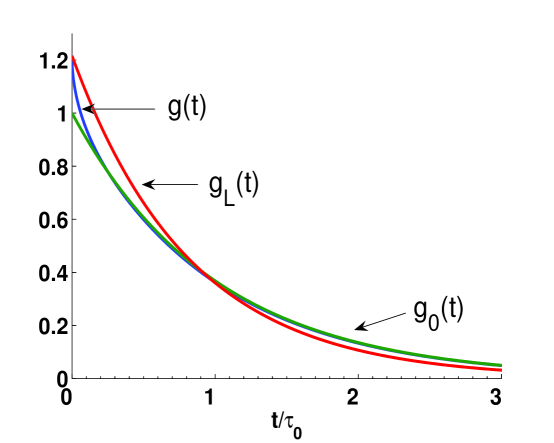
Figure 2: The function $\tau_{0}g(t)$ compared with $\tau_{0}g_{0}(t)$ and $\tau_{0}g_{L}(t)$ .

The relaxation functions $g$, $g_{0}$ and $g_{L}$ share the common property that their integral is unity,

$$\int\limits_{0}^{\infty}g(t)dt=\int\limits_{0}^{\infty}g_{0}(t)dt=\int\limits_{0}^{\infty}g_{L}(t)dt=1,$$ (92)

but the three functions have distinct first moments,

$$\int\limits_{0}^{\infty}\,tg(t)dt=\frac{\pi^{2}}{10}\,\tau_{0},\qquad\int\limits_{0}^{\infty}\,tg_{0}(t)dt=\tau_{0},\qquad\int\limits_{0}^{\infty}\,tg_{L}(t)dt=\frac{\pi^{2}}{12}\,\tau_{0}.$$ (93)

The functions $g(t)$ and $g_{L}(t)$ have the same values at $t=0$, $g(0)=g_{L}(0)=12/(\pi^{2}\tau_{0})$ while $g_{0}(0)=1/\tau_{0}$, as evident from Figure 2. The identities (92) and (93) are associated with the first two terms in the low frequency expansions of the Fourier transforms. The exact transforms are $\widetilde{g}$, defined in (55), and $\widetilde{g}_{0}$ and $\widetilde{g}_{L}$, given by

$$\widetilde{g}_{0}(\omega)=\frac{1}{1-i\omega\tau_{0}},\qquad\widetilde{g}_{L}(\omega)=\frac{1}{1-i\omega\tau_{L}}\,,$$ (94)

and the low frequency expansions are

$$\widetilde{g}(\omega)=1+i\omega\tau_{0}\frac{\pi^{2}}{10}+\ldots\,,\qquad\widetilde{g}_{0}(\omega)=1+i\omega\tau_{0}+\ldots\,,\qquad\widetilde{g}_{L}(\omega)=1+i\omega\tau_{0}\frac{\pi^{2}}{12}+\ldots\,.$$ (95)

Hence, one reason that $g_{0}(t)$ and $S_{0}(\omega)$ are much better approximations than $g_{L}(t)$ and $S_{L}(\omega)$ to the precise quantities $g(t)$ and $S(\omega)$, respectively, is that the number $\pi^{2}/10=0.987$ is closer to unity than $\pi^{2}/12=0.822$.

These results imply that the Lagnese and Lions model could be improved by replacing the term $(h/I)K\Theta=(12/h^{2})K\Theta$ in (16b) with $(10/h^{2})K\Theta$. The resulting simplified single plate equation, analogous to Norris’s equation (36) is then

$$(1+\epsilon_{\nu})\,D\Delta^{2}w-\epsilon_{\nu}\,D\,g_{0}*\Delta^{2}w+\rho hw_{tt}=0.$$ (96)

Note the relaxation function is now $g_{0}$, rather than $g_{L}$ as in eq. (90). The use of $g_{L}$ produces the inaccuracies shown in Figures 1 and 2, while the same Figures illustrate that $g_{0}$ is a far better approximation to $g(t)$.

The derivation of eq. (96) as an improvement on (90) indicates that the source of the discrepancy in the Lagnese and Lions model can be partly ascribed to the term $(h/I)K\Theta$ in eq. (19b). As noted before, the term in question originates in the evaluation of $(K/I)\mu$ where the first moment of $-\theta_{zz}$ is defined in (17) and evaluated, according to the linear approximation for $\theta$ assumed by Lagnese and Lions, in (18). Equation (18) is incorrect. The correct form follows from Norris and Photiadis [44], and is most readily expressed in the frequency domain, as

$$\widetilde{\theta}(x,y,z,\omega)=\frac{1}{1-\widetilde{g}(\omega)}\,\big{(}z-\frac{\sin\gamma z}{\gamma\cos\gamma\frac{h}{2}}\big{)}\,\widetilde{\Theta}(x,y,\omega),$$ (97)

where $\gamma$ and $\widetilde{g}(\omega)$ are defined in eqs. (44) and (55), respectively. Thus, eqs. (17) and (97) imply

$$\widetilde{\mu}=\big{[}\frac{1-\big{(}\gamma\frac{h}{2}\big{)}^{-1}\tan\gamma\frac{h}{2}}{1-\widetilde{g}(\omega)}\big{]}\,h\widetilde{\Theta},$$ (98)

and expanding,

$$\widetilde{\mu}=\big{[}\frac{5}{6}-\frac{(\gamma h)^{2}}{1008}+\mbox{O}\big{(}\gamma^{4}h^{4}\big{)}\big{]}\,h\widetilde{\Theta}.$$ (99)

This suggests that a better approximation than that of Lagnese and Lions is to take the leading order term,

$$\mu=\frac{5}{6}\,h\Theta,$$ (100)

which in turn implies the modified governing equation (96).

What are the relative benefits of the four different models? The results presented indicate that for the infinite plate, one might just as well use the Norris model, since it is almost the simplest (only Simmond’s is simpler) yet it provides the same accuracy as that of Chadwick. The equivalence rests on the fact that for any practical plate of thickness $h$, one must have $h\gg l$, the mean free path of the thermal phonons. It might be argued that the other models are more appropriate for finite systems, i.e. plates with edges subject to a variety of boundary conditions. We have not discussed the edge conditions for each model, as this is a large topic in itself [2, 4]. Suffice to say that for each model one can define appropriate conditions that supplement the governing equations and define a closed problem for a given practical situation.

In order to examine the utility of the models for a finite plate, Appendix D discusses the solution for the case of a beam with fixed ends and zero heat flux at the ends within the context of the Lagnese and Lions model. The results there indicate that the additional equation (19b) for $\Theta$ only effects the solution in a boundary layer at the edges. The Norris and Simmonds models do not provide a boundary layer solution, but have solutions analogous to the classical Kirchhoff theory but with modified (complex valued) flexural wavenumber. Once could argue that the Lagnese and Lions model is useful in that it provides a boundary layer, even though the layer, being exponentially narrow, has insignificant effect on the value of both the modal frequencies and damping of the oscillating modes (see [4] for further details). The presence of a boundary layer at the edges is expected, and while the Lagnese and Lions model predicts one, only the Chadwick model is capable of providing the proper description of the boundary layer. Thus, the width of the boundary layer of the Lagnese and Lions model is O$(\delta^{1/2}/\kappa)$ where $\delta$ is defined in eq. (73) and $\kappa$ is the classical flexural wavenumber. This boundary layer width could be less than, on the order of, or larger than the plate thickness, depending on the material parameters. One can envisage circumstances in which the boundary layer width is less than $h$, and consequently will have $z-$ dependence. This is not contained within the Lagnese and Lions model and can only be captured by the Chadwick model. This fundamental difficulty arises with all beam and shell theories, classical or higher-order: they do not accurately describe edge boundary layers that vary over a distance O$(h)$. However, regardless of the precise nature of the temperature field near the boundary, it will have essentially no effect upon the modal properties of the plate (frequency, damping, mode shape, etc.).

5 Conclusion

We have compared four distinct models for flexural motion of thermoelastic thin plates, with specific attention to the leading order effects on wave damping. Of the four, the Chadwick theory is expected to be the most reliable as it retains the 3D nature of the thermal field. While the Lagnese and Lions has the same overall behavior as Chadwick’s in terms of frequency, there is a distinct quantitative difference. This is attributable to the approximation of the first moment of the temperature, which is inaccurately accounted for by the Lagnese and Lions model. The relatively simple single equation of Simmonds predicts the correct low frequency behavior but is incorrect for medium and high frequencies. The reason is that the Simmonds equations approximates the thermoelastic effect as a simple viscous damping term which does not capture the full frequency content. Comparisons of the Norris model with that of Chadwick indicates that the former adequately predicts the full frequency behavior. The single equation of Norris provides an accurate approximation because the the dominant variation in the temperature field is in the through thickness direction, which permits it to be replaced by an equivalent viscoelastic term. The Norris model retains the simplicity of a single uncoupled equation for plate deflection, but provides a more accurate representation of the thermoelastic “hidden variables” than Simmonds’. The Lagnese and Lions model misses the crucial point that the dependence of $\theta$ on the in-plane coordinates $x$ and $y$ is secondary to its dependence upon $z$. This permits considerable simplification with the result that a separate equation for temperature is not necessary. Instead, the temperature is incorporated into the classical plate equation as an effective viscoelastic relaxation [4]. Of the four models, the simpler single equation of Norris captures the thermal mechanics of the more general Chadwick theory, and is to be preferred to the other models considered.

Appendix A: A correction to the Lagnese and Lions equations

In this Appendix the correction to eqs. (16a) is obtained by the same method used in the original derivation of Lagnese and Lions [2]. The cause of the Lagnese and Lions error is that the energy density $U$ (different notation) is defined in [2] by $U=\frac{1}{2}\mbox{\boldmath${\sigma}$}\cdot\mbox{\boldmath${\varepsilon}$}$. The correct energy density for the conjugate independent variables strain and temperature is the Helmholtz free energy $F$, see e.g. [44], where $F=\frac{1}{2}(\mbox{\boldmath${\sigma}$}\cdot\mbox{\boldmath${\varepsilon}$}-s\theta)$. Using equations (13) and (1), the total strain energy becomes

$${\cal F}=\frac{1}{2}\int\limits_{\Omega}\bigg{\{}D\big{[}(\Delta w)^{2}-2(1-\nu)\big{(}w_{11}w_{22}-w_{12}^{2}\big{)}+2(1+\nu)\alpha\theta\Delta w\big{]}-\frac{C}{T}\theta^{2}\bigg{\}}dxdy\,.$$ (A.1)

The analogous equation (6.7) in [2] omits the final term and the coefficient of the $(1+\nu)\alpha\theta\Delta w$ term is unity rather than $2$, and hence the error in (16a).

Appendix B:

The functions defined by (26) may be found recursively as follows,

$$u^{(n)}(s)=\sum\limits_{j=0}^{n}\,a^{n}_{j}\,\frac{s^{2n-2j+1}}{2n-2j+1},$$ (B.1)

with

$$a^{n}_{j}=\frac{a^{n-1}_{j}}{(2n-2j)(2n-2j-1)},\,\,n>j\geq 0;\qquad a^{n}_{n}=-\sum\limits_{j=0}^{n-1}\,a^{n}_{j},\,\,n>0;\qquad a^{0}_{0}=1.$$ (B.2)

The values $u^{(n)}(1)$ in eq. (30) can be found using these recursion relations. We now demonstrate another, more constructive, way to obtain these coefficients. The series expansion (30) may be obtained from the Norris solution for $\Theta$ written in the frequency domain as

$$\widetilde{\Theta}(x,y,\omega)=\frac{\alpha TE}{C(1-\nu)}\,\big{[}1-\widetilde{g}(\omega)\big{]}\,\Delta\widetilde{w},$$ (B.3)

where $\widetilde{g}(\omega)$ is given in (55). The latter may be expanded in a Taylor series as

$$\widetilde{g}(\omega)=\sum\limits_{m=0}^{\infty}\,S_{m}\,(i\omega)^{m},\qquad\mbox{where}\quad S_{m}=\sum\limits_{n=0}^{\infty}\,d_{n}\tau_{n}^{m}\,.$$ (B.4)

The infinite series $S_{m}$ may be evaluated using (38), and known results [48], as

$$S_{m}=\tau_{0}^{m}\,48\,\pi^{2m}\big{(}2^{2m+4}-1\big{)}\,\frac{|B_{2m+4}|}{(2m+4)!}\,,$$ (B.5)

where $B_{m}$ are the Bernoulli numbers [49]. Eliminating $\tau_{0}$ in favor of $\tau_{S}$ of (29) gives

$$S_{m}=3\,\tau_{S}^{m}\,2^{2m+4}\big{(}2^{2m+4}-1\big{)}\,\frac{|B_{2m+4}|}{(2m+4)!}\,,$$ (B.6)

and hence

$$\widetilde{g}(\omega)=1+\frac{2}{5}\,i\omega\tau_{S}+\frac{17}{105}\,(i\omega\tau_{S})^{2}+\frac{62}{945}\,(i\omega\tau_{S})^{3}+\ldots.$$ (B.7)

Equation (30) then follows from (B.3), (B.7) and the connection $-i\omega\rightarrow\partial/\partial t$. Finally, convergence properties of the series $(\ref{bb2})_{1}$ follow from the behavior of the Bernoulli numbers for large index. Omitting the details, it may be shown that the series is unconditionally convergent for $\omega\tau_{0}<e$.

Appendix C: Alternative justification of the $F_{0}$ approximation

The justification for the approximation of $F_{0}$ (eqs. (65) and (72)) is discussed further. If the reader is uncomfortable with the argument based on the requirement that the phonon mean free path must be much shorter than the plate thickness, an alternative reason is given here. We focus directly on the damping defined in (56) as given by eq. (57). Thus,

$$Q^{-1}=-\epsilon_{\nu}\pi^{2}\,\omega\tau_{0}\,\mbox{Re}\,F_{0}\,,$$ (C.1)

where $F_{0}$ is given by (65).

The Lagnese and Lions model is considered first. It follows from (C.1) that

$$Q^{-1}=\epsilon_{\nu}\frac{\omega\tau_{*}}{1+\omega^{2}\tau_{*}^{2}},\quad\mbox{Lagnese and Lions},$$ (C.2)

where

$$\tau_{*}=\frac{\pi^{2}\,\tau_{0}}{12+(\kappa h)^{2}}.$$ (C.3)

The thin plate model, whether thermoelastic or classical, is premised on the long wavelength assumption that

$$\kappa h\ll 1.$$ (C.4)

Therefore,

$$\tau_{*}=\frac{\pi^{2}}{12}\,\tau_{0}+\mbox{O}[(\kappa h)^{2}]\,,$$ (C.5)

and it is entirely consistent with the thin plate theory (Kirchhoff approximation) to take $\tau_{*}=\tau_{0}\pi^{2}/12$, i.e., $\tau_{*}=\tau_{L}$.

For the Chadwick model, eqs. (56), (57) and (55) imply

$$Q^{-1}=\epsilon_{\nu}\sum\limits_{n=0}^{\infty}\,\frac{d_{n}\omega\tau_{n*}}{1+\omega^{2}\tau_{n*}^{2}},\quad\mbox{Chadwick},$$ (C.6)

with

$$\tau_{n*}=\frac{\tau_{n}}{1+(\frac{\kappa h}{\pi})^{2}\frac{\tau_{n}}{\tau_{0}}}.$$ (C.7)

Invoking the necessary condition (C.4), we have

$$\tau_{n*}=\tau_{n}+\mbox{O}(\kappa^{2}h^{2})\,,$$ (C.8)

and consequently, to the same order of accuracy, i.e. ignoring O$(\kappa^{2}h^{2})$,

$$Q^{-1}=\epsilon_{\nu}\sum\limits_{n=0}^{\infty}\,\frac{d_{n}\omega\tau_{n}}{1+\omega^{2}\tau_{n}^{2}},\quad\mbox{Chadwick}.$$ (C.9)

Appendix D: Solutions for a finite plate or beam

We consider a plate of finite extent in the $x-$direction, $-L\leq x\leq L,\,-\infty<y<\infty$, with motion independent of $y$. The ends are assumed, for simplicity, as fixed, with zero heat flux. The problem is completely analogous to that of a beam, which is simply the limit of a plate of vanishing width in the $y-$direction [50]. The beam solution is obtained by setting $\nu\rightarrow 0$ but for consistency we will stay with the plate problem here.

For simplicity, we only seek solutions that are symmetric in $x$, i.e. of the form

$$w(x,t)=\sum\limits_{i=1}^{3}A_{i}\,\cos(k_{i}x-\omega t),\qquad\Theta(x,t)=\sum\limits_{i=1}^{3}\rho_{i}A_{i}\,\cos(k_{i}x-\omega t),$$ (D.1)

where $\pm k_{i}$, $i=1,2,3$ are the three independent roots of (45) and $\rho_{i}$ follow from (19a) as

$$\rho_{i}=\frac{k_{i}^{4}-\kappa^{4}}{k_{i}^{2}\alpha(1+\nu)}=\frac{\epsilon_{\nu}\gamma^{2}k_{i}^{2}}{\alpha(1+\nu)(k_{i}^{2}-\gamma^{2}+\frac{12}{h^{2}})}\,.$$ (D.2)

The end conditions

$$w(\pm L,t)=w_{x}(\pm L,t)=\theta_{x}(\pm L,t)=0\,,$$ (D.3)

imply

$$\left[\begin{array}[]{ccc}\cos k_{1}L&\cos k_{2}L&\cos k_{3}L\\ &&\\ k_{1}\sin k_{1}L&k_{2}\sin k_{2}L&k_{3}\sin k_{3}L\\ &&\\ \rho_{1}k_{1}\sin k_{1}L&\rho_{2}k_{2}\sin k_{2}L&\rho_{3}k_{3}\sin k_{3}L\end{array}\right]\left[\begin{array}[]{c}A_{1}\\ \\ A_{2}\\ \\ A_{3}\end{array}\right]=0\,,$$ (D.14)

and in order that we have a non-trivial solution, $(\omega,\,k)$ must satisfy the dispersion relation

$$\left|\begin{array}[]{ccc}\cos k_{1}L&\cos k_{2}L&\cos k_{3}L\\ &&\\ k_{1}\sin k_{1}L&k_{2}\sin k_{2}L&k_{3}\sin k_{3}L\\ &&\\ \rho_{1}k_{1}\sin k_{1}L&\rho_{2}k_{2}\sin k_{2}L&\rho_{3}k_{3}\sin k_{3}L\end{array}\right|=0\,.$$ (D.20)

Let $k_{1}$ and $k_{2}$ correspond to the roots which are close to (within order $\epsilon_{\nu}$) the elastic roots $\pm\kappa$ and $\pm i\kappa$ (i.e. the roots of $k^{4}-\kappa^{4}=0$). The wavenumber $k_{3}$ is, to leading order, given by

$$k_{3}^{2}\approx\gamma^{2}-\frac{12}{h^{2}}\,.$$ (D.21)

It follows that

$$\left|\frac{\rho_{1}}{\rho_{3}}\right|,\,\left|\frac{\rho_{2}}{\rho_{3}}\right|\approx\left|\frac{\epsilon_{\nu}\kappa^{2}\gamma^{2}}{k_{3}^{2}(\gamma^{2}-\frac{12}{h^{2}})}\right|=\mbox{O}\big{(}\epsilon_{\nu}\delta\big{)},$$ (D.22)

where $\delta\ll 1$ is defined in (73). Thus,

$$|\rho_{1}|,\,|\rho_{2}|\ll|\rho_{3}|,$$ (D.23)

which enables approximation of eq. (D.20) as

$$\left|\begin{array}[]{cc}\cos k_{1}L&\cos k_{2}L\\ &\\ k_{1}\sin k_{1}L&k_{2}\sin k_{2}L\end{array}\right|=0\,.$$ (D.27)

To be more precise, $k_{1},\,k_{2}$ are roots of $k^{4}-{\kappa^{\prime}}^{4}=0$ where the complex valued wavenumber $\kappa^{\prime}$ follows from (66),

$${\kappa^{\prime}}^{4}=\kappa^{4}\big{[}1-\epsilon_{\nu}\,f(\gamma h)\big{]},$$ (D.28)

and $f$ is defined in (72). Thus, to leading order in the thermoelasticity the dispersion relation is, from (D.27),

$$\tan\kappa^{\prime}L+\tanh\kappa^{\prime}L=0\,.$$ (D.29)

It is important to note that this dispersion relation has the same form as that of the elastic plate or beam without thermoelasticity. The latter is obtained by the reduction $\kappa^{\prime}\rightarrow\kappa$. Thermoelasticity has the effect of modifying the wavenumber in the same way that it is altered in the infinite system, and the end conditions do not introduce any new effects. In fact, it can be easily checked that the dispersion relation (D.29) is also obtained if one uses the Norris equation, which does not include temperature explicitly (and therefore does not require an end condition associated with temperature).

The above result can be explained in terms of boundary layers at the two ends. In order to see this from the full solution for the Lagnese & Lions model, we note that $\rho_{1}$ and $\rho_{2}$ may be approximated using (75), and combined with (D.14) the leading order solution can be shown to be

$$w \approx A_{0}\bigg{(}\sinh\kappa L\cos\kappa x+\sin\kappa L\cosh\kappa x+\frac{\epsilon_{\nu}2\kappa^{3}\gamma^{2}}{k_{3}^{3}(\gamma^{2}-\frac{12}{h^{2}})}\sin\kappa L\sinh\kappa L\frac{\cos k_{3}x}{\sin k_{3}L}\bigg{)},$$

$$\Theta \approx \frac{\epsilon_{\nu}2\kappa^{2}\gamma^{2}A_{0}}{\alpha(1+\nu)(\gamma^{2}-\frac{12}{h^{2}})}\bigg{(}-\sinh\kappa L\cos\kappa x+\sin\kappa L\cosh\kappa x+\frac{2\kappa}{k_{3}}\sin\kappa L\sinh\kappa L\frac{\cos k_{3}x}{\sin k_{3}L}\bigg{)}.$$

With no loss in generality, choose $k_{3}$ as the root with positive imaginary part. Then $|e^{ik_{3}L}|\ll|e^{-ik_{3}L}|$, and consequently, for positions not near the center of the plate, we have

$$\Theta\approx\frac{\epsilon_{\nu}2\kappa^{2}\gamma^{2}A_{0}}{\alpha(1+\nu)(\gamma^{2}-\frac{12}{h^{2}})}\bigg{(}-\sinh\kappa L\cos\kappa x+\sin\kappa L\cosh\kappa x-i\frac{\kappa}{k_{3}}\sin\kappa L\sinh\kappa L\,e^{ik_{3}(L-|x|)}\bigg{)},$$ (D.31)

with a similar equation for $w$. While (D.31) is not valid at the center $(x=0)$ it provides a faithful leading order approximation near the ends. The decay is far more rapid than that of the evanescent flexural wave, since Im$(k_{3}/\kappa)\gg 1$ (see eqs. (73) and (75)). This indicates that the contribution of the complex wavenumber $k_{3}$ is an exponentially decaying boundary layer. The fact that $|k_{3}|h$ is on the order of or larger than unity raises doubts about the utility of the model, particularly near boundaries.

Acknowledgment: Comments from Prof. James G. Simmonds are appreciated.

References

- [1] P. Chadwick. On the propagation of thermoelastic disturbances in thin plates and rods. J. Mech. Phys. Solids, 10:99–109, 1962.
- [2] J. E. Lagnese and J.-L. Lions. Modelling Analysis and Control of Thin Plates. Paris, Masson, 1988.
- [3] J. G. Simmonds. Major simplifications in a current linear model for the motion of a thermoelastic plate. Q. Appl. Math., 57(4):673–679, 1999.
- [4] A. N. Norris. Flexural vibration and thermoelastic damping of thin plates: A simplified model. to be submitted, 2005.
- [5] D. M. Photiadis, B. H. Houston, X. Liu, J. A. Bucaro, and M. H. Marcus. Thermoelastic loss observed in a high Q mechanical oscillator. Physica B., 316:408–410, 2002.
- [6] Y. T. Liu and K. S. Thorne. Thermoelastic noise and homogeneous thermal noise in finite sized gravitational-wave test masses. Phys. Rev. D, 62:122002, 2000.
- [7] C. Zener. General theory of thermoelastic internal friction. Phys. Rev., 53:90–99, 1938.
- [8] J. B. Alblas. On the general theory of thermo-elastic friction. Appl. Sci. Res., A10:349–362, 1961.
- [9] J. B. Alblas. A note on the theory of thermoelastic damping. J. Thermal Stresses, 4:333–355, 1981.
- [10] R. Lifshitz and M. L. Roukes. Thermoelastic damping in micro- and nanomechanical systems. Phys. Rev. B, 61(8):5600–5609, 2000.
- [11] J. E. Lagnese. Boundary Stabilization of Thin Plates, volume 10 of SIAM Studies in Applied Mathematics. SIAM, Philadelphia, 1989.
- [12] J. Lagnese. The reachability problem for thermoelastic plates. Arch. Rat. Mech. Anal., 112:223–267, 1990.
- [13] G. Avalos and I. Lasiecka. Exponential stability of a thermoelastic system with free boundary conditions without mechanical dissipation. SIAM J. Math. Anal., 29:155–182, 1998.
- [14] G. Avalos and I. Lasiecka. Exact-approximate boundary reachability of thermoelastic plates under variable thermal coupling. Inverse Problems, 16:979–996, 2000.
- [15] G. Avalos and I. Lasiecka. Boundary controllability of thermoelastic plates with free boundary conditions. SIAM J. Control Optim., 38:337–383, 2000.
- [16] G. Avalos and I. Lasiecka. The null controllability of thermoelastic plates and singularity of the associated minimal energy function. J. Math. Anal. Appl., 294:34–61, 2004.
- [17] J. E. M. Rivera and Y. Shibata. A linear thermoelastic plate equation with Dirichlet boundary condition. Math. Meth. Appl. Sc., 20:915–932, 1997.
- [18] J. E. M. Rivera and R. K. Barreto. Decay rates of solutions to thermoviscoelastic plates with memory. IMA J. Appl. Math., 60:263–283, 1998.
- [19] J. E. M. Rivera and L. H. Fatori. Regularizing properties and propagations of singularities for thermoelastic plates. Math. Meth. Appl. Sc., 21:797–821, 1998.
- [20] J. E. M. Rivera and H. P. Oquendo. The transmission problem for thermoelastic beams. J. Thermal Stresses, 24:1137–1158, 2001.
- [21] M. Eller, I. Lasiecka, and R. Triggiani. Simultaneous exact/approximate boundary controllability of thermo-elastic plates with variable thermal coefficient and moment control. J. Math. Anal. Appl., 251:452–478, 2000.
- [22] M. Eller, I. Lasiecka, and R. Triggiani. Exact/approximate controllability of thermoelastic plates with variable thermal coefficients. Discrete Control. Dyn. Sys., 7:283–302, 2001.
- [23] I. Lasiecka, M. Renardy, and R. Triggiani. Backward uniqueness for thermoelastic plates with rotational forces. Semigroup Forum, 62:217–242, 2001.
- [24] V. Isakov. On the uniqueness of the continuation for a thermoelasticity system. SIAM J. Math. Anal., 33:509–522, 2001.
- [25] S. W. Hansen and B. Y. Zhang. Boundary control of a linear thermoelastic beam. J. Math. Anal. Appl., 201:182–205, 1997.
- [26] A. K. Nandakumaran and R. K. George. Exact controllability of a semilinear thermoelastic system. Num. Fun. Anal. Opt., 25:271–285, 2004.
- [27] K. T. Andrews, J. R. Fernandez, and M. Shillor. A thermoviscoelastic beam with a tip body. Comp. Mech., 33:225–234, 2004.
- [28] M. Grobbelaar-Van Dalsen. Uniform stabilization of a one-dimensional hybrid thermo-elastic structure. Math. Meth. Appl. Sc., 26:1223–1240, 2003.
- [29] G. Lebeau and E. Zuazua. Null-controllability of a system of linear thermoelasticity. Arch. Rat. Mech. Anal., 141:457–482, 1998.
- [30] C. Giorgi, V. Pata, and N. Bellomo. Stability of abstract linear thermoelastic systems with memory. Math. Models Meth. Appl. Sc., 11:627–644, 2001.
- [31] Y. Enomoto. On a thermoelastic plate equation in an exterior domain. Math. Meth. Appl. Sc., 25:443–472, 2002.
- [32] H. Leiva and Z. Sivoli. Existence, stability and smoothness of a bounded solution for nonlinear time-varying thermoelastic plate equations. J. Math. Anal. Appl., 285:191–211, 2003.
- [33] Z.-Y. Liu and M. Renardy. A note on the equations of a thermoelastic plate. Appl. Math. Lett., 9:1–6, 1995.
- [34] Z. Liu and S. Zheng. Exponential stability of the Kirchhoff plate with thermal or viscoelastic dampings. Q. Appl. Math., 15:551–564, 1997.
- [35] J. U. Kim. On the energy decay of a linear thermoelastic bar and plate. SIAM J. Math. Anal., 23:889 899, 1992.
- [36] Y. Shibata. On the exponential decay of the energy of a linear thermoelastic plate. Comp. Appl. Math., 13:81 102, 1994.
- [37] L. de Teresa and E. Zuazua. Controllability of the linear system of thermoelastic plates. Adv. Differential Equations, 1:369–402, 1996.
- [38] A. Benabdallah and D. Teniou. Exponential stability of a Von Karman model. Electronic J. Diff. Equat., 1998:1–13, 1998.
- [39] A. Benabdallah and M. G. Naso. Null controllability of a thermoelastic plate. Abstract Appl. Analysis, 7:585–599, 2002.
- [40] G. Amendola. Existence, uniqueness, and asymptotic sstability for a thermoelastic plate. Nonlinear Oscillations, 6:145–163, 2003.
- [41] D. B. Henry, A. Perissinitto, and O. Lopes. On the essential spectrum of a semigroup of thermoelasticity. Nonlinear Anal. Theory Methods Appl., 21:65–75, 1993.
- [42] K. S. Liu and Z. Y. Liu. Exponential stability and analyticity of abstract linear thermoelastic systems. Z. Angew. Math. Phys., 48:885–904, 1997.
- [43] C. Giorgi and M. G. Naso. Mathematical models of thin thermoviscoelastic plates. Q. J. Mech. Appl. Math., 53:363–374, 2000.
- [44] A. N. Norris and D. M. Photiadis. Thermoelastic relaxation in elastic structures, with applications to thin plates. Q. J. Mech. Appl. Math., 2005.
- [45] S. Timoshenko and S. Woinowsky-Krieger. Theory of Plates and Shells. McGraw-Hill, New York, 1987.
- [46] W. Nowacki. Dynamic Problems in Thermoelasticity. Noordhoff, Leyden, 1989.
- [47] C. Kittel. Elementary Statistical Physics. John Wiley & Sons, Inc. New York, 1958.
- [48] Wolfram Research, Inc. Mathematica. Version 5.0 edition, 2003.
- [49] I. S. Gradshteyn, I. M. Ryzhik, Alan Jeffrey, and Daniel Zwillinger. Table of Integrals, Series, and Products. Academic Press, 2000.
- [50] A. N. Norris. Flexural waves on narrow plates. J. Acoust. Soc. Am., 113:2647–2658, 2003.