Exact Shock Profile for the ASEP with Sublattice-Parallel Update

Abstract

We analytically study the one-dimensional Asymmetric Simple Exclusion Process (ASEP) with open boundaries under sublattice-parallel updating scheme. We investigate the stationary state properties of this model conditioned on finding a given particle number in the system. Recent numerical investigations have shown that the model possesses three different phases in this case. Using a matrix product method we calculate both exact canonical partition function and also density profiles of the particles in each phase. Application of the Yang-Lee theory reveals that the model undergoes two second-order phase transitions at critical points. These results confirm the correctness of our previous numerical studies.
Key words: Shock, Reaction-Diffusion, Matrix Product Formalism
PACS: 05.20.-y, 02.50.Ey, 05.70.Fh, 05.70.Ln

1 Introduction

The study of steady states of non-equilibrium systems has motivated a lot of works over the last decades [1, 2, 3]. These models exhibit in general shock structures in their steady state. The study of microscopic and macroscopic structure of shocks in one-dimensional reaction-diffusion models has also been one of physicists’ interests recently [4, 5, 6, 7]. The most well known model which reveals shocks in the steady state is Asymmetric Simple Exclusion Process (ASEP) with open boundaries [8, 9]. The ASEP is a model of diffusing identical classical particles with hardcore interactions on a one-dimensional lattice. In this model particles are injected from left boundary of a lattice of length $L$ with rate $\alpha$ provided that the first site is empty. They hop to right in the bulk of that lattice with finite rate and leave it from right boundary with rate $\beta$ provided that the last site is already occupied. A substantial amount of exact results have been obtained for the ASEP which include the phase diagram, stationary state probability distribution function, correlation functions and correlation lengths. It is also known that for special tuning of microscopic rates a travelling shock with a step-like density profile evolves in the system. The phase diagram of the ASEP with random sequential updating scheme (continuous-time) has three different phases: a low-density phase, a high-density phase and a maximal-current phase. The shocks appear on the coexistence line between the low-density and high-density phases, however; for the ASEP with open boundaries the shock can be anywhere on the lattice with equal probabilities and the resulting profile in the steady state is linear. In order to study the dynamics of the shocks in the ASEP, the model been considered on a lattice with periodic boundary condition in the presence of a second-class particle (often called an impurity) [2, 5, 10]. In this case the density profile of the particles, as seen from the impurity, is a step-like function i.e. a discontinuity between a low-density and a high-density region with an interface which is sharp on lattice scale.
Despite the remarkable work on the microscopic structure of shocks and their dynamics in continuous-time update [4, 5, 6], not much has been known about that in discrete-time updates. For the ASEP in sublattice-parallel update the temporal evolution of a single shock has been studied [7]. By making use of a quantum algebra symmetry of the generator of the process it has been shown that on the microscopic level the dynamics of the shock can be described by a single particle dynamics in the thermodynamic limit. In the present paper we study the microscopic structure of the shocks in the ASEP in sublattice-parallel dynamics; however, instead of introducing a second-class particle, we consider the case where the total number of particles is kept fixed.
The ASEP under sublattice-parallel update with open boundaries was first introduced and studied in [11]. In this model particles are injected from the left boundary with probability $\alpha$ and extracted from the right boundary with probability $\beta$. In the bulk of the lattice they hop to the right with unit probability. The exact phase diagram and stationary density profile of the particles in this case (without conditioning on the particle number) have been obtained in the same reference. Later this model was studied using a matrix product method and the same results were obtained [12]. However, the case of fixed particle number has not been studied yet.
Our recent numerical investigations show that in the case of fixed particle number the phase diagram of the model highly depends on the total density of the particles on the lattice $\rho$, $\alpha$ and $\beta$ [13]. For $\rho<\frac{1}{2}$ the phase diagram contains a low-density and a shock phase while for $\rho>\frac{1}{2}$ it has a high-density phase and also a shock phase. In both cases the phase transition points $(\alpha_{c},\beta_{c})$ are determined by the total density of particles $\rho$. The density profile of the particles in the steady state have also been studied for both even and odd sites. In low-density (high-density) phase $\rho<\frac{1}{2},\beta>\beta_{c}$ ($\rho>\frac{1}{2},\alpha>\alpha_{c}$) the density profile of the particles for both even and odd sites is a constant on the lattice except near the left (right) boundary where it becomes an exponentially increasing (decreasing) function of site number. In the shock phase $\rho<\frac{1}{2},\beta<\beta_{c}$ or $\rho>\frac{1}{2},\alpha<\alpha_{c}$ the density profile of the particles for both even and odd sites is an error function.
In this paper we continue our studies analytically. Using a matrix product formalism, in which the steady state weights are written in terms of the expectation value of product of non-commuting operators, we calculate the canonical partition function of the model exactly. The thermodynamic behavior of this function will also be calculated in each of three phases mentioned above. The exact expressions for the density profile of the particles in each phase have also been calculated. Recently it has been shown that the classical Yang-Lee theory of equilibrium phase transitions [14] can be applied to the non-equilibrium models to study their out of equilibrium phase transitions (for a review see [15]). The simplicity of our model allows us to calculate the line of the canonical partition function zeros in the thermodynamic limit from which we obtain the critical points. In analogy with equilibrium statistical mechanics one can introduce the pressure (which is obviously not the physical pressure of the particles) and study its behavior as a functions of $\rho^{-1}$ for fixed $\alpha$ and $\beta$. It turns out that resulting curve looks quite similar to the isotherm of a Bose gas when Bose-Einstein condensation takes place.
Our paper is organized as follows: In section 2 we will define the model and calculate its steady state probability distribution function using a matrix product formalism. The canonical partition function of the model will also be calculated. In section 3 the density profile of the particles on the lattice will be obtained. In section 4 we will apply the Yang-Lee theory to study the phase transitions in the model and also study its similarities with a Bose gas. Finally in section 5 we will discuss the results.

2 Canonical partition function

The ASEP with sublattice-parallel update is defined as follows: Classical particles hop deterministically on a one-dimensional lattice of length $L$ which is assumed to be an even number. The system is updated in two half time steps. In the first half time step the leftmost and the rightmost sites and also the particles at even sites are updated. They are injected to the leftmost site with probability $\alpha$ provided that the first site is empty. The particles at even sites will hop to their rightmost neighbors provided that the target sites are empty. If the last site of the lattice is occupied it will be extracted with probability $\beta$. In the second half-time step only the particles at odd sites will be updated according to the bulk dynamics mentioned above. These two steps are shown in Fig. 1.

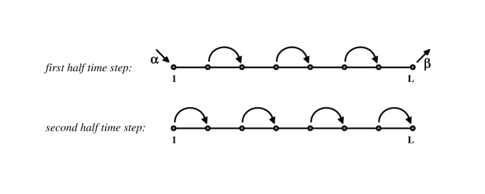
Figure 1: The ASEP under sublattice-parallel updating scheme.

From now on we assume that the total density of particles on the lattice is kept fixed $\rho=\frac{M}{L}$ in which $M$ is the total number of particles. In order to study the steady state properties of this model analytically we will adopt a so called Matrix Product Formalism (MPF). In what follows we will briefly review the MPF for the ASEP with sublattice-parallel dynamics first introduced in [12]. Let us define the occupation number at site $i$ as $\tau_{i}\in\{0,1\}$ where $\tau_{i}=1$ if it is occupied and $\tau_{i}=0$ if it is empty. Now according to the MPF, the stationary state probability for the system to be in a given configuration $\{\tau\}=\{\tau_{1},\cdots,\tau_{L}\}$ with exactly $M$ particles is given by

$$P(\{\tau\})\propto\delta(M-\sum_{i=1}^{L}\tau_{i})\langle W|\prod_{i=1}^{\frac{L}{2}}[\hat{\mathcal{O}}_{2i-1}\mathcal{O}_{2i}]|V\rangle$$ (1)

where we have defined

$$\hat{\mathcal{O}}_{i}:=\tau_{i}\hat{D}+(1-\tau_{i})\hat{E}\;,\;\mathcal{O}_{i}:=\tau_{i}D+(1-\tau_{i})E.$$ (2)

The Dirac $\delta$ in (1) guarantees the conservation of the total number of particles. For the ASEP with sublattice-parallel dynamics the operators ($\hat{D},\hat{E}$) and ($D,E$) are finite dimensional square matrices and with the vectors $|V\rangle$ and $\langle W|$ satisfy the following quadratic algebra

$$\begin{array}[]{l}[E,\hat{E}]=[D,\hat{D}]=0\;,\;E\hat{D}=[\hat{E},D]\;,\;\hat{D}E=0\\ \langle W|\hat{E}(1-\alpha)=\langle W|E\;,\;\langle W|(\alpha\hat{E}+\hat{D})=\langle W|D\\ (1-\beta)D|V\rangle=\hat{D}|V\rangle\;,\;(E+\beta D)|V\rangle=\hat{E}|V\rangle.\end{array}$$ (3)

The operators ($\hat{D},\hat{E}$) and ($D,E$) stand for the presence of particles and holes at odd and even sites respectively. It has also been shown that (3) has a two-dimensional representation for $\alpha\neq\beta$ given by [12]

$$\begin{array}[]{l}\hat{D}=\left(\begin{array}[]{cccc}\alpha(1-\beta)&&&0\\ -\alpha\beta&&&0\end{array}\right)\;,\;\hat{E}=\left(\begin{array}[]{cccc}\alpha\beta&&&0\\ \alpha\beta&&&\beta\end{array}\right)\;,\;|V\rangle=\left(\begin{array}[]{c}1-\beta\\ -\beta\end{array}\right)\\ \\ D=\left(\begin{array}[]{cccc}\alpha&&&0\\ -\alpha\beta&&&\alpha\beta\end{array}\right)\;,\;E=\left(\begin{array}[]{cccc}0&&&0\\ \alpha\beta&&&\beta(1-\alpha)\end{array}\right)\;,\;\langle W|=(\alpha,1-\alpha).\end{array}$$ (4)

The normalization factor in (1), which will be called the canonical partition function of the model, should be obtained using the fact that the steady state probability distribution function $P(\{\tau\})$ is normalized i.e. $\sum_{\{\tau\}}P(\{\tau\})=1$. It can now be written as

$$Z_{L,M}=\sum_{\{\tau\}}\delta(M-\sum_{i=1}^{L}\tau_{i})\langle W|\prod_{i=1}^{\frac{L}{2}}[\hat{\mathcal{O}}_{2i-1}\mathcal{O}_{2i}]|V\rangle.$$ (5)

The canonical partition function of the model $Z_{L,M}$ is a key function in calculating the physical quantities such as the density profile of the particles on the lattice in the steady (which will be discussed in next section), therefore; we will first concentrate on calculating this quantity. As we will see it is more easier to calculate so called grand canonical partition function of the model which is defined as

$$Z_{L}(\xi) = \sum_{\{\tau\}}\langle W|\prod_{i=1}^{\frac{L}{2}}(\tau_{2i-1}\xi{\hat{D}}+(1-\tau_{2i-1}){\hat{E}})(\tau_{2i}\xi D+(1-\tau_{2i})E)|V\rangle$$ (6)

$$= \langle W|({\hat{C}}C)^{\frac{L}{2}}|V\rangle=\sum_{M=0}^{L}\xi^{M}Z_{L,M}$$

where $\xi$ is the fugacity associated with the particles and also we have defined $\hat{C}:=\xi{\hat{D}}+{\hat{E}}$ and $C:=\xi D+E$. The total density of particles on the lattice $\rho$ will then be fixed by the fugacity of them $\xi$ through the following relation

$$\rho=\lim_{L\rightarrow\infty}\frac{\xi}{L}\frac{\partial}{\partial\xi}\ln Z_{L}(\xi).$$ (7)

Now one can easily calculate the canonical partition function of the system by inverting the series in (6) using

$$Z_{L,M}=\frac{1}{2\pi i}\int_{C}d\xi\frac{Z_{L}(\xi)}{\xi^{M+1}}$$ (8)

where $C$ is a contour which encircles the origin anti-clockwise.
Let us start with calculating the grand canonical partition function of the model using (4) and (6). This can easily be done and one finds

$$Z_{L}(\xi)=\langle W|({\hat{C}}C)^{\frac{L}{2}}|V\rangle=Z^{(1)}_{L}(\xi)+Z^{(2)}_{L}(\xi)$$ (9)

in which we have defined

$$Z^{(1)}_{L}(\xi) = -\frac{\xi\alpha(\alpha-\beta)(1-\beta)}{\beta(1-\alpha)-\xi\alpha(1-\beta)}u_{1}^{\frac{L}{2}}$$ (10)

$$Z^{(2)}_{L}(\xi) = \frac{\beta(\alpha-\beta)(1-\alpha)}{\beta(1-\alpha)-\xi\alpha(1-\beta)}u_{2}^{\frac{L}{2}},$$ (11)

where $u_{1}=\xi\alpha^{2}(\beta+\xi(1-\beta))$ and $u_{2}=\beta^{2}(\xi\alpha+(1-\alpha))$. In the thermodynamic limit $L\rightarrow\infty$ one can easily distinguish three different cases associated with three different phases:

• Case $u_{1}>u_{2}$
  In this case we have $Z_{L}(\xi)\simeq Z^{(1)}_{L}(\xi)$. Using (7) one finds $\xi=\frac{\beta(2\rho-1)}{2(1-\beta)(1-\rho)}$ in this phase. For the fugacity to be positive we should have $\rho>\frac{1}{2}$. Now the condition $u_{1}>u_{2}$ translates to $\alpha>2(1-\rho)$. These two conditions determine the boundaries of this phase which will be called High-Density phase hereafter. In order to calculate the canonical partition function of the model in high-density phase we apply the standard steepest descent method to (8). After some calculations we find the following expression for the canonical partition function of the model in this phase:

  $$Z_{L,M}\simeq\frac{(\alpha-\beta)\alpha^{L+1}\beta^{L-M}(2\rho-1)^{\frac{L}{2}-M+\frac{1}{2}}}{(\alpha-2(1-\rho))(1-\beta)^{\frac{L}{2}-M}(2(1-\rho))^{L-M+\frac{1}{2}}}$$ (12)

  As we will see the density profile of the particles in this phase has an exponential behavior near the left boundary and is a constant elsewhere.

• Case $u_{1}<u_{2}$
  In this case we have $Z_{L}(\xi)\simeq Z^{(2)}_{L}(\xi)$. By using (7) one finds $\xi=\frac{2\rho(1-\alpha)}{\alpha(1-2\rho)}$ in this phase. As before the fugacity should be positive, therefore; we should have $\rho<\frac{1}{2}$. The condition $u_{1}<u_{2}$ also translates to $\beta>2\rho$. These two conditions i.e. $\rho<\frac{1}{2}$ and $\beta>2\rho$ determine the boundaries of the current phase. Using the standard steepest descent method we find the following expression for the canonical partition function of the model in this phase which will be called Low-Density phase hereafter:

  $$Z_{L,M}\simeq\frac{(\alpha-\beta)\alpha^{M}\beta^{L+1}(1-\alpha)^{\frac{L}{2}-M}}{(\beta-2\rho)(2\rho)^{M+\frac{1}{2}}(1-2\rho)^{\frac{L}{2}-M-\frac{1}{2}}}$$ (13)

  As we will see the density profile of the particles in this phase has an exponential behavior near the right boundary and is a constant elsewhere.

• Case $u_{1}=u_{2}$
  The remaining phase corresponds to the regions $\rho<\frac{1}{2},\beta<2\rho$ and $\rho>\frac{1}{2},\alpha<2(1-\rho)$. The condition $u_{1}=u_{2}$ gives $\xi_{0}=\frac{\beta(1-\alpha)}{\alpha(1-\beta)}$. It can easily be seen that both $Z^{(1)}_{L}$ and $Z^{(2)}_{L}$ have a pole at this point. One can also verify that the density-fugacity relation (7) fails in this phase i.e. the fugacity cannot fix the total density of particles on the lattice. It is known that the physical meaning for this is the fact that shocks appear in this phase. This is the reason that we will call it the Shock phase hereafter. In order to calculate the canonical partition function of the model in this phase we will again apply the steepest descent method. Let us take the contour of the integral a circle with radius $R$ around the origin. The saddle point associated with $Z^{(1)}_{L}$ will be $\xi_{1}=\frac{\beta(2\rho-1)}{2(1-\beta)(1-\rho)}$ and for $Z^{(2)}_{L}$ it will be $\xi_{2}=\frac{2\rho(1-\alpha)}{\alpha(1-2\rho)}$. In the shock phase we have $\xi_{1}<\xi_{0}<\xi_{2}$. First we take the contour of the integral $R$ as $R=\xi_{2}$ for both $Z^{(1)}_{L}$ and $Z^{(2)}_{L}$. Then one can modify the contour of the integral from $R=\xi_{2}$ to $R=\xi_{1}$ for $Z^{(1)}_{L}$. Since $Z^{(1)}_{L}$ has a pole at $\xi_{0}$ there is a contribution from the pole which can be calculated using the cauchy residue theorem. The result is that the residue $Z^{(1)}_{L}$ at $\xi_{2}$ is the largest contribution to the canonical partition function of the model and therefore we have

  $$Z_{L,M}\simeq(\alpha-\beta)\alpha^{M}\beta^{L-M}(\frac{1-\alpha}{1-\beta})^{\frac{L}{2}-M}.$$ (14)

In Fig. 2 we have plotted the phase diagram of the model obtained from above discussion. One should note that the dynamical rules in the present model are exactly the ones in [11]; however, because of conditioning on the density of particles we find a different phase diagram.

Figure 2: The phase diagrams of the model for $\rho<\frac{1}{2}$ (left) and $\rho>\frac{1}{2}$ (right). The small curves show the behaviors of the density profile of particles in each phase obtained from numerical calculations.

3 Density profile of the particles

In this section we will define and calculate the exact expressions for the density profiles of the particles on the lattice in the steady state. As for the partition function it is much easier to calculate the unnormalized average particle number in the grand canonical ensemble and then translate the results into those in the canonical ensemble using the inversion formula

$$\langle\rho_{i}\rangle_{L,M}^{(u)}=\frac{1}{2\pi i}\int_{C}d\xi\frac{\langle\rho_{i}\rangle_{L}^{(u)}(\xi)}{\xi^{M+1}}.$$ (15)

The normalized average particle number at site $i$ should then be obtained from

$$\langle\rho_{i}\rangle=\langle\rho_{i}\rangle_{L,M}^{(u)}/Z_{L,M}.$$ (16)

The average particle number on even sites in the grand canonical ensemble is defined as

$$\langle\rho_{2i}\rangle_{L}^{(u)}(\xi)=\langle W|(\hat{C}C)^{i-1}\hat{C}\xi D(\hat{C}C)^{\frac{L}{2}-i}|V\rangle\;\;,\;\;1\leq i\leq\frac{L}{2}$$ (17)

and for odd sites in the same ensemble

$$\langle\rho_{2i-1}\rangle_{L}^{(u)}(\xi)=\langle W|(\hat{C}C)^{i-1}\xi\hat{D}C(\hat{C}C)^{\frac{L}{2}-i}|V\rangle\;\;,\;\;1\leq i\leq\frac{L}{2}$$ (18)

in which $\hat{C}$ and $C$ have the same previous definitions. Using the representation of the quadratic algebra (3) given by (4) and after some algebra one can calculate (17) and (18) to find

$$\langle\rho_{2i}\rangle_{L}^{(u)}(\xi) = -\frac{\xi\alpha(\alpha-\beta)(1-\beta)}{\beta(1-\alpha)-\xi\alpha(1-\beta)}u_{1}^{\frac{L}{2}}+$$

$$\frac{\xi\alpha\beta(1-\alpha)(\alpha-\beta)}{(1+(\xi-1)\alpha)(\beta(1-\alpha)-\xi\alpha(1-\beta))}u_{2}^{\frac{L}{2}}+$$

$$\frac{\xi\alpha(\alpha-\beta)(1-\alpha)(1-\beta)}{(1+(\xi-1)\alpha)(\beta(1-\alpha)-\xi\alpha(1-\beta))}u_{2}^{i}u_{1}^{\frac{L}{2}-i}$$

and

$$\langle\rho_{2i-1}\rangle_{L}^{(u)}(\xi) = -\frac{\xi^{2}\alpha(\alpha-\beta)(1-\beta)^{2}}{(\beta+\xi(1-\beta))(\beta(1-\alpha)-\xi\alpha(1-\beta))}u_{1}^{\frac{L}{2}}$$

$$+\frac{\xi^{2}\alpha^{2}(1-\alpha)(\alpha-\beta)(1-\beta)}{\beta(1+(\xi-1)\alpha)(\beta(1-\alpha)-\xi\alpha(1-\beta))}u_{2}^{i}u_{1}^{\frac{L}{2}-i}.$$

In what follows we will study the thermodynamic behaviors of (3) and (3) in each of the above mentioned phases i.e. the high-density, low-density and the shock phase.

• The high-density phase ($\rho>\frac{1}{2},\alpha>2(1-\rho)$)
  In this phase we have $u_{1}>u_{2}$, therefore; in the thermodynamic limit the dominant terms in (3) are the first and the last term, however; we should keep both the first and the second terms in (3) in the thermodynamic limit in this phase. Using (12), (15), (16) and by applying the steepest descent method after some algebra one finds

  $$\langle\rho_{2i}\rangle=1-\frac{2(1-\alpha)(1-\beta)(1-\rho)}{2(1-\beta)(1-\rho)+\alpha(\beta-2(1-\rho))}e^{-\frac{i}{\zeta}}$$ (21)

  $$\langle\rho_{2i-1}\rangle=(2\rho-1)-\frac{\alpha(1-\alpha)(2\rho-1)}{2(1-\beta)(1-\rho)+\alpha(\beta-2(1-\rho))}e^{-\frac{i}{\zeta}}$$ (22)

  in which $i=1,\cdots,\frac{L}{2}$ and that we have defined the correlation length $\zeta^{-1}=|\ln\frac{2(1-\rho)(2(1-\beta)(1-\rho)+\alpha(\beta-2(1-\rho)))}{\alpha^{2}(2\rho-1)}|$. As can be seen both these density profiles are exponentially increasing functions of $i$ near the left boundary, however; as we go farther from there they remain constant in the bulk of the lattice and also near the right boundary.

• The low-density phase ($\rho<\frac{1}{2},\beta>2\rho$)
  In this phase we have $u_{1}<u_{2}$, therefore; in the thermodynamic limit we should keep the second and the third terms in (3) and only the second term in (3). Using (12), (15), (16) and by applying the steepest descent method after some algebra one finds

  $$\langle\rho_{2i}\rangle=2\rho+\frac{2\rho(1-\beta)}{\beta}e^{-\frac{\frac{L}{2}-i}{\zeta}}$$ (23)

  $$\langle\rho_{2i-1}\rangle=\frac{4(1-\alpha)(1-\beta)\rho^{2}}{\beta^{2}(1-2\rho)}e^{-\frac{\frac{L}{2}-i}{\zeta}}$$ (24)

  in which $i=1,\cdots,\frac{L}{2}$ and we have defined the correlation length $\zeta^{-1}=|\ln\frac{2\alpha\beta\rho-4(\alpha+\beta-1)\rho^{2}}{\beta^{2}(1-2\rho)}|$. It can be seen that the density profiles of the particles at both even and odd sites are constant near the left boundary and also in the bulk of the lattice while they are exponentially increasing functions of $i$ near the right boundary.

• The shock phase ($\rho>\frac{1}{2},\alpha<2(1-\rho)$ and $\rho<\frac{1}{2},\beta<2\rho$)
  As we mentioned above the density-fugacity relations fails in this phase and it can be a sign for the existence of shocks in the density profile of the particles on the lattice. The density of particles at even sites on the left hand side of the shock (low-density region) is $\rho_{low-even}=\beta$ and on the right hand side of the shock (high-density region) is $\rho_{high-even}=1$. These values for the density of particles at odd sites are $\rho_{low-odd}=0$ and $\rho_{high-odd}=1-\alpha$ respectively. In what follows we will investigate the shock width in more details. In order to calculate the density profile of the particles in this phase we adopt the following procedure: for large system size the density profile of particles on the lattice can be described by a continuous function $\rho(x)$ in which $x=\frac{i}{L}$ and $0\leq x\leq 1$. From (3) and (3) one obtains

  $$\langle\rho_{2i+2}\rangle_{L}^{(u)}(\xi)-\langle\rho_{2i}\rangle_{L}^{(u)}(\xi)\propto u_{2}^{i}u_{1}^{\frac{L}{2}-i}$$ (25)

  $$\langle\rho_{2i+1}\rangle_{L}^{(u)}(\xi)-\langle\rho_{2i-1}\rangle_{L}^{(u)}(\xi)\propto u_{2}^{i}u_{1}^{\frac{L}{2}-i}.$$ (26)

  Now it can easily be verified that for the density of particles at even and odd sites we have

  $$\frac{d}{dx}\rho_{even/odd}(x,\xi)=\rho_{even/odd}(\xi)e^{L\cdot F(x,\xi)}$$ (27)

  in which we have defined $F(x,\xi)=(\frac{1}{2}-x)\ln u_{1}+x\ln u_{2}$. Using (15) and by applying the steepest descent method we find

  $$\frac{d}{dx}\rho_{even/odd}(x)=\rho_{even/odd}e^{L\cdot G(x)}$$ (28)

  where $G(x)=(F(x,\xi)-\rho\ln\xi)|_{\xi=\xi_{0}}$ and $\xi_{0}$ is the saddle point of the integral. It can be shown that $G(x)$ has its maximum value at $x_{0}=\frac{2(1-\rho)-\alpha}{2(2-\alpha-\beta)}$, therefore; one can expand it around $x_{0}$ up to the second order to find

  $$\frac{d}{dx}\rho_{even/odd}(x)=\rho_{even/odd}e^{\frac{L}{2}\cdot G^{\prime\prime}(x_{0})\cdot(x-x_{0})^{2}}$$ (29)

  in which

  $$G^{\prime\prime}(x_{0})=\frac{-2(2-\alpha-\beta)^{3}}{\beta^{2}(\alpha-2(1-\rho))+\beta((\alpha-1)^{2}+(1-2\rho))+2\alpha\rho(1-\alpha)}.$$ (30)

  By integrating this expression and applying the above mentioned boundary conditions we find the following expressions for the density profile of the particles at even and odd sites in the shock phase

  $$\rho_{even}(x)=\frac{1+\beta}{2}+\frac{1-\beta}{2}erf(\sqrt{\frac{L}{2}|G^{\prime\prime}(x_{0})|}(x-x_{0}))$$ (31)

  $$\rho_{odd}(x)=\frac{1-\alpha}{2}+\frac{1-\alpha}{2}erf(\sqrt{\frac{L}{2}|G^{\prime\prime}(x_{0})|}(x-x_{0}))$$ (32)

  where $erf(\cdots)$ is the error function. From this it follows that the position of the microscopic shock position fluctuates around its mean value $x_{0}$ in a region of size $L^{1/2}$.

4 Yang-Lee zeros and similarities with a Bose gas

In this section we will first study the applicability of the classical Yang-Lee theory to predict the phase transitions and their orders in our model. According to this theory the zeros of the canonical partition function as a function of one its intensive variables lie on a curve which might interest the real positive axis of that variable in the thermodynamic limit in a couple of points [14]. In this case the system undergoes a phase transition at these points. The order of transition can also be obtained by investigating the angle at which the line of the partition function zeros intersects the real positive axis. If the angle is $\frac{\pi}{2n}$ then $n$ will be the order of transition. By defining the free energy of the system as $g=\lim_{L,M\rightarrow\infty}\frac{1}{L}\ln Z_{L,M}$ the line of the canonical partition function zeros can be obtained using [16]

$$Re(g_{1}-g_{2})=0$$ (33)

in which $g_{1}$ and $g_{2}$ are free energies of the system on the left and right hand side of the transition point. One can make use of (12)-(14) ,(33) and also the definition of the free energy to obtain the line of partition function zeros for transition between low-density and shock phases and also between high-density and shock phase. For the transition between high-density and shock phases after some algebra one finds

$$\frac{(u^{2}+v^{2})^{\frac{\rho-1}{2}}}{((1-u)^{2}+v^{2})^{\frac{\rho}{2}-\frac{1}{4}}}=\frac{(2(1-\rho))^{\rho-1}}{(2\rho-1)^{\rho-\frac{1}{2}}}$$ (34)

in which we have defined $\alpha=u+iv$. It can readily be verified that this curve intersects the real positive $\alpha$ axis at $\alpha_{c}=2(1-\rho)$ at an angle $\frac{\pi}{4}$; therefore, the phase transition is of second-order. On the other hand for the transition between low-density and shock phases we find

$$\frac{(x^{2}+y^{2})^{\frac{\rho}{2}}}{((1-x)^{2}+y^{2})^{\frac{\rho}{2}-\frac{1}{4}}}=\frac{(2\rho)^{\rho}}{(1-2\rho)^{\rho-\frac{1}{2}}}$$ (35)

in which we have defined $\beta=x+iy$.

Figure 3: The line of the canonical partition function zeros (34) (left) and (35) (right) for $\rho=0.8$ ($\alpha_{c}=0.4$) and $\rho=0.4$ ($\beta_{c}=0.8$) respectively.

This curve also intersects the real positive $\beta$ axis at $\beta_{c}=2\rho$ at an angle $\frac{\pi}{4}$; therefore, as before a second-order phase transition takes place. In Fig. 3 we have plotted the line of the zeros obtained from (34) and (35).
Let us now study the similarity between the phase transition in our model and that in a Bose gas. In order to see this similarity let us define pressure in terms of the grand canonical partition function of the model as $P=\frac{1}{L}\ln Z_{L}(\xi)$. Using the asymptotic behavior of the grand canonical partition function of the model in the thermodynamic limit and (7) one can calculate the pressure as a function of total density of particles $\rho$. This can easily be done and we find

$$P=\cases{\frac{1}{2}\ln(\frac{\alpha^{2}\beta^{2}(2\rho-1)}{4(1-\beta)(1-\rho)^{2}}),&$\rho>\frac{1}{2},\alpha>2(1-\rho)$\cr\frac{1}{2}\ln(\frac{\beta^{2}(1-\alpha)}{1-2\rho}),&$\rho<\frac{1}{2},\beta>2\rho$\cr\frac{1}{2}\ln(\frac{\beta^{2}(1-\alpha)}{1-\beta}),&$\rho>\frac{1}{2},\alpha<2(1-\rho)\;\;\mbox{and}\;\;\rho<\frac{1}{2},\beta<2\rho.$\cr}$$ (36)

As can be seen the pressure as a function of density remain a constant in the shock phase. It is also a decreasing function of $\frac{1}{\rho}$ in both low-density and high-density phases. This spectacular behavior reminds us the isotherm of a Bose gas when a Bose-Einstein condensation takes place.

5 Conclusion

In this paper we studied the ASEP with sublattice-parallel update and open boundaries where the mean particle number is kept fixed. Exact calculations using the MPF show that the system undergoes two second-order phase transitions. The shock phase exists both for $\rho>\frac{1}{2}$ and $\rho<\frac{1}{2}$ depending on the values of $\alpha$ and $\beta$. For $\rho=\frac{1}{2}$ one has only shock-phase regardless of injection and extraction probabilities. In the shock phase the density profile of the particles is an error function and its center is located at $i_{0}=\frac{2(1-\rho)-\alpha}{2(2-\alpha-\beta)}L$.
In order to study the shock dynamics one can consider the ASEP with sublattice-parallel update on a ring in the presence of a second class particle. Our procedure can also be applied to calcuate the shock profiles in the partially ASEP (PASEP) with open boundaries under sublattice-parallel update [17].

6 References

References

- [1] T. M. Ligget, Stochastic Intracting Systems: Contact, Voter and Exclusion Processes (Springer, New York, 1999).
- [2] P. A. Ferrari, ”Shocks in one-dimensional processes with a drift” in ”Probability and Phase Transition”, G. Grimmett (eds.), (Dordrecht: Kluwer, 1994).
- [3] G. M. Schütz, ”Exactly solvable models for many-body systems far from equilibrium” in ”Phase transitions and critical phenomena, vol. 19”, C. Domb and J. Lebowitz (eds.), (Academic Press, London, 2000).
- [4] V. Belitsky and G. M. Schütz, El. J. Prob. 7 Paper No.11 1 (2002).
- [5] B Derrida, L Lebowitz, and E R Speer, J. Stat. Phys. 89 135 (1997).
- [6] K. Krebs, F. H. Jafarpour, and G. M. Schütz, New Journal of Physics 5 145.1 (2003).
- [7] C. Pigorsch and G. M. Schütz, J. Phys. A: Math. Gen. 33 7919 (2000).
- [8] G. M. Schütz and E. Domany, J. Stat. Phys. 72 277 (1993).
- [9] B. Derrida, M.R. Evans, V. Hakim and V. Pasquier, J. Phys. A 26 1493 (1993).
- [10] B. Derrida, S.A. Janowsky, J.L. Lebowitz, E.R. Speer, Europhys. Lett. 22 651 (1993).
- [11] G. M. Schütz, Phys. Rev. E 47 4265 (1993).
- [12] H. Hinrichsen, J. Phys. A: Math. Gen. 29 3659 (1996).
- [13] F. H. Jafarpour, Phys. Lett. A. 326 14 (2004).
- [14] C. N. Yang and T. D. Lee, Phys. Rev. 87, 404 (1952); Phys. Rev. 87, 410 (1952).
- [15] R. A. Blythe and M. R. Evans, Brazilian J. Phys. 33 464 (2003).
- [16] S. Grossmann and W. Rosenhauer, Z. Phys. 218 437 (1969); S. Grossmann and V. Lehmann, Z. Phys. 218 449 (1969).
- [17] A. Honecker and I. Peschel, J. Stat. Phys. 88 319 (1997).