Radio frequency spectroscopy and the pairing gap in trapped Fermi gases

Abstract

We present a theoretical interpretation of radio-frequency (RF) pairing gap experiments in trapped atomic Fermi gases, over the entire range of the BCS-BEC crossover, for temperatures above and below $T_{c}$. Our calculated RF excitation spectra, as well as the density profiles on which they are based, are in semi-quantitative agreement with experiment. We provide a detailed analysis of the physical origin of the two different peak features seen in RF spectra, one associated with nearly free atoms at the edge of the trap, and the other with (quasi-)bound fermion pairs.

A substantial body of experimental evidence for superfluidity in trapped fermionic gases Regal et al. (2004); Zwierlein et al. (2004); Kinast et al. (2004); Bartenstein et al. (2004) has focused attention on an important generalization of BCS theory associated with arbitrarily tunable interaction strengths; this is called “BCS–Bose-Einstein condensation (BEC) crossover theory” Chen et al. (a). This tunability is accomplished via magnetic field sensitive Feshbach resonances. At weak interaction strength conventional BCS theory applies so that pairs form and condense at the same temperature, $T_{c}$, whereas as the attraction becomes strong, pairs form at one temperature ($T^{*}$) and Bose condense at another ($T_{c}<T^{*}$). The intermediate or unitary scattering regime, (where the fermionic two-body $s$-wave scattering length $a$ is large), is of greatest interest because it represents a novel form of fermionic superfluidity. In contrast to the BEC case, there is an underlying Fermi surface (in the sense that the fermions have positive chemical potential $\mu$), but “pre-formed pairs” are already present at the onset of their condensation.

The difficulty of obtaining phase sensitive probes and the general interest in this novel superfluidity make experiments which probe the fermionic excitation gap extremely important. While in the weak coupling BCS limit the gap onset appears at $T_{c}$, in the unitary regime this gap (or “pseudogap”) appears at a high temperature $T^{*}$ and directly reflects the formation of (quasi-)bound fermion pairs Stajic et al. (2004); Chen et al. (a); Chin et al. (2004); Greiner et al. (2005). For the trapped Fermi gases, one has to devise an entire new class of experiments to measure this pairing gap; traditional experiments, such as superconductor-normal metal (SN) tunneling are neither feasible nor appropriate. The first such experiment was based on radio frequency (RF) spectroscopy Chin et al. (2004); this followed an earlier proposal by Kinnunen et al Törmä and Zoller (2000); Kinnunen et al. (2004a), who also presented an interpretation of recent data in ⁶Li Kinnunen et al. (2004b) in the unitary regime. However, some issues have been raised about their interpretation in the literature Ohashi and Griffin . Moreover, the spectra in the BEC and BCS regimes also need to be addressed.

It is the purpose of the present paper to present a more systematic analysis of RF pairing gap experiments for the entire experimentally accessible crossover regime from BCS to BEC, as well as address recent concerns Ohashi and Griffin . Our studies address the two peaks in the spectra observed experimentally at all temperatures, and clarify in detail their physical origin. Essential to the present approach is that our calculations are based on trap profiles Stajic et al. (2005) and related thermodynamics Kinast et al. (2005) which are in quantitative agreement with experiment at unitarity O’Hara et al. (2002); Kinast et al. (2005) where there is a good calibration.

In the RF experiments Chin et al. (2004), one focuses on three different atomic hyperfine states of the ⁶Li atom. The two lowest states, $|1\rangle$ and $|2\rangle$, participate in the superfluid pairing. The higher state, $|3\rangle$, is effectively a free atom excitation level; it is unoccupied initially. An RF laser field, at sufficiently large frequency, will drive atoms from state $|2\rangle$ to $|3\rangle$.

As in Refs. Stajic et al. (2005); Chen et al. (b) we base our analysis on the conventional BCS-Leggett ground state Leggett (1980), extended Stajic et al. (2004); Chen et al. (a) to address finite temperature effects and to include the trap potential. In this approach, pseudogap effects are naturally incorporated. We begin with the usual two-channel grand canonical Hamiltonian $H-\mu N$ Timmermans et al. (2001) which describes states $|1\rangle$ and $|2\rangle$, as in Ref. Chen et al. (b), and solve for the spatial profiles of relevant physical quantities. As a result of the relatively wide Feshbach resonance in ⁶Li, the fraction of closed-channel molecules is very small for currently accessible fields. Therefore, we may neglect their contribution to the RF current, as was done in Ref. Törmä and Zoller (2000).

The Hamiltonian describing state $|3\rangle$ is given by $H_{3}-\mu_{3}N_{3}=\sum_{\mathbf{k}}(\epsilon_{\mathbf{k}}+\omega_{23}-\mu_{3})c_{3,\mathbf{k}}^{\dagger}c_{3,\mathbf{k}}$, where $\epsilon_{\bf k}$ is the atomic kinetic energy, $c_{3,\mathbf{k}}$ is the annihilation operator for state $|3\rangle$, $\omega_{23}$ is the energy splitting between $|3\rangle$ and $|2\rangle$, and $\mu_{3}$ is the chemical potential of $|3\rangle$. In addition, there is a transfer matrix element $T_{\bf k,p}$ from $|2\rangle$ to $|3\rangle$ given by $H_{T}=\sum_{\bf k,p}(T_{\bf k,p}\,c_{3,\bf p}^{\dagger}c_{2,\bf k}+h.c.)$ For plane wave states, $T_{\bf k,p}=\bar{T}\delta({\bf q}_{L}+{\bf k}-{\bf p})\delta(\omega_{\bf{kp}}-\omega_{L})$. Here $q_{L}\approx 0$ and $\omega_{L}$ are the momentum and energy of the RF laser field, and $\omega_{\bf{kp}}$ is the energy difference between the initial and final state. It should be stressed that unlike conventional SN tunneling, here one requires not only conservation of energy but also conservation of momentum.

The RF current is defined as $I=\langle\dot{N}_{3}\rangle=i\langle[H,N_{3}]\rangle$. Using standard linear response theory one finds $I=2\bar{T}^{2}{\rm Im}[X_{ret}(-\omega_{L}+\mu_{3}-\mu)]$. Here the retarded response function $X_{ret}(\omega)\equiv X(i\omega_{n}\rightarrow\omega+i0^{+})$, and the linear response kernel $X$ can be expressed in terms of single particle Green’s functions as $X(i\omega_{n})=T\sum_{m,{\bf k}}G_{3}({\bf k},i\nu_{m})G({\bf k+q}_{L},i\nu_{m}+i\omega_{n})$, where $\omega_{n}$ and $\nu_{m}$ are even and odd Matsubara frequencies, respectively. (We use the convention $\hbar=k_{B}=1$). After Matsubara summation we obtain

$$I=\frac{\bar{T}^{2}}{2\pi}\int\!\mathrm{d}\nu\sum_{{\bf k},{\bf p}}A_{3}({\bf k},\nu)A({\bf p},\nu^{\prime})\delta({\bf q}_{L}+{\bf k}-{\bf p})\left[f(\nu^{\prime})-f(\nu)\right]\,,$$ (1)

where $\nu^{\prime}=\nu-\omega_{L}+\mu_{3}-\mu$, and $f(x)$ is the Fermi distribution function. $A_{3}({\bf k},\nu)=2\pi\delta(\nu-(\epsilon_{\bf k}+\omega_{23}-\mu_{3}))$ and $A({\bf k},\nu)\equiv-2\,\mathrm{Im}\,G({\bf k},\nu+i0^{+})$ are the spectral functions for state $|3\rangle$ and $|2\rangle$, respectively. Finally, one obtains

$$I(\omega) = \frac{\bar{T}^{2}}{2\pi}\sum_{\bf k}A({\bf k}+{\bf q}_{L},\epsilon_{\bf k}-\omega-\mu)$$ (2)

$${}\times\left[f(\epsilon_{\bf k}-\omega-\mu)-f(\epsilon_{\bf k}+\omega_{23}-\mu_{3})\right]\,,$$

where $\omega\equiv\omega_{L}-\omega_{23}$ is defined to be the RF detuning.

We have introduced a $T$-matrix formalism for addressing the effects of finite temperature based on the standard mean field ground state Stajic et al. (2004); Chen et al. (a). Here the Green’s function $G(\mathbf{k},\nu)$ contains two self-energy effects deriving from condensed Cooper pairs as well as from finite momentum pairs, (which are related to pseudogap effects). These finite lifetime pairs have self energy $\Sigma_{pg}({\bf k},\nu)\approx\frac{\Delta_{pg}^{2}}{\nu+\epsilon_{\bf k}-\mu+i\gamma}$ where $\gamma\neq 0$. By contrast, the condensate which depends on the superfluid order parameter (OP), $\Delta_{sc}$, enters with $\Sigma_{sc}({\bf k},\nu)=\frac{\Delta_{sc}^{2}}{\nu+\epsilon_{\bf k}-\mu}$. The resulting spectral function, which can readily be computed from $\Sigma=\Sigma_{pg}+\Sigma_{sc}$, is given by

$$A({\bf k},\nu)=\frac{2\Delta_{pg}^{2}\gamma(\nu+\xi_{\bf k})^{2}}{(\nu+\xi_{\bf k})^{2}(\nu^{2}-E_{\bf k}^{2})^{2}+\gamma^{2}(\nu^{2}-\xi_{\bf k}^{2}-\Delta_{sc}^{2})^{2}}\,.$$ (3)

Here $\xi_{\bf k}=\epsilon_{\bf k}-\mu$. $E_{\bf k}=\sqrt{\xi_{\bf k}^{2}+\Delta^{2}(T)}$ is the quasiparticle dispersion, where $\Delta^{2}(T)=\Delta_{sc}^{2}(T)+\Delta_{pg}^{2}(T)$. The precise value of $\gamma$, and even its $T$-dependence is not particularly important, as long as it is non-zero at finite $T$. As is consistent with the standard ground state constraints, $\Delta_{pg}$ vanishes at $T\equiv 0$, where all pairs are condensed. It is reasonable to assume that $\gamma$ is a monotonically decreasing function from above $T_{c}$ to $T=0$. Above $T_{c}$, Eq. (3) can be used with $\Delta_{sc}=0$. Because the energy level difference $\omega_{23}$ ($\approx 80$ MHz) is so large compared to other energy scales in the problem, the state $|3\rangle$ is initially empty. It is reasonable to set $f(\epsilon_{\bf k}+\omega_{23}-\mu_{3})=0$ in Eq. (2).

For the atomic gas in a trap, we assume a spherically symmetrical harmonic oscillator potential $V(r)=m\bar{\omega}^{2}r^{2}/2$ in our calculations, where $\bar{\omega}$ is the trap frequency. The density, excitation gap and chemical potential will vary along the radius. These quantities can be self-consistently determined using the local density approximation (LDA). Here one replaces $\mu$ by a spatially varying chemical potential $\mu(r)\equiv\mu-V(r)$. The same substitution must be made for $\mu_{3}$ as well. At each point, one calculates the superfluid order parameter $\Delta_{sc}(r)$, the pseudogap $\Delta_{pg}(r)$ and particle density $n(r)$ just as for a locally homogeneous system; an integration over $r$ is performed to enforce the total particle number constraint. Equations (2) and (3) can then be used to compute the local current density $I(r,\omega)$ and then to obtain the total net current $I(\omega)=\int\mathrm{d}^{3}r\,I(r,\omega)$.

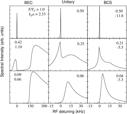
Figure 1: RF spectra $I(\omega)$ for the near-BEC (720 G, left column), unitary (837 G, $k_{F}a=\infty$, middle column), and near-BCS (875 G, right column) cases as a function of RF detuning $\omega$. The values of $T$ (except in the first row) and $k_{F}a$ were chosen to match the experimental values in Ref. Chin et al. (2004).

Figure 1 shows the calculated RF excitation spectra in a harmonic trap for the near-BEC (720 G), unitary (837 G, $a=\infty$) and near-BCS (875 G) cases, from left to right, for a range of $T$ from above to below $T_{c}$. Here, for definiteness, we take $\gamma/E_{F}=0.1+0.3T/T_{c}$, which monotonically increases with $T$ as one may expect Chen et al. (2001). The values of $T$ used in all rows but the first (which involved the less interesting extreme Boltzmann regime) were chosen to be consistent with the corresponding values of $T^{\prime}$ used in Ref. Chin et al. (2004), on the basis of a theoretical thermometry Chen et al. (b). Here $T^{\prime}$ refers to the initial temperature of an isentropic sweep starting from the BEC side of resonance. The values of $k_{F}a$ were calculated from the known values of $T_{F}$ and $a$. Just as in experiment Chin et al. (2004), two distinct maxima are seen. A very sharp peak at $\omega=0$ appears only for $T\neq 0$; this peak is, thus, related to thermally excited fermion states. A second and broader maximum is present at sufficiently low $T$ and is connected to the breaking of fermion pairs between states $|1\rangle$ and $|2\rangle$, with subsequent transfer of state $|2\rangle$ to $|3\rangle$. The broadening of zero $\omega$ peak, as $T$ decreases, reflects the increasing values of the gap $\Delta$. The general features of the spectra are in reasonable agreement with experiment for all three cases shown.

The near-BEC plot is still far from the true BEC limit where $k_{F}a$ is arbitrarily small. Nevertheless, one can see from the lowest $T$ figure that the absorption onset is only slightly larger ($\sim 5E_{F}$ as compared to $\sim 4.6E_{F}$) than the estimated two-body binding energy $\hbar^{2}/ma^{2}$, as expected. This near-BEC figure makes it clear that pairing effects are absent at the highest $T=1.0T_{F}\,\,(\gtrsim T^{*})$, where the free atom peak is symmetric and there is no sign of a shoulder; this case is close to unitarity largely because of the size of $k_{F}$. It is also clear from the middle figure that the “pairing gap” forms above $T_{c}$, as is expected. Although not shown here, we find that for the unitary case, there is an analogous pseudogap effect which appears above $T_{c}$ via a shoulder in the spectra to the right of the $\omega=0$ peak. Only when $T>T^{*}$ will this shoulder entirely disappear. At unitarity, we find $T^{*}\approx 2T_{c}$. Additionally, it should be stressed that the near-BCS case is still very far from the weak coupling BCS limit.

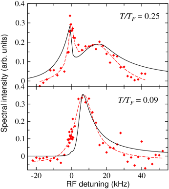
Figure 2: Comparison of calculated RF spectra (solid curve, $T_{c}\approx 0.29$) with experiment (symbols) in a harmonic trap calculated at 822 G for the two lower temperatures. The temperatures were chosen based on Ref. Chin et al. (2004). The particle numbers were reduced by a factor of 2.

Experimentally Bartenstein et al. , one defines the (averaged) “pairing gap”, $\Delta_{RF}$, as the energy splitting between the maximum in the broad RF feature and the $\omega=0$ point. For the near-unitary case in ⁶Li (at 822 G), $\Delta_{RF}/E_{F}\approx 0.25$ at the intermediate $T^{\prime}=0.5T_{F}$, whereas at the lowest $T$ this ratio is around $0.35$. The ratios found theoretically are roughly $0.35$ and $0.38$ for these two cases. However, when the field is increased to precise unitarity (837 G) the numbers appear to considerably smaller with a ratio of $\lesssim 0.2$. On general grounds one can argue that very little change is expected with these small changes in field near unitarity. Anharmonicity associated with a shallow Gaussian trap may explain this small discrepancy, along with possible uncertainties in the particle number pri ; Perali et al. (2004). There may also be some interference with the Feshbach resonances between states $|1\rangle$ and $|3\rangle$ and between $|2\rangle$ and $|3\rangle$ Bartenstein et al. (2005), which overlap with the resonance between $|1\rangle$ and $|2\rangle$ but are not included in the theory.

In Fig. 2, we compare our calculated spectra near unitarity (solid curve) with experiment (symbols) at 822 G for the two lower temperatures. The dashed curve is a fit to the data, serving as a guide to the eye. As in Fig. 1, we calculated $k_{F}a$ using the experimental values of $T_{F}$ and $a$ Bartenstein et al. . After reducing the particle numbers by a factor of 2, as in Ref. Perali et al. (2004), this brings the theory into very good agreement with experiment.

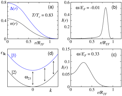
Figure 3: Origin of the two RF spectral peaks. Spatial distribution of (a) $\Delta$ and density $n(r)$, contributions to (b) the low frequency peak at $\omega/E_{F}=-0.01$ and (c) the high frequency peak at $\omega/E_{F}=0.33$ at unitarity in a harmonic trap, calculated at $T=0.23T_{F}$. (d) Schematic transitions from state $|2\rangle$ to $|3\rangle$, showing the extended $k$-space contributions to the low energy peak, at the trap edge where $\Delta<T$. Here $R_{TF}$ is the Thomas-Fermi radius for a noninteracting Fermi gas.

To fully understand the RF excitation spectra, it is important to determine where, within the trap, the two frequency peak features originate. Figure 3(a) shows a plot of the density profile $n(r)$ and excitation gap $\Delta(r)$ at unitarity and $T\approx 0.23T_{F}\approx 0.83T_{c}$ as a function of radius. Figures 3(b) and 3(c) indicate the radial dependence of the local current $I(r,\omega)$ for (b) frequency near zero, where there is a sharp peak, and for (c) frequency near the pairing gap energy scale, where there is a broad peak. Just as conjectured in previous papers Chin et al. (2004); Kinnunen et al. (2004b), it can be seen that the low frequency peak is associated with atoms at the edge of the trap. These are essentially “free” atoms which have very small excitation gap values, so that they are most readily excited thermally. By contrast, the pairing gap peak is associated with atoms somewhere in the middle of the trap.

One might expect a rather broad free atom peak, reflecting a range of values of $\Delta(r)$ at trap edge, but this peak is, in fact, quite sharp, as is its experimental counterpart. The sharpness of the free atom peak is addressed via the schematic diagram of Fig. 3(d). When $\Delta<T$ (as in the trap edge region), the dispersion of state $|2\rangle$ reduces to a simple parabola as for free fermions; it is thus similar to that of state $|3\rangle$, as seen in Fig. 3(d). Momentum conservation leads to vertical transitions shown by the arrows on the figure. It is important to contrast this picture with the situation for SN tunneling; here Pauli blocking effects are absent since the final state is empty for all $\mathbf{k}$. As a result there is an extended volume of $k$-space contributing to the transition at $\omega_{L}=\omega_{23}$ (which corresponds to detuning $\omega=0$), thereby leading to the sharp spectral peak. At the very high $T$ which were probed experimentally in Ref. Chin et al. (2004), the sharp $\omega=0$ peak results in a similar fashion, although in this Boltzmann regime, the gap $\Delta$ is completely irrelevant.

A plot analogous to Figs. 3(b) and 3(c) can be made for the near-BEC case as well, to determine where in the trap the RF gap $\Delta_{RF}$ arises. It is easy to see that the threshold region is associated with the trap edge where $\Delta(r)$ is small. Indeed, when $\mu<0$, the excitation gap is given by $\sqrt{\mu^{2}+\Delta^{2}}$. This implies that the two-body binding energy $E_{b}\approx-2\mu+a\pi n\hbar^{2}/m$ sets the scale for this threshold, in much the same way as found for the deep BEC where $a\rightarrow 0$. As long as $\mu<0$, the values of $\Delta_{RF}$ and $E_{b}$ are very close, becoming equal when $\Delta\rightarrow 0$ at the trap edge. This supports the more detailed two-body analysis of these threshold effects in the BEC presented in Ref. Chin and Julienne (2005). However, it should be stressed that there is an intrinsic rounding around the threshold, as seen in the bottom left panel of Fig. 1.

At $T=0$ these LDA-based RF calculations can be compared with the results Ohashi and Griffin of Bogoliubov-de Gennes (BdG) theory. It should be noted that BdG theory is appropriate for the particular mean field ground state under consideration, but it cannot be applied at $T\neq 0$, since it does not take into account the noncondensed bosonic degrees of freedom. A comparison presented in Ref. Ohashi and Griffin between a BdG calculation and its LDA approximation showed a difference in the low frequency tunneling current at $T=0$ in the fermionic regime ($\mu>0$). The finite spectral weight at precisely $\omega=0$ in the BdG result was interpreted to arise from Andreev bound states Tor .

It was also speculated that at finite $T$, Andreev effects may be playing a role so that the free atom peak is possibly of a different origin from that considered here and elsewhere Chin et al. (2004); Kinnunen et al. (2004b). It was noted in Ref. Ohashi and Griffin that the BdG equations show that the entire trapped gas is in the superfluid state below $T_{c}$, with $\Delta_{sc}(r)$ being finite everywhere $n(r)$ is finite. Therefore, it was presumed that the free atom peak found in Ref. Kinnunen et al. (2004b) was an artifact of the LDA at $T\neq 0$, since in this approximation, there is a region of the trap where $\Delta_{sc}=0$.

In support of the present viewpoint it is important to note that the free atom peak derives from states where $\Delta(r)<T$. The gap $\Delta$, is the important energy scale, not the order parameter $\Delta_{sc}$, for characterizing fermionic single-particle excitations. This can be seen from the fact that the spectral function of Eq. (3) which enters into the RF calculations depends on $\Delta$ through $E_{\bf k}$, and is not particularly sensitive to $\Delta_{sc}$. From Fig. 3(a) it follows that $\Delta$ is finite wherever $n(r)\neq 0$. It behaves similarly to the nonvanishing order parameter in BdG-based calculations. Furthermore, both the OP in Ref. Ohashi and Griffin and $\Delta$ (for the present case) behave as $\Delta\sim\exp(-\pi/2k_{F}|a|)$, becoming exponentially small at the trap edge. Thus, as a result of pseudogap effects (which serve to distinguish $\Delta$ and $\Delta_{sc}$ at any finite $T$) we believe that the concerns raised earlier Ohashi and Griffin about the applicability of LDA for addressing RF experiments are not warranted.

The results of this paper support a previous theoretical interpretation Kinnunen et al. (2004b) of RF experiments Chin et al. (2004) in the unitary regime, which applied the pseudogap based formalism of the present paper, albeit with approximated spatial density and gap profiles. The present calculations avoid these approximations, and lead to spatial density profiles Stajic et al. (2005) and related thermodynamics Kinast et al. (2005) which are in good quantitative agreement with experiment Stajic et al. (2005). Our work clarifies the origin of the two generic peak structures seen in RF experiments, and addresses the entire magnetic field range which has been studied experimentally. The zero frequency peak comes from atoms at the edge of the trap, where $\Delta<T$. We interpret these as “small-gap” rather than “in-gap” excitations. We have shown that the sharpness of this peak is associated with an extended momentum space available for the $\omega=0$ excitations. The broader peak derives from the breaking of pairs and, except in the extreme BCS limit, this peak is present above $T_{c}$, reflecting pseudogap effects.

We are extremely grateful to Cheng Chin, Rudi Grimm and Paivi Törmä for many helpful discussions. This work was supported by NSF-MRSEC Grant No. DMR-0213745 and by the Institute for Theoretical Sciences (University of Notre Dame and Argonne Nat’l Lab), and by DOE, No. W-31-109-ENG-38 (QC).

References

- Regal et al. (2004) C. A. Regal, M. Greiner, and D. S. Jin, Phys. Rev. Lett. 92, 040403 (2004).
- Zwierlein et al. (2004) M. W. Zwierlein et al., Phys. Rev. Lett. 92, 120403 (2004).
- Kinast et al. (2004) J. Kinast et al., Phys. Rev. Lett. 92, 150402 (2004).
- Bartenstein et al. (2004) M. Bartenstein et al., Phys. Rev. Lett. 92, 203201 (2004).
- Chen et al. (a) Q. J. Chen, J. Stajic, S. N. Tan, and K. Levin, arXiv:cond-mat/0404274; To appear in Physics Reports.
- Stajic et al. (2004) J. Stajic et al., Phys. Rev. A 69, 063610 (2004).
- Chin et al. (2004) C. Chin et al., Science 305, 1128 (2004).
- Greiner et al. (2005) M. Greiner, C. A. Regal, and D. S. Jin, Phys. Rev. Lett. 94, 070403 (2005).
- Törmä and Zoller (2000) P. Törmä and P. Zoller, Phys. Rev. Lett. 85, 487 (2000).
- Kinnunen et al. (2004a) J. Kinnunen, M. Rodriguez, and P. Törmä, Phys. Rev. Lett. 92, 230403 (2004a).
- Kinnunen et al. (2004b) J. Kinnunen, M. Rodriguez, and P. Törmä, Science 305, 1131 (2004b).
- (12) Y. Ohashi and A. Griffin, arXiv:cond-mat/0410220.
- Stajic et al. (2005) J. Stajic, Q. J. Chen, and K. Levin, Phys. Rev. Lett. 94, 060401 (2005).
- Kinast et al. (2005) J. Kinast, A. Turlapov, J. E. Thomas, Q. J. Chen, J. Stajic, and K. Levin, Science 307, 1296 (2005).
- O’Hara et al. (2002) K. M. O’Hara et al., Science 289, 2179 (2002).
- Chen et al. (b) Q. J. Chen, J. Stajic, and K. Levin, arXiv:cond-mat/0411090.
- Leggett (1980) A. J. Leggett, in Modern Trends in the Theory of Condensed Matter (Springer-Verlag, Berlin, 1980), pp. 13–27.
- Timmermans et al. (2001) Timmermans et al., Phys. Lett. A 285, 228 (2001).
- Chen et al. (2001) Q. J. Chen, K. Levin, and I. Kosztin, Phys. Rev. B 63, 184519 (2001).
- (20) Bartenstein et al., arXiv:cond-mat/0412712.
- (21) C. Chin, private communications.
- Perali et al. (2004) A. Perali, P. Pieri, and G. C. Strinati, Phys. Rev. Lett. 93, 100404 (2004).
- Bartenstein et al. (2005) Bartenstein et al., Phys. Rev. Lett. 94, 103201 (2005).
- Chin and Julienne (2005) C. Chin and P. Julienne, Phys. Rev. A 71, 012713 (2005).
- (25) Törmä has suggested that the BdG calculations based on a small particle number and a narrow Feshbach resonance may not be directly comparable to the LDA calculations even at .