Measurement of Counting Statistics of Electron Transport in a Tunnel Junction

Abstract

We present measurements of the time-dependent fluctuations in electrical current in a voltage-biased tunnel junction. We were able to simultaneously extract the first three moments of the tunnel current counting statistics. Detailed comparison of the second and the third moment reveals that counting statistics is accurately described by the Poissonian distribution expected for spontaneous current fluctuations due to electron charge discreteness, realized in tunneling transport at negligible coupling to environment.

Photon counting statistics MandelWolf ; WallsMilburn is a key technique of quantum optics, which is routinely used to study temporal and spectral distribution of electromagnetic field, and to characterize the complexity of optical states, such as photon coherence, entanglement, and squeezing. In contrast, the electron counting and noise statistics, which are expected to provide new insights into quantum transport, is essentially at infancy as experimental subject, with the first advances made only recently Reulet1 ; Rimberg ; Fujisawa ; Delsing ; ReuletPRL .

Electron counting proves to be far more challenging than that of photons primarily because of the extremely high frequency of electron passage events at typical current intensity, which requires fast charge detection. While in some cases Coulomb blockade in quantum dots can be used to localize electrons and suppress tunneling, bringing the tunneling frequency down to the radio frequency range Rimberg ; Fujisawa ; Delsing , the time resolution needed to measure free, nonlocalized electrons remains a challenge.

Another difficulty stems from the simple fact that, while photons do not interact, the electrons do. The electric field fluctuations produced by the electrons which are being measured can propagate out to other parts of the circuit (‘environment’) and perturb it. In turn, the noise due to the environment, modulated by the signal, can couple back to the region of interest, strongly affecting the measured signal KNB02 ; Nagaev02 ; Beenakker03 ; Reulet1 ; ReuletPRL ; Geneva_group ; Gutman05 .

The electron problem is especially rich and intriguing: unlike photons, the current fluctuations are measured without extracting electrons out of the system. The electrons remain part of the many-body system while being detected, allowing quantum phenomena to fully manifest themselves in electric noise. This leads to a number of dramatic effects observed in electric noise, such as, notably, elementary charge transmutation in the Fractional Quantum Hall effect depicciotto97 ; glattli97 ; reznikov99 and charge doubling in the Andreev scattering regime in NS junctions Kozhevnikov2000 .

The regime in which electric fluctuations occur spontaneously due to charge discreteness, rather than due to thermal fluctuations, is realized at sufficiently low temperatures lesovik89 ; khlus87 ; BlanterReview . It was first demonstrated about 10 years ago in semiconductor point contacts reznikov95 ; kumar96 and in mesoscopic wires martinis96 ; schoelkopf97 . Current fluctuations in this regime are traditionally analyzed using the noise frequency spectrum. However, a more detailed descriptionlevitov93 ; Nazarov03 is provided by the statistics of the charge $q(\tau)$ transmitted through a conductor during a fixed time interval $\tau$ which, in principle, can be small or large compared to the time $\tau_{0}=e/I$. The low frequency shot noise is just the second central moment of the transmitted charge distribution $P(q)$ at long times $\tau\gg\tau_{0}$:

$$S^{(2)}=\langle I_{\omega}^{\ast}I_{\omega}\rangle_{\omega=0}=\frac{\langle\Delta q^{2}(\tau)\rangle}{\tau}=\frac{\langle(q(\tau)-\bar{q})^{2}\rangle}{\tau}$$ (1)

with $\langle...\rangle$ a shorthand for $\int...P(q,\tau)dq$. The counting distribution $P(q)$, which encodes the full information about noise statistics, was studied in various regimes, including mesoscopic scattering levitov93 , photon-assisted transport ivanov93 , and transport in NS junctions muzykantskii ; nazarovNS , where charge doubling takes place. Specifics of the tunneling regime were considered in LR01 ; sukhorukov .

The present work extends the shot noise measurements beyond the second moment in a way uncorrupted by the presence of electromagnetic environment. The results agree with the expectation for Poisson process, thus paving the way to investigation of counting statistics. We measure current fluctuations in a tunnel junction by detecting the probability distribution of voltage across a load resistor, $P(V)$. The latter is directly related to $P(q)$ when the load resistance is made much smaller than the tunnel resistance. The knowledge of $P(q)$ allows, in principle, to obtain all moments of $q$. However, with the measurement times $\tau\gg\tau_{0}$, due to the central limit theorem, the high moments become increasingly dominated by the lower order moments. This makes the irreducible parts of the moments, the cumulants, which contain new information, increasingly difficult to extract. Thus here we shall focus on the third central moment $\langle\Delta q^{3}\rangle=\langle(q-\bar{q})^{3}\rangle$ which coincides with the third cumulant $\langle\!\langle q^{3}\rangle\!\rangle$.

The expected statistics is different in the voltage-biased and current-biased regimes. The former case is described by the rate of the attempts to pass equal to $eV/h$ and a binomial distribution of successes levitov93 . At weak transmission, realized in tunnel junction, the distribution assumes Poisson form, with the low frequency spectral density $S^{(k)}$ of the $k$-th cumulant, corresponding to the ‘long’ measurement time $\tau\gg\tau_{0}$, expressed as

$$S^{(k)}=\frac{\langle\!\langle q^{k}\rangle\!\rangle}{\tau}=e^{k-1}I$$ (2)

In contrast, in a current-biased sample, the rate of successes is fixed at $I/e$, and the attempts to pass, described by fluctuating time-dependent voltage across the sample, are characterized by Pascal distribution KNB02 . A general cascade approach to high-order noise statistics in the diffusive regime was developed in Ref. Nagaev02 , the role of external circuit was considered in Ref. Beenakker03 (see also Geneva_group ).

In the first measurement of the third moment $S^{(3)}$ Reulet et al. Reulet1 ; ReuletPRL used a low impedance tunnel junction ($R_{s}\simeq 50$ Ohm) as a noise source, with a parallel $50$ Ohm load impedance $R_{l}$ of the cable used to feed the voltage to an external amplifier. The initial results Reulet1 distinct difference from the Poissonian, in both magnitude and sign, suggested that $S^{(3)}$ is dominated by the effects extraneous to the junction. A theoretical investigation KNB02 ; Beenakker03 followed which clarified the importance of the external circuit for correct interpretation of the results, obtaining the third moment of the form

$$S^{(3)}=S_{s}^{(3)}-3R_{s,l}(S_{s}^{(2)}+S_{l}^{(2)})\frac{\partial(S_{s}^{(2)}-S_{l}^{(2)})}{\partial V}$$ (3)

with $R_{s,l}=R_{s}R_{l}/(R_{s}+R_{l})$ the impedance of the sample in parallel with the load, $S_{s}^{(2)}$ and $S_{l}^{(2)}$ the sample and load noise, and $S_{s}^{(3)}$ generated by the voltage-biased sample. The load resistor, being macroscopic, is not expected to produce a third cumulant Nagaev02 ; BlanterReview . The measurement Reulet1 ; ReuletPRL , which due to $R_{l}\simeq R_{s}$ was neither fully in the voltage-, nor in the current-biased regime, was dominated by the voltage-dependent $S_{s}^{(2)}$ in the last term of Eq.(3). Only at room temperature, due to low $\partial S_{s}^{(2)}/\partial V$, the result had the sign of $S_{s}^{(3)}$.

To measure the intrinsic $S^{(3)}$ free of the admixture of the second moment, we use a new method suggested and analyzed in Ref.LR01 (Fig.1). Current fluctuations generated by the sample (voltage-biased tunnel junction of high impedance) produce voltage fluctuations on the load resistor $R_{l}$ which are amplified and analyzed with computer. The statistics of voltage fluctuations on $R_{l}$ is identical to that of the intrinsic current fluctuations in the junction, provided that $R_{l}$ is much smaller than the junction differential resistance.

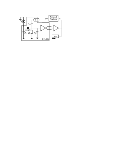
Figure 1: Schematic of the experimental setup. The current source drives constant average current $I$ while the capacitor $C_{v}$ fixes the voltage across the sample and the load at relevant frequencies. The bandwidth is determined by the load resistance $R_{l}$ and stray capacitance $C_{s}$. The voltage fluctuations across the load resistor are amplified and digitized by a 12 bit analog-to-digital convertor (A/D) obtained from Ultraview Corp. with 5 ns sampling time and 20 ns interval between the samples. The amplifier input impedance is determined by $R_{l}$.

The main source of errors in the measurement of the $k$-th cumulant $\langle\!\langle q^{k}\rangle\!\rangle$ of the distribution $P(q)$ is statistical. In order to estimate the signal-to-noise ratio the measured value $\langle\!\langle q^{k}\rangle\!\rangle$ should be compared to its variance ${\rm var}(\Delta q^{k})$ due to both sample and amplifier noise. The variance is expressed through the central moments of the order $2k$. The variance of an even order for a generic distribution can be estimated with the help of the central limit theorem, using Gaussian statistics:

$${\rm var}(\Delta q^{k})=\left(\langle\Delta q^{2k}\rangle\right)^{1/2}\simeq\left((2k-1)!!\right)^{1/2}\langle\Delta q^{2}\rangle^{k/2}$$ (4)

Here the variance $\langle\Delta q^{2}\rangle$ in Eq.(4) is due to the sample, amplifier and load noise, $S^{(2)}=S^{(2)}_{s}+S^{(2)}_{l}+S^{(2)}_{a}$, assuming all three to be uncorrelated. The signal-to-noise ratio for a single measurement of the third cumulant is thus estimated as a ratio of $S_{3}\tau$ to $15^{1/2}(S_{2}\tau)^{3/2}$, and therefore it is beneficial to reduce the sampling time $\tau$ to improve sensitivity, in accord with the central limit theorem. However, the amplified signal is correlated at short times due to finite bandwidth of the input circuit. This makes the effective sampling time restricted from below by the sample parasitic capacitance, $C_{s}$, of both intrinsic and stray kind, and by the effective output resistance of the sample in parallel with the load resistance of the amplifier, $R_{l}$, so that $\tau_{\rm eff}\simeq R_{l}C_{s}$. Repeating the measurement $N$ times would further reduce fluctuations by a factor $\sqrt{N}$, assuming statistically independent successive measurements. However, since the measurements separated in time by less than $\tau_{\rm eff}$ are correlated, the maximal improvement is of the order of $\sqrt{{\cal T}/\tau_{\rm eff}}$, where $\cal T$ is the measurement time. In the case of a high impedance tunnel junction, the noise is dominated by the resistor $R_{l}$ thermal noise, $2k_{B}T/R_{l}$. The measurements were performed at 4.2 K to reduce both this noise and the noise of the amplifier. Ignoring for now both the shot noise produced by the sample and the amplifier noise, we estimate the signal-to-noise ratio as

$$S/N=\frac{e^{2}I\sqrt{\cal T}}{\sqrt{15}(2k_{B}T/R_{l})^{3/2}\sqrt{\tau\tau_{\rm eff}}}$$ (5)

Replacing $\tau$ by $\tau_{\rm eff}$ and plugging in Eq.(5) we find the signal-to-noise ratio $S/N\propto R_{l}^{1/2}C_{s}^{-1}$. It is therefore clear that it pays to decrease $C_{s}$ and increase $R_{l}$ to improve $S/N$. We placed a cold amplifier in the vicinity of the sample to reduce as much as possible the capacitance $C_{s}$. The choice of the $R_{l}$ is restricted by the desire to keep most of the signal at frequencies well above $1/f$ corner of the amplifier. We chose $R_{l}=9.1\,{\rm kOhm}$ which together with the stray capacitance of about $4\,{\rm pF}$ gives $\tau_{\rm eff}=R_{l}C_{s}\simeq 40\,{\rm ns}$ and signal bandwidth $(2\pi\tau_{\rm eff})^{-1}\approx 4\,{\rm MHz}$. To keep the sample under voltage bias, we introduced a capacitor $C_{v}$ which kept the voltage constant across the sample-load circuit at all relevant frequencies.

We used tunneling through a $30{\rm{\AA}}$ thick ${\rm SiO_{2}}$ gate oxide of a $p$-channel Si field-effect transistor to produce a shot noise. In this system tunneling occurs only under negative gate voltage required to induce a hole channel. The differential resistance of the barrier $R_{s}=(\partial I/\partial V)^{-1}>10^{7}\ {\rm Ohm}$ was much bigger then $R_{l}$, placing the sample securely in the voltage-biased regime. Indeed, the maximal contribution of the second term in Eq.(3),

$$-3Z(eI+2k_{B}T/R_{l})e\frac{\partial I}{\partial V}\approx-\frac{6ek_{B}T}{(R_{l}+R_{s})},$$ (6)

is estimated as $5.2\times 10^{-48}\ {\rm A^{3}/Hz^{2}}$, which is two orders of magnitude smaller then $e^{2}I$ (Fig. 3).

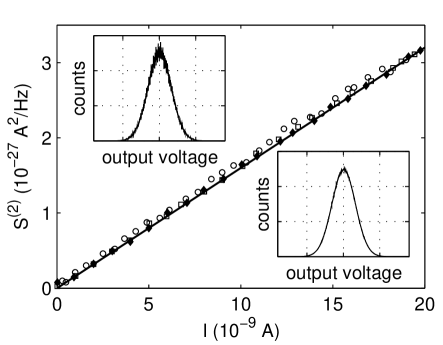
Figure 2: Measured value of the noise, $S^{(2)}$, as a function of the current. Different markers represent the data of three different measurements. The straight line $S^{(2)}=eI$, corresponding to the expected noise intensity factor2 , is shown for guidance. Upper inset: raw voltage histogram sample; Lower inset: cleaned histogram, illustrating the result of normalizing with the A/D converter calibration (see text).

Figure 3: Measured third cumulant $S^{(3)}$ of the transmitted charge, obtained separately for different current directions. (Markers are the same as in Fig. 2, the straight line is $S^{(3)}=e^{2}I$.) Upper inset: $S^{(3)}$ vs. $I$ without amplifier nonlinearity correction; Lower inset: normalized histogram of the linearly swept signal, used to calibrate the A/D converter (see text).

We record the probability distribution function $P(V_{a})$ of the amplified voltage $V_{a}$ (Fig. 2, upper inset). To clean the obtained histogram we correct for nonequal bin widths of the A/D converter by calibrating the latter against linearly swept signal (Fig. 3, lower inset). The effect of normalizing $P(V_{a})$ with the A/D converter calibration, illustrated in Fig. 2 lower inset, is two-fold. First, the histogram loses the erratic features (‘grass’) on the smallest scale. Simultaneously, the envelope is somewhat corrected on large scale. The latter effect, due to averaging, has longer stability time, which is fortunate, since the ‘grass’ features, while less stable, were found to have little effect on the second and the third cumulant.

For a linear circuit, the amplified voltage $V_{a}(\omega)$ and the input current $i(\omega)$ Fourier components are proportional: $V_{a}(\omega)=Z(\omega)K(\omega)i(\omega)$, with $Z$ the load impedance and $K$ the amplification. Therefore the third cumulant is related to the respective spectral densities of $V_{a}$ as

$$\langle V_{a}^{(3)}\rangle=\frac{S^{(3)}}{(2\pi)^{2}}{\iint}_{-\infty}^{+\infty}A(\omega)A(\omega^{\prime})A(-\omega-\omega^{\prime})d\omega d\omega^{\prime}$$ (7)

with $A(\omega)=Z(\omega)K(\omega)$. For the broadband amplifiers used, the amplification $K(\omega)$ was almost frequency independent between the low $\sim 0.5\ {\rm MHz}$ and high $\sim 25\ {\rm MHz}$ frequency cutoffs intentionally introduced to filter the $1/f$ amplifier noise and the wide-band noise at frequencies well above $(2\pi\tau_{\rm eff})^{-1}$. The complex product $Z(\omega)K(\omega)$ was obtained from calibration, introducing a known current through a small capacitor $C_{c}$ typically of 2.4 pF. We then used Eq.(7) for $V_{a}^{(3)}$ and a similar expression for $V_{a}^{(2)}$ to extract $S^{(3)}$ and $S^{(2)}$. The second cumulant $S^{(2)}$ combines the shot, thermal and amplifier noise contributions. Since only the former depends on current, the amplifier noise and the thermal noise, obtained from $S^{(2)}$ at zero current, can be easily subtracted CurrNoise . The resulting noise $S^{(2)}$, shown in Fig. 2, varies linearly with current as expected ($eV\simeq 4\,{\rm V}\gg k_{B}T$ at all currents). The measured value agrees with the expected value, $eI$, within calibration error of 5%.

In order to extract properly the third cumulant of the voltage, one should account for the effect of amplification nonlinearity which can mix $S^{(2)}$ with $S^{(3)}$. Let us consider the amplifier nonlinearity, $V_{out}=K(V_{in}+V_{in}^{2}/U)$, with $1/U$ the nonlinearity parameter, which which contributes to the cumulants $\langle\delta V_{out}^{2}\rangle$ and $\langle\delta V_{out}^{3}\rangle$ as follows:

$$\langle\delta V_{out}^{2}\rangle/K^{2}-\langle\delta V_{in}^{2}\rangle=2\langle\delta V_{in}^{3}\rangle/U+3\langle\delta V_{in}^{2}\rangle^{2}/U^{2}$$ (8)

$$\langle\delta V_{out}^{3}\rangle/K^{3}-\langle\delta V_{in}^{3}\rangle=9\langle\delta V_{in}^{2}\rangle^{2}/U$$ (9)

The right hand side of the Eq.(9) would affect the value $S^{(3)}$ calculated from $\langle\delta V_{out}^{3}\rangle$. The parameter $U$ can be estimated by applying an ac signal and measuring its second harmonic. We took special care to reduce nonlinearity of the amplifier track, especially the last amplifier in the chain. We managed to make it comparable to the nonlinearity of the cryogenic amplifier which was different for different measurements, depending on the regime. We found $U$ to exceed $20\,{\rm mV}$, and thus having negligible effect on $S^{(2)}$. However, estimates show that the nonlinearity correction to $S^{(3)}$ can be as large as $10^{-45}\,{\rm A^{3}/Hz^{2}}$. We attribute the third cumulant at zero current (see the upper inset of Fig. 3) to this nonlinearity and determine $U$ as the ratio $9\langle\delta V_{in}^{2}\rangle^{2}_{I=0}/\langle\delta V_{out}^{3}\rangle_{I=0}$. Using this $U$ we subtract the nonlinearity contribution, Eq.(9), from the data at all currents. This procedure, as illustrated in Fig. 3 upper inset, restores zero value at $I=0$, but has little effect on the slope of the dependence $S^{(3)}$ vs. $I$. We therefore conclude that the nonlinearity, while necessary to account for to improve accuracy, is not strong enough to compromise the measurement of $\partial S^{(3)}/\partial I$. The results, shown in Fig. 3, are found to be in excellent agreement with the Poissonian third cumulant $e^{2}I$.

As an additional check, we also reversed the current direction. Since we had to apply negative voltage on the gate to induce holes, it required rebonding the sample (see Fig. 3, upper inset). We found the third cumulant to be an odd function of current, as expected.

Note added: Finally, we note that the literature is not entirely unanimous regarding the Poissonian character of tunneling transport. Dissent is exemplified by Ref. Lesovik03 , predicting a new ”quantum regime” at sufficiently low frequencies, limited by inverse flight time in a noninteracting fermion model. Ref. Lesovik03 obtains $S^{(3)}$ for the tunneling current of sign opposite to Poissonian $S^{(3)}$ and also of much smaller magnitude, quadratic in transmission rather than linear as in Eq.(2) above. The conditions stated in Ref. Lesovik03 are fulfilled in our experiment: the time interval between electron tunneling and its detection, estimated from EM signal propagation speed, is of order $3\cdot 10^{-11}\,{\rm s}$, which is much shorter than the sampling time, $5\,{\rm ns}$, placing the measurement securely at low frequency in the sense of Ref. Lesovik03 . The results Lesovik03 are thus not in accordance with our observations.

In summary, we present the first measurements of the charge counting statistics in voltage-biased tunnel junction up to the third cumulant. The results, obtained by analyzing the distribution of transmitted charge, are in excellent agreement with expectations for Poissonian process, making electron counting statistics amenable to experimental investigation.

We are indebted to O. Prus for his contribution at the early stage of the work. One of us (M.R.) is indebted to G. Lesovik for attracting his attention to the problem. This research was supported by the US-Israel Binational Science Foundation and (D.S. and Yu. B.) by the Lady Davis Fellowship.

References

- (1) L. Mandel and E. Wolf, Optical Coherence and Quantum Optics, Cambridge University Press (Cambridge, 1995).
- (2) D. Walls, G. J. Milburn, Quantum Optics, Springer-Verlag (New York, 1995).
- (3) B. Reulet, J. Senzier, and D. E. Prober, contribution to the International Workshop “Electrons in Zero-Dimensional Conductors,” Max Planck Institute for the Physics of Complex Systems, Dresden, 2002; condmat/0302084v1.
- (4) Lu Wei, Ji ZhingQing, L. Pfeiffer, K.W. West and A.J. Rimberg, Nature (London) 423, 422 (2003).
- (5) T. Fujisawa, T. Hayashi, Y. Hirayama, H. D. Cheong and Y. H. Jeong, Appl. Phys. Lett., 84, 2343 (2004).
- (6) J. Bylander, T. Duty and P. Delsing, Nature (London) 434, 361 (2005).
- (7) B. Reulet, J. Senzier and D. E. Prober, Phys. Rev. Let. 91, 196601 (2003).
- (8) K.E. Nagaev, Phys. Rev. B66, 075334 (2002).
- (9) M. Kindermann, Yu. V. Nazarov, C. W. J. Beenakker Phys. Rev. Lett. 90, 246805 (2003).
- (10) C. W. J. Beenakker, M. Kindermann, and Yu. V. Nazarov, Phys. Rev. Let. 90, 176802 (2003).
- (11) S. Pilgram, A. N. Jordan, E. V. Sukhorukov, M. Buttiker, Phys. Rev. Lett. 90, 206801 (2003); cond-mat/0212446; A. N. Jordan, E. V. Sukhorukov, S. Pilgram, J. Math. Phys. 45, 4386 (2004); cond-mat/0401650;
- (12) D.B. Gutman, A.D. Mirlin, and Y. Gefen, Phys. Rev. B 71, 085118 (2005).
- (13) R. de-Picciotto, M. Reznikov, M. Heiblum, V. Umansky, G. Bunin and D. Mahalu, Nature (London) 389, 162 (1997).
- (14) L. Saminadayar, D. C. Glattli, Y. Jin and B. Etienne, Phys. Rev. Lett. 79, 2526 (1997).
- (15) M. Reznikov, R. de Picciotto, T. G. Griffiths, M. Heiblum, and V. Umansky, Nature (London) 399, 238 (1999).
- (16) A. A. Kozhevnikov, R. J. Schoelkopf, and D. E. Prober, Phys. Rev. Lett. 84, 3398 (2000).
- (17) G. B. Lesovik, JETP Lett. 49, 592 (1989).
- (18) V. K. Khlus, Sov. Phys. JETP 66, 1243 (1987).
- (19) Y.M. Blanter and M. Büttiker, Phys. Rep. 336, 1 (2000).
- (20) M. Reznikov, M. Heiblum, Hadas Shtrikman and D. Mahalu, Phys. Rev. Lett. 75, 3340 (1995).
- (21) A. Kumar, L. Saminadayar, D. C. Glattli, Y. Jin and B. Etienne, Phys. Rev. Lett. 76, 2778 (1996).
- (22) A. H. Steinbach, J. M. Martinis, M. H. Devoret, Phys. Rev. Lett. 76, 3806 (1996).
- (23) R. J. Schoelkopf, P. J. Burke, A. A. Kozhevnikov, D. E. Prober, M. J. Rooks, Phys. Rev. Lett. 78, 3370 (1997).
- (24) L. S. Levitov, G. B. Lesovik, JETP Lett. 58, 230 (1993).
- (25) Quantum Noise in Mesoscopic Systems, ed. Yu. V. Nazarov (Kluwer, 2003).
- (26) D. A. Ivanov, L. S. Levitov, JETP Lett. 58, 461 (1993).
- (27) B. A. Muzykantskii, D. E. Khmelnitskii, Phys. Rev. B50, 3982 (1994).
- (28) W. Belzig, Yu. V. Nazarov, Phys. Rev. Lett. 87, 067006 (2001).
- (29) L. S. Levitov, M. Reznikov, Phys. Rev. B70, 115305 (2004), cond-mat/0111057.
- (30) E. V. Sukhorukov, D. Loss, in Electronic Correlations: From meso- to nano-physics, eds. G. Montambaux and T. Martin, XXXVI Rencontres de Moriond (2001), cond-mat/0106307.
- (31) Our definition of noise moments differs by a factor of from the one based on the positive frequency representation for the noise power spectrum. It seems more natural to use the entire range of frequencies from to , which brings the Schottky relation to the form .
- (32) Since the sample differential resistance is much bigger then the load , the resistance seen by the amplifier is current-independent and thus the amplifier current noise contribution is negligible.
- (33) G. B. Lesovik and N. M. Chtchelkatchev, JETP Lett. 77, 393 (2003); cond-mat/0303024