New address: ] IEMN (CNRS-UMR 8520), B. P. 60069, 59652 Villeneuve d’Ascq Cedex, France

Raman spectra of BN-nanotubes: Ab-initio and bond-polarizability model calculations

Abstract

We present ab-initio calculations of the non-resonant Raman spectra of zigzag and armchair BN nanotubes. In comparison, we implement a generalized bond-polarizability model where the parameters are extracted from first-principles calculations of the polarizability tensor of a BN sheet. For light-polarization along the tube-axis, the agreement between model and ab-initio spectra is almost perfect. For perpendicular polarization, depolarization effects have to be included in the model in order to reproduce the ab-initio Raman intensities.

Besides its success in the characterization of a large range of materials cardona , Raman spectroscopy has also developed into an invaluable tool for the characterization of nanotubes. Since the first characterization of (disordered) carbon nanotube (CNT) samples rao97 , the technique has been refined, including, e.g., polarized Raman studies of aligned nanotubes rao00 and isolated tubes due00 . On the theoretical side, non-resonant Raman intensities of CNTs have been calculated within the bond-polarizability model sai98 ; dressbook1 . The empirical parameters of this model are adapted to fit experimental Raman intensities of fullerenes and hydrocarbons. However, the transferability of the parameters and the quantitative performance in nanotubes, in particular distinguishing between metallic and semiconducting tubes, is still not clear.

In this communication, we report on the Raman spectra of boron nitride nanotubes (BNNTs) rub94 ; cho95 . Recently, synthesis of BNNTs in gram quantities has been reported lee01 . Their characterization through Raman and infrared spectroscopy is expected to play an important role. However, due to difficulties with the sample purification no experimental data on contamination-free samples has been reported. Ab-initio  wir03 and empirical san02 ; pop03 phonon calculations have determined the position of the peaks in the spectra. However, due to missing bond-polarizability parameters for BN, the Raman intensities have been so far addressed using the model bond-polarizability parameters of carbon pop03 . Only the intensities of high-frequency modes was presented as it was argued that the intensity of low frequency modes are very sensitive to the bond-polarizability values pop03 . Here, we derive the polarizability parameters for BN sp² bonds from a single hexagonal BN sheet by calculating the polarizability-tensor and its variation under deformation. We compare the resulting spectra for BNNTs with full ab-initio calculations. We derive conclusions about the general applicability of the bond polarizability model for semiconducting CNTs.

In non resonant first-order Raman spectra, peaks appear at the frequencies $\omega_{\nu}$ of the $\nu$ optical phonon with null wave vector with intensities $I^{\nu}$ which in the Placzek approximation cardona are

$$I^{\nu}\propto\left|{\bf e}_{i}\cdot{\bf A}^{\nu}\cdot{\bf e}_{s}\right|^{2}\frac{1}{\omega_{\nu}}(n_{\nu}+1)\;.$$ (1)

Here ${\bf e}_{i}$ (${\bf e}_{s}$) is the polarization of the incident (scattered) light and $n_{\nu}=[\exp(\hbar\omega_{\nu}/k_{B}T)-1]^{-1}$ with $T$ being the temperature. The Raman tensor ${\bf A}^{\nu}$ is

$$A_{ij}^{\nu}=\sum_{\gamma}B_{ij}^{k\gamma}\frac{w_{k\gamma}^{\nu}}{\sqrt{M_{\gamma}}},$$ (2)

where $w_{k\gamma}^{\nu}$ is the $k$th Cartesian component of atom $\gamma$ of the $\nu$th orthonormal vibrational eigenvector and $M_{\gamma}$ is the atomic mass.

$$B_{ij}^{k\gamma}=\frac{\partial^{3}\mathcal{E}}{\partial E_{i}\partial E_{j}\partial u_{k\gamma}}=\frac{\partial\alpha_{ij}}{\partial u_{k\gamma}},$$ (3)

where $\mathcal{E}$ is the total energy of the unit cell, ${\bf E}$ is a uniform electric field and $u_{k\gamma}$ are atomic displacements. This is equivalent to the change of the electronic polarizability of a unit cell, $\alpha_{ij}=\Omega\chi_{ij}$ (where $\Omega$ is the unit cell volume and $\chi_{ij}$ the electric susceptibility), upon the displacement $u_{k\gamma}$. The phonon frequencies and eigenvectors wir03 are determined by density functional perturbation theory bar01 as implemented in Ref. abinit . For the determination of the derivative tensor $B_{ij}^{k\gamma}$ we proceed in two ways: i) we calculate it from first principles using the approach of Ref. laz03, , ii.) we develop a generalized bond-polarizability model.

The basic assumption of the bond polarizability model wol41 ; cardona ; uma01 is that the total polarizability can be modeled in terms of single bond contributions. Each bond is assigned a longitudinal polarizability, $\alpha_{l}$, and a polarization perpendicular to the bond, $\alpha_{p}$. Thus, the polarizability contribution $\alpha_{ij}^{b}$ of a particular bond $b$ is

$$\alpha_{ij}^{b}=\frac{1}{3}(2\alpha_{p}+\alpha_{l})\delta_{ij}+(\alpha_{l}-\alpha_{p})\left(\hat{R}_{i}\hat{R}_{j}-\frac{1}{3}\delta_{ij}\right),$$ (4)

where $\hat{R}$ is a unit vector along the bond. The second assumption is that the bond polarizabilities only depend on the bond length $R$. This allows the calculation of the derivative with respect to atomic displacement, $\partial\alpha_{ij}^{b}/\partial u_{k\gamma}$, in terms of four parameters $\alpha_{l}(R)$, $\alpha_{p}(R)$, $\alpha_{l}^{\prime}(R)$, and $\alpha_{p}^{\prime}(R)$ (see, e.g. Ref. uma01, ). The use of only one perpendicular parameter $\alpha_{p}$ implicitly assumes cylindrical symmetry of the bonds. That can be justified in a sp³ bonding environment. However, in the highly anisotropic environment in a sheet of sp² bonded carbon or BN and the corresponding nanotubes this assumption seems hardly justified. In our model we therefore define a generalized polarizability with an in-plane ($\alpha_{pi}$) and out-of-plane value ($\alpha_{po}$) of $\alpha_{p}$.

With the larger set of parameters, the polarizability tensor takes on the more general form

$$\alpha_{ij}^{b}=\alpha_{l}\hat{R}_{i}\hat{R}_{j}+\alpha_{pi}\hat{S}_{i}\hat{S}_{j}+\alpha_{po}\hat{T}_{i}\hat{T}_{j},$$ (5)

where $\hat{\bf S}$ is a unit-vector pointing perpendicular to the bond in plane, and $\hat{\bf T}$ pointing perpendicular to the bond out of plane. (In the case of $\alpha_{pi}=\alpha_{po}$, Eq. (5) simplifies to Eq. (4) due to the relation $\hat{S}_{i}\hat{S}_{j}+\hat{T}_{i}\hat{T}_{j}=\delta_{ij}-\hat{R}_{i}\hat{R}_{j}$.) For the derivative tensor (of a single bond), we obtain

$$\frac{\partial\alpha_{ij}^{b}}{\partial u_{k\gamma}} = \alpha_{l}^{\prime}\hat{R}_{i}\hat{R}_{j}\hat{R}_{k}+\alpha_{l}((\partial_{k}\hat{R}_{i})\hat{R}_{j}+\hat{R}_{i}(\partial_{k}\hat{R}_{j}))$$ (6)

$$+ \alpha_{pi}^{\prime}\hat{S}_{i}\hat{S}_{j}\hat{R}_{k}+\alpha_{pi}((\partial_{k}\hat{S}_{i})\hat{S}_{j}+\hat{S}_{i}(\partial_{k}\hat{S}_{j}))$$

$$+ \alpha_{po}^{\prime}\hat{T}_{i}\hat{T}_{j}\hat{R}_{k}+\alpha_{po}((\partial_{k}\hat{T}_{i})\hat{T}_{j}+\hat{T}_{i}(\partial_{k}\hat{T}_{j})).$$

The total derivative tensor $B_{ij}^{k\gamma}$ is then just the sum over all $\partial\alpha_{ij}^{b}/\partial u_{k\gamma}$ of all bonds of the system. The orientation of the plane at the position of a particular atom is thereby defined by the three nearest neighbor atoms.

	R (Å)	$\alpha_{l}$ (Å3)	$\alpha_{p}$ (Å3)	$\alpha_{l}^{\prime}$ (Å2)	$\alpha_{p}^{\prime}$ (Å2)
			$\alpha_{pi}$: 0.28		$\alpha_{pi}^{\prime}$: 6.60
BN-sheet	1.44	3.31	$\alpha_{po}$: 0.44	1.03	$\alpha_{po}^{\prime}$: 0.77
c-BN	1.56	1.58	0.42	4.22	0.90
diamond	1.53	1.69	0.71	7.43	0.37

Table 1: Parameters of the bond polarizability model extracted from ab-initio calculations (see text).

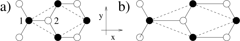
Figure 1: Unit cell (marked by dashed line) of BN-sheet for the calculation of the bond polarizability parameters: a) equilibrium geometry, b) geometry with one bond elongated.

In order to determine the six parameters of our model, we perform ab-initio calculations of the polarizability tensor $\alpha_{ij}$ of a unit-cell of a single BN-sheet distnote ; claus1dim (see Fig. 1 a). The geometry of the system leads to the relations $\alpha_{xx}=\alpha_{yy}=(3/2)(\alpha_{l}+\alpha_{pi})$ and $\alpha_{zz}=3\alpha_{po}$ (with the z-axis perpendicular to the sheet). Displacing atom 2 in $y$-direction yields the relation $\partial\alpha_{xx}/\partial u_{2y}=(3/4)(\alpha_{l}^{\prime}+\alpha_{pi}^{\prime})+(3/2)(\alpha_{l}+\alpha_{pi})/R$. Finally, by changing the geometry of the unit-cell such that one bond is elongated while the other two bond-lengths and all the bond angles are kept constant (see Fig. 1 b), we extract the derivatives of the bond polarizabilities: $\alpha_{l}^{\prime}=\alpha_{xx}^{\prime}$, $\alpha_{pi}^{\prime}=\alpha_{yy}^{\prime}$, and $\alpha_{po}^{\prime}=\alpha_{zz}^{\prime}$. The resulting parameters are displayed in Tab. I and compared to the parameters we calculated for cubic BN and diamond. The longitudinal bond polarizability $\alpha_{l}$ is considerably larger than $\alpha_{p}$ which can be intuitively explained as a consequence of the “enhanced mobility” of the electrons along the bond. For the sheet, the perpendicular polarizabilities clearly display different values in the in-plane and out-of-plane directions. Without the added flexibility of different parameters, the bond-polarizability model would lead to inconsistencies in the description of $\alpha_{ij}$ and its derivatives. In the sheet, $\alpha_{l}$ is about twice as large as in cubic BN (c-BN) due to the additional contribution of the $\pi$ electrons to the longitudinal polarizability. Comparison of c-BN with the isoelectronic diamond shows a slightly higher polarizability of the C-C bond.

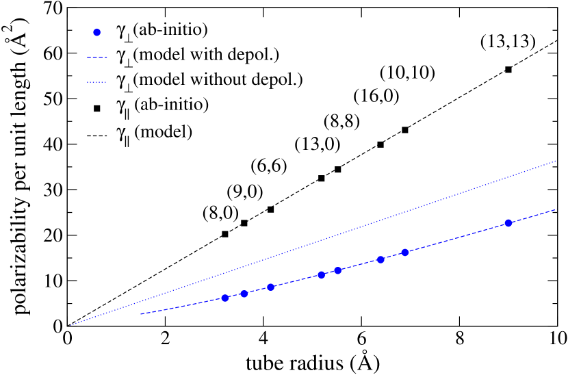
Figure 2: Perpendicular ($\gamma_{\perp}$) and longitudinal ($\gamma_{\parallel}$) polarizabilities per unit length of different BN-nanotubes: ab-initio and our generalized bond polarizability model. The influence of depolarization can be seen for $\gamma_{\perp}$.

As a first application of the generalized bond-polarizability model, we present in Fig. 2 the polarizability $\gamma$ (per unit length) of different BNNTs claus2dim . For the polarizability along the tube axis (z-direction), the model (Eq. (5)) agrees almost perfectly with our ab-initio calculations. The polarizability is proportional to the number of bonds in the unit-cell which is proportional to the tube radius. For the perpendicular direction, the model calculations overestimate the ab-initio values considerably. This discrepancy demonstrates the importance of depolarization effects in the perpendicular direction: due to the inhomogeneity of the charge distribution in this direction, an external field induces local fields which counteract the external field and thereby reduce the overall polarizability. The size of this effect can be estimated from a simple model. Imagine a dielectric hollow cylinder of radius $R$ (measured at the mid-point between inner and outer wall) and thickness $d$. The dielectric constant in tangential direction, $\epsilon_{\parallel}=(d+4\pi\beta_{\parallel})/d$, is different from the dielectric constant in radial direction, $\epsilon_{\perp}=d/(d-4\pi\beta_{\perp})$. Here, $\beta_{\parallel}$ and $\beta_{\perp}$ are the polarizabilities per unit area of the BN-sheet which are extracted from the bulk calculation claus1dim . The polarizability $\gamma$ per unit length of the cylinder due to an external homogeneous electric field perpendicular to the tube axis is henr96

$$\gamma(R)=-\frac{1}{2}\left(R+\frac{d}{2}\right)^{2}\frac{(\epsilon_{\parallel}\epsilon_{\perp}-1)(1-\Theta^{2\nu})}{(\sqrt{\epsilon_{\parallel}\epsilon_{\perp}}-1)^{2}\Theta^{2\nu}-(\sqrt{\epsilon_{\parallel}\epsilon_{\perp}}+1)^{2}},$$ (7)

with $\Theta=(R-d/2)/(R+d/2)$ and $\nu=\sqrt{\epsilon_{\parallel}/\epsilon_{\perp}}$. In the limit $R/d\rightarrow\infty$, the polarizability in Eq. (7) displays a linear dependence on the radius: $\gamma(R)\rightarrow\gamma_{0}(R)-\delta$, where $\gamma_{0}(R)=\pi(\beta_{\parallel}+\beta_{\perp})R$. This corresponds to the polarizability without depolarization effects and coincides with the undamped model curve for $\gamma_{\perp}$ (dotted line in Fig. 2).

The depolarization effects are introduced into our model by multiplying the undamped model curve for the perpendicular polarizability with the “damping” factor $\Gamma(R)=\gamma(R)/\gamma_{0}(R)$. This factor depends on the cylinder thickness $d$. The value $d=3$Å, which corresponds approximately to the full width of the charge-density of a BN-sheet, leads to an almost perfect agreement between model and ab-initio calculations.footd

To compute Raman intensities we make the further assumption:

$$B_{ij}^{k\gamma}=\frac{\partial(\Gamma_{ij}\alpha_{ij})}{\partial u_{k\gamma}}\simeq\Gamma_{ij}\frac{\partial\alpha_{ij}}{\partial u_{k\gamma}},$$ (8)

where $\partial\alpha_{ij}/\partial u_{k\gamma}$ is constructed according to Eq. 6. We assume here that to first order the atomic displacement does not change the depolarization. For $i=j=3$, i.e., for incoming and scattered light polarized along the tube axis, $\Gamma_{ij}=1$, otherwise $\Gamma_{ij}=\Gamma(R)$.

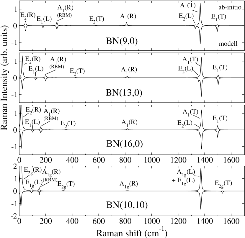
Figure 3: Raman spectrum for different BN tubes: Comparison of ab-initio calculations (positive axis) with the bond-polarization model (inverted axis). Symmetry assignment follows Ref. dam01, . The letters R,T,L denote the character of the corresponding phonon oscillation: radial, transverse, or longitudinal (see Ref. wir03, ).

In Fig. 3 we present the ab-initio and model Raman spectra for the (9,0), (13,0), and (16,0) zigzag BN nanotubes and a (10,10) armchair tube. The latter two have diameters (12.8 Åand 13.8 Å) in the range of experimentally produced BN tubes cho95 ; lee01 . The spectra are averaged over the polarization of the incoming light and scattered light. We first discuss the spectra of the zigzag tubes. The peaks below 700 cm^-1 are due to low frequency phonon modes which are derived from the acoustic modes of the sheet and whose frequencies scale inversely proportional to the tube diameter (except for the E₂(R) mode which scales with the inverse square of the diameter) wir03 . The E${}_{2}(R)$ mode gets quite intense with increasing tube diameter, but its frequency is so low that it will be hard to distinguish it from the strong Raleigh-scattering peak in experiments. The E₁(L) peak has almost vanishing intensity in the ab-initio spectrum and is overestimated in the model. The radial breathing mode (RBM) yields a clear peak which should be easily detectable in Raman measurements of BNNTs just as in the case of CNTs. Both ab-initio and model calculations yield a similar intensity for this peak. The high-frequency modes above 700 cm^-1 are derived from the optical modes of the sheet and change weakly with diameter. The A₁(R) mode at 810 cm^-1 gives a small contribution which might be detectable. The intensity decreases, however, with increasing diameter. The model only yields a vanishingly small intensity for this peak. At 1370 cm^-1 a clear signal is given by the A₁(T) mode which has very similar intensity both in model and ab-initio calculations. The small side peak at slightly lower frequency is due to the E₂(L) mode. The E₁(T) peak at 1480 cm^-1 is gaining intensity with increasing tube radius. The overall Raman spectrum for a (10,10) armchair tube exhibit similar trends.

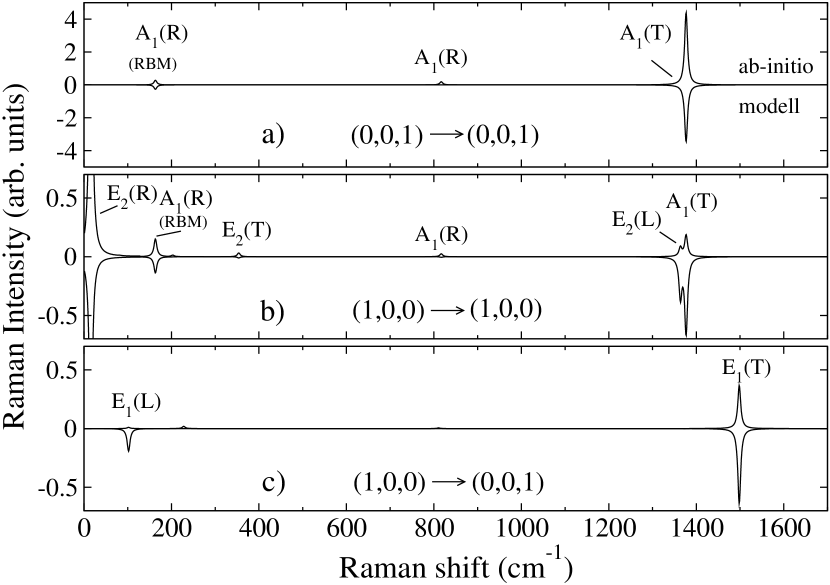
Figure 4: Raman spectrum of a BN(16,0) tube for different light polarizations ${\bf e}_{i}\rightarrow{\bf e}_{f}$. Tube oriented along (001).

In Fig. 4 we show for the (16,0) tube the dependence of the intensities on the light polarizations. If both ${\bf e}_{i}$ and ${\bf e}_{f}$ point along the tube axis (Fig. 4 a), only the A₁ modes are visible and described well by the model (except the 810 cm^-1 mode). This coincides with the finding that for the polarizability along the tube axis, depolarization does not play a role mar03 . The E modes are only visible if at least one of ${\bf e}_{i}$ and ${\bf e}_{f}$ has a component perpendicular to the tube axis (Fig. 4 b and c). The bond polarizability model reproduces these peaks, but tends to overestimate the E modes. The inclusion of depolarization effects is absolutely mandatory. Without depolarization, the model overestimates the Raman intensities for perpendicular polarization by about a factor of 15. Other discrepancies are due to the assumption in Eq. (8).

In conclusion, we implemented the bond polarizability model for BN nanotubes with parameters taken from ab-initio calculations and under inclusion of depolarization effects. Going beyond previous models for graphitic systems, our calculations yield different parameters for the in-plane and out-of-plane perpendicular polarizabilities. Good agreement between model and ab-initio calculations of the non-resonant Raman spectra of BN nanotubes is obtained for light polarization along the tube axis. For perpendicular polarization, the inclusion of depolarization effects leads to a reasonable agreement between model and ab-initio spectra. The model is implemented for single-wall BN tubes but can be extended to multi-wall tubes if the strength of the depolarization effects is modeled accordingly. A similar bond-polarizability model can also be developed for the non-resonant Raman spectra of semiconducting carbon NTs. However, due to the metallic behavior, a bond-polarizability model is not applicable to the graphene sheet. Consequently, the modeling of the polarizability of semiconducting tubes is very sensitive to the band-structure benedict , in particular to the band-gap which depends on the radius and chirality of the tubes. This work was supported by EU Network of Excellence NANOQUANTA (NMP4-CT-2004-500198) and Spanish-MCyT. Calculations were performed at IDRIS and CEPBA supercomputer centers.

References

- (1) Light Scattering in Solids II, edited by M. Cardona and G. Güntherodth (Springer-Verlag, Berlin, 1982).
- (2) A. M. Rao et al., Science 275, 187 (1997).
- (3) A. M. Rao et al., Phys. Rev. Lett. 84, 1820 (2000).
- (4) G. S. Duesberg et al, Phys. Rev. Lett. 85, 5436 (2000).
- (5) R. Saito et al., Phys. Rev. B 57, 4145 (1998).
- (6) R. Saito, G. Dresselhaus, and M. S. Dresselhaus, Physical Properties of Carbon Nanotubes (Imperial College Press, London, 1998).
- (7) A. Rubio, J. L. Corkill, and M. L. Cohen, Phys. Rev. B 49, R5081 (1994); X. Blase, A. Rubio, S. G. Louie, and M. L. Cohen, Europhys. Lett 28, 335 (1994).
- (8) N. G. Chopra et al., Science 269, 966 (1995).
- (9) R. S. Lee et al., Phys. Rev. B 64, 121405(R) (2001).
- (10) L. Wirtz, A. Rubio, R. Arenal de la Concha, and A. Loiseau, Phys. Rev. B 68, 045425 (2003); L. Wirtz and A. Rubio, IEEE Trans. Nanotech. 2, 341 (2003).
- (11) D. Sánchez-Portal and E. Hernández, Phys. Rev. B 66, 235415 (2002).
- (12) V. N. Popov, Phys. Rev. B 67, 085408 (2003).
- (13) S. Baroni, S. de Gironcoli, A. Dal Corso, and P. Giannozzi, Rev. Mod. Phys. 73, 515 (2001).
- (14) X. Gonze et al., Comp. Mat. Sci. 25, 478 (2002).
- (15) M. Lazzeri and F. Mauri, Phys. Rev. Lett. 90, 036401 (2003).
- (16) M. V. Wolkenstein, C. R. Acad. Sci. URSS 30, 791 (1941).
- (17) P. Umari, A. Pasquarello, and A. Dal Corso, Phys. Rev. B 63, 094305 (2001).
- (18) We use a periodic supercell with an intersheet distance of 12 a.u. We use Troullier-Martins pseudopotentials. The two dimensional Brillouin zone is sampled by a 1212 Monckhorst-Pack grid. Local density approximation is used.
- (19) The polarizability perpendicular to the sheet is calculated through the 1-dimensional Clausius-Mossotti relation while the parallel polarizability obeys the relation . is the unit-cell volume. We checked numerically that the thus obtained and are independent of the inter-sheet distance. The polarizability per unit area, , is , where is the unit-cell area in the x-y-plane.
- (20) The perpendicular tube polarizability is extracted from the bulk dielectric tensor through the 2-dimensional Clausius-Mossotti relation . We checked numerically that the calculated is approximately independent of the inter-tube distance.
- (21) L. Henrard and Ph. Lambin, J. Phys. B: At. Mol. Opt. Phys. 29, 5127 (1996).
- (22) The dependence on the empirical parameter is weak: For the (16,0) tube, changing from 2.2 Åto 4 Ågives rise to a change of 2 % in the perpendicular polarizability.
- (23) O. E. Alon, Phys. Rev. B 64, 153408 (2001).
- (24) A. G. Marinopoulos, L. Wirtz, A. Marini, V. Olevano, A. Rubio, and L. Reining, Appl. Phys. A 78, 1157 (2004);
- (25) L. X. Benedict, S. G. Louie, and M. L. Cohen, Phys. Rev. B 52, 8541 (1995).