Inversion phenomenon and phase diagram of the $S=1/2$ distorted diamond chain with the $XXZ$ interaction anisotropy

Abstract

We discuss the anisotropies of the Hamiltonian and the wave-function in an $S=1/2$ distorted diamond chain. The ground-state phase diagram of this model is investigated using the degenerate perturbation theory up to the first order and the level spectroscopy analysis of the numerical diagonalization data. In some regions of the obtained phase diagram, the anisotropy of the Hamiltonian and that of the wave-function are inverted, which we call inversion phenomenon; the Néel phase appears for the $XY$-like anisotropy and the spin-fluid phase appears for the Ising-like anisotropy. Three key words are important for this nature, which are frustration, the trimer nature, and the $XXZ$ anisotropy.

1 Introduction

In quantum spin chains, a value of the anisotropy of the $XXZ$ type interaction is an important factor regarding to what kind of the ground state is realized. In a case of an $S=1/2$ $XXZ$ chain, for instance, the Ising-like anisotropy brings about the Néel or ferromagnetic ground state, and the $XY$-like anisotropy brings about the spin-fluid (SF) ground state (see Fig.1(a)). In a case of an $S=1$ $XXZ$ chain, the Ising-like anisotropy also brings about the Néel or ferromagnetic ground state (see Fig.1(b)). However, this relation between the anisotropy and the ground state is sometimes broken for frustrated systems. In fact, a novel nature in the ground-state phase diagram has been found by Okamoto and Ichikawa[1]. That is, this relation is inverted in an $S=1/2$ distorted diamond (DD) chain[3, 4, 5] with the $XXZ$ type interaction. Namely, the SF state appears for the Ising-like anisotropy in some regions of the phase diagram of the ground state, and the Néel state appears for the $XY$-like anisotropy (see Fig.1(c)). This inversion between the anisotropy of the Hamiltonian and that of the wave-function in the ground state is called the inversion phenomenon. From the viewpoint of the quantum statistical physics, this phenomenon is novel and exotic. It is found by one of the present authors (K.O.) that the inversion phenomenon also appears in an $S=1/2$ trimerized $XXZ$ chain with the next-nearest-neighbor interaction.[2]

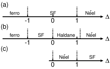
Figure 1: Schematic diagrams of the relation between the ground state and anisotropy for (a) a simple $S=1/2$ $XXZ$ chain, (b) a simple $S=1$ $XXZ$ chain, and (c) a DD chain for certain parameter sets. Here, $\Delta$ denotes the anisotropy (see Eq.(2)), and ferro, SF, and Haldane denote the ferromagnetic state, the spin-fluid state, and Haldane state, respectively.

In this paper, we elucidate the origin of the inversion phenomenon. We discuss the generalized DD chain model with the three kinds of the anisotropy parameters sketched in Fig.2. The Hamiltonian is

$${\cal H} = J_{1}\sum_{j}\{{\mib S}_{3j-1}\cdot{\mib S}_{3j}(\Delta_{1})+{\mib S}_{3j}\cdot{\mib S}_{3j+1}(\Delta_{1})\}$$ (1)

$$+J_{2}\sum_{j}{\mib S}_{3j+1}\cdot{\mib S}_{3j+2}(\Delta_{2})$$

$$+J_{3}\sum_{j}{\mib S}_{3j}\cdot{\mib S}_{3j+2}(\Delta_{3}),$$

where

$${\mib S}_{i}\cdot{\mib S}_{j}(\Delta)\equiv S_{i}^{x}S_{j}^{x}+S_{i}^{y}S_{j}^{y}+\Delta S_{i}^{z}S_{j}^{z},\quad\Delta>0,$$ (2)

and $J_{1}$ denotes the intra-trimer coupling, and $J_{2}$ and $J_{3}$ the inter-trimer couplings. All the couplings are supposed to be antiferromagnetic ($J_{1}$,$J_{2}$,$J_{3}>0$). Okamoto and Ichikawa[1] discussed the case of $\Delta_{1}=\Delta_{2}=\Delta_{3}$. We use the generalized version to investigate the relation between the anisotropy parameter and the inversion phenomenon. Hereafter we consider a case, where $J_{1}\gg J_{2},J_{3}$.

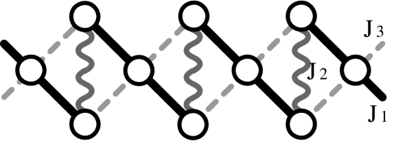
Figure 2: A sketch of the DD chain: solid lines, wavy lines, and dotted lines denote $J_{1}$, $J_{2}$, and $J_{3}$ coupling bond, respectively.

2 Phase diagram

Let us discuss the ground state of the Hamiltonian Eq.(1) using the degenerate perturbation theory[6, 7, 4] (DPT) up to the first order. First, we consider a $J_{2}=J_{3}=0$ case which is merely a three-spin problem. The ground states of the $j$-th trimer are

$$|\Uparrow_{j}\rangle \equiv\frac{1}{\sqrt{2+\lambda^{2}}}\left(|\uparrow\uparrow\downarrow\rangle-\lambda|\uparrow\downarrow\uparrow\rangle+|\downarrow\uparrow\uparrow\rangle\right)(S_{\rm tot}^{z}=1/2),$$ (3)

$$|\Downarrow_{j}\rangle \equiv\frac{1}{\sqrt{2+\lambda^{2}}}\left(|\uparrow\downarrow\downarrow\rangle-\lambda|\downarrow\uparrow\downarrow\rangle+|\downarrow\downarrow\uparrow\rangle\right)(S_{\rm tot}^{z}=-1/2),$$ (4)

where $|\uparrow\uparrow\downarrow\rangle$ denotes $|\uparrow\rangle_{3j-1}\otimes|\uparrow\rangle_{3j}\otimes|\downarrow\rangle_{3j+1}$, and $\lambda$ is a constant

$$\lambda=\frac{\Delta_{1}+\sqrt{\Delta_{1}^{2}+8}}{2}>\sqrt{2}\quad(\Delta_{1}>0).$$ (5)

Expectation values of the $z$-component of the spin are

$$\langle\Uparrow_{j}|S_{3j\pm 1}^{z}|\Uparrow_{j}\rangle=-\langle\Downarrow_{j}|S_{3j\pm 1}^{z}|\Downarrow_{j}\rangle=\frac{\lambda^{2}}{2(\lambda^{2}+2)}>0,$$ (6)

$$\langle\Uparrow_{j}|S_{3j}^{z}|\Uparrow_{j}\rangle=-\langle\Downarrow_{j}|S_{3j}^{z}|\Downarrow_{j}\rangle=-\frac{\lambda^{2}-2}{2(\lambda^{2}+2)}<0.$$ (7)

An eigenstate of $N$-trimer system is a tensor product of an eigenstate of the $j$-th trimer Hamiltonian. Since the ground states of a trimer are doubly degenerate, the ground states $|\Psi\rangle$ of $N$-trimer system are $2^{N}$-fold degenerate and they are

$$|\Psi\rangle=\bigotimes_{j}|\psi_{j}\rangle,\quad|\psi_{j}\rangle=|\Uparrow_{j}\rangle\ \mbox{or}\ |\Downarrow_{j}\rangle.$$ (8)

Next, we consider the $J_{1}\gg J_{2},J_{3}$ case, where $J_{2}$ and $J_{3}$ terms can be treated as perturbations. As far as we consider only the first-order corrections of the perturbations, we regard $|\Psi\rangle$ as a basis of a whole Hilbert space. It is convenient to introduce the pseudo-spin operator ${\mib T}_{j}$ with $T_{j}=1/2$, by which $|\Uparrow_{j}\rangle$ and $|\Downarrow_{j}\rangle$ are expressed as $T_{j}^{z}=1/2$ and $T_{j}^{z}=-1/2$ states, respectively. The original spin operators can be represented by the pseudo-spin operators:

$$S_{3j\pm 1}^{x}\equiv-\frac{2\lambda}{2+\lambda^{2}}T_{j}^{x},\quad S_{3j\pm 1}^{y}\equiv-\frac{2\lambda}{2+\lambda^{2}}T_{j}^{y},$$ (9)

$$S_{3j\pm 1}^{z}\equiv\frac{\lambda^{2}}{2+\lambda^{2}}T_{j}^{z},$$ (10)

$$S_{3j}^{x}\equiv\frac{2}{2+\lambda^{2}}T_{j}^{x},\quad S_{3j}^{y}\equiv\frac{2}{2+\lambda^{2}}T_{j}^{y},$$ (11)

$$S_{3j}^{z}\equiv\frac{2-\lambda^{2}}{2+\lambda^{2}}T_{j}^{z},$$ (12)

within the reduced basis. By straightforward calculations, the first-order correction with respect to $J_{2}$ and $J_{3}$ can be obtained as

$${\cal H}_{\rm eff}=\sum_{j}[J_{\rm eff}^{\perp}(T_{j}^{x}T_{j+1}^{x}+T_{j}^{y}T_{j+1}^{y})+J_{\rm eff}^{z}T_{j}^{z}T_{j+1}^{z}],$$ (13)

where

$$J_{\rm eff}^{\perp} = \frac{4\lambda(\lambda J_{2}-2J_{3})}{(2+\lambda^{2})^{2}},$$ (14)

$$J_{\rm eff}^{z} = \frac{\lambda^{2}\{\lambda^{2}\Delta_{2}J_{2}-2(\lambda^{2}-2)\Delta_{3}J_{3})\}}{(2+\lambda^{2})^{2}}.$$ (15)

In Eq.(13), constant terms are omitted. This effective model is nothing but the one-dimensional spin-$1/2$ $XXZ$ model. The $XXZ$ model has three kinds of the ground states depending on the anisotropy: the ferromagnetic state, the SF state, and the Néel state. The ferromagnetic state in the ${\mib T}$-picture corresponds to the $M_{s}/3$ ferrimagnetic state in the ${\mib S}$-picture, where $M_{s}$ is the saturation magnetization. Thus, the ground state of the original system is obtained from $J_{\rm eff}^{\perp}$ and $J_{\rm eff}^{z}$ as follows.

$$\begin{array}[]{c c l}J_{\rm eff}^{z}<0\ \mbox{and}\ |J_{\rm eff}^{z}|>|J_{\rm eff}^{\perp}|&\Longrightarrow&\mbox{ferrimagnetic state}\\ |J_{\rm eff}^{z}|<|J_{\rm eff}^{\perp}|&\Longrightarrow&\mbox{spin-fluid state}\\ J_{\rm eff}^{z}>|J_{\rm eff}^{\perp}|&\Longrightarrow&\mbox{N\'{e}el state}\\ \end{array}$$

From the above inequalities, the phase diagram of the ground state with respect to three variables, $\Delta_{1}$, $\Delta_{2}$, and $\Delta_{3}$, can be obtained. The examples of the phase diagram are shown in Figs.5-8. Figures 5-5 are examples of the case in which the anisotropy parameters, $\Delta_{1}$, $\Delta_{2}$, and $\Delta_{3}$, are Ising-like. Figures 8-8 are examples of the case of the $XY$-like anisotropy parameters. Although the phase diagrams in a $\Delta_{1}\neq 1$ case are not shown in this paper, the inversion phase also appears in that case. From Figs.5-8, it is clear that the inversion phases generally appear. Only in the cases of $\Delta_{1}=1,\Delta_{2}=\Delta_{3}$, however, the inversion phases do not appear.

As a numerical check, we have also performed the numerical diagonalization using the Lanczös method and the level spectroscopy analysis.[8, 9, 10, 11] We found that the numerical results are in good agreement with the results of the perturbation theory as shown in Figs.5-8.

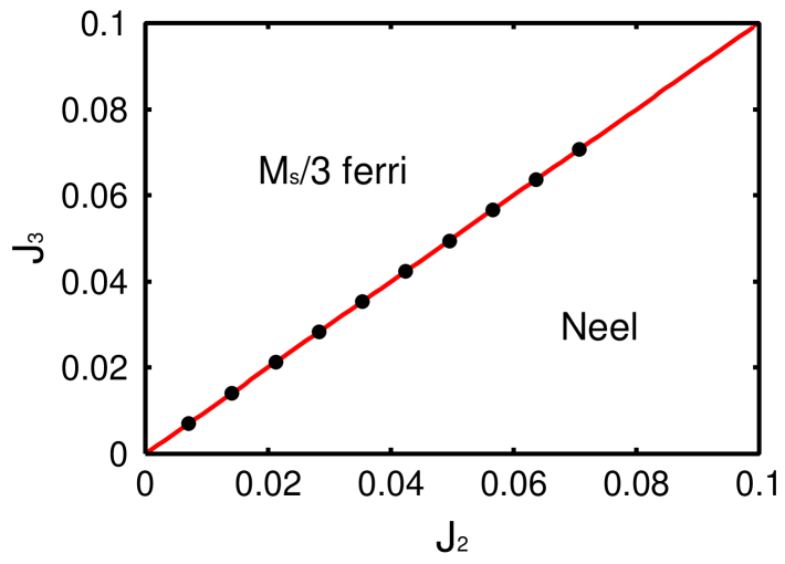
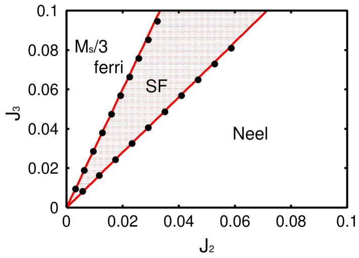
Figure 3: A phase diagram for $J_{1}=1,\Delta_{1}=1,\Delta_{2}=\Delta_{3}=2.5$. Solid line denotes the DPT result, and dots denote the numerical result.

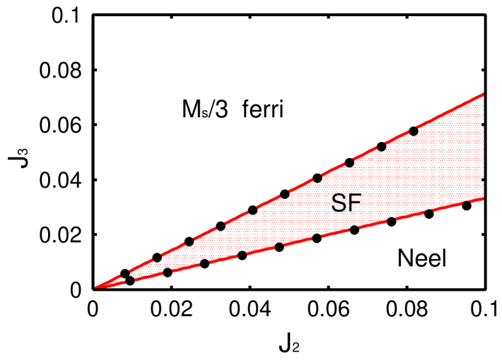
Figure 4: A phase diagram for $J_{1}=1,\Delta_{1}=1,\Delta_{2}=2.5,\Delta_{3}=1.5$. Solid lines denote the DPT result, and dots denote the numerical result.

Figure 5: A phase diagram for $J_{1}=1,\Delta_{1}=1,\Delta_{2}=1.5,\Delta_{3}=2.5$. Solid lines denote the DPT result, and dots denote the numerical result.

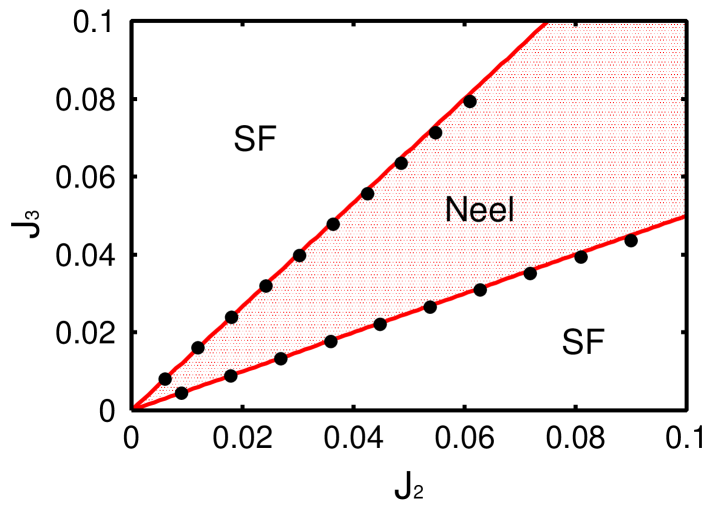
Figure 6: A phase diagram for $J_{1}=1,\Delta_{1}=1,\Delta_{2}=\Delta_{3}=0.5$.

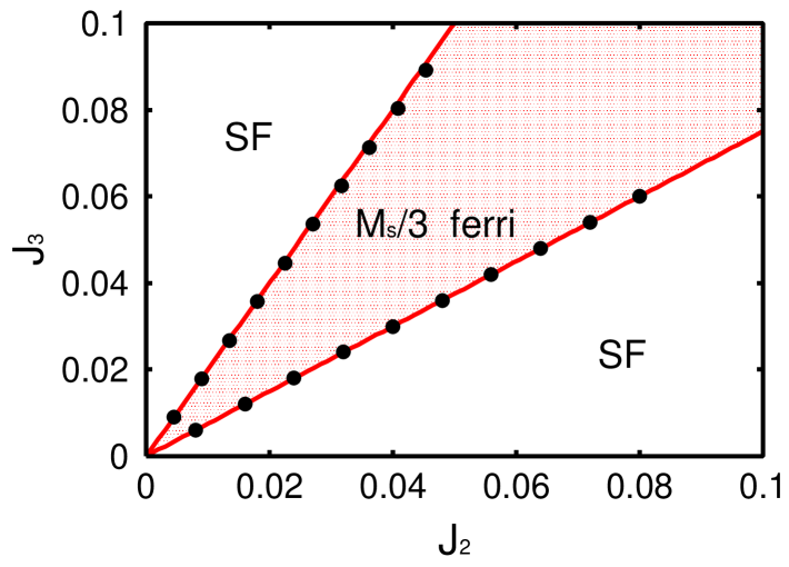
Figure 7: A phase diagram for $J_{1}=1,\Delta_{1}=1,\Delta_{2}=0.6,\Delta_{3}=0.2$. Solid lines denote the DPT result, and dots denote the numerical result.

Figure 8: A phase diagram for $J_{1}=1,\Delta_{1}=1,\Delta_{2}=0.2,\Delta_{3}=0.6$. Solid lines denote the DPT result, and dots denote the numerical result.

3 Discussion

Let us discuss the ground-state phase diagram of the DD chain qualitatively. First, we consider a case where $\Delta_{2},\Delta_{3}>1$. We note that the following discussions are qualitatively independent of $\Delta_{1}$. We discuss a correlation of neighboring trimers. Figure 9(a) shows a case where the two trimers are neighboring each other with $|\Uparrow_{j}\rangle$ and $|\Uparrow_{j+1}\rangle$.

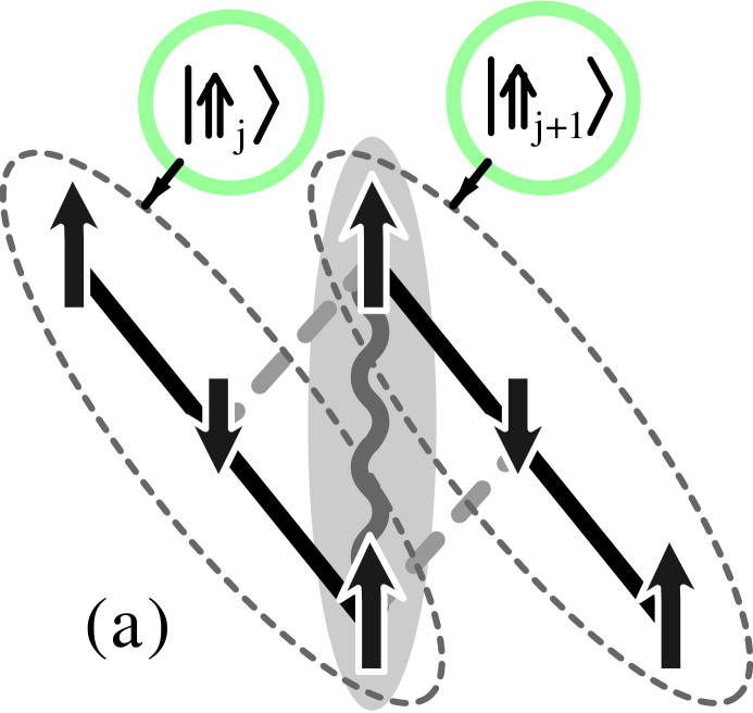
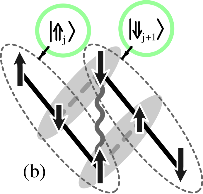
Figure 9: Schematic diagrams for the cases where two trimers are neighboring each other with (a) $|\Uparrow_{j}\rangle$ and $|\Uparrow_{j+1}\rangle$, and (b) $|\Uparrow_{j}\rangle$ and $|\Downarrow_{j+1}\rangle$. The shadow denotes a frustrated pair of spins.

Figure 9(b) shows a case where they are neighboring with $|\Uparrow_{j}\rangle$ and $|\Downarrow_{j+1}\rangle$. The couplings $J_{2}$ is frustrated for Fig.9(a) since all the interactions are antiferromagnetic. Thus, we can consider that the situation of Fig.9(a) is stable for larger $J_{3}$, while it is unstable for larger $J_{2}$. On the other hand, the coupling $J_{3}$ is frustrated for Fig.9(b). Thus, we can also consider that the situation of Fig.9(b) is stable for larger $J_{2}$, and unstable for larger $J_{3}$. Of course, we did not mention that the phase boundary is $J_{2}=J_{3}$ because its slope will depend on the values of anisotropies, as is expected from Eqs.(6)-(7). We obtain the qualitative sketch of the phase diagram shown in Fig.10(a); the area of $J_{2}<J_{3}$ is the ferrimagnetic phase and that of $J_{2}>J_{3}$ is the Néel phase.

Next, we discuss a case of $\Delta_{2},\Delta_{3}<1$. The ordering effect of the couplings $J_{2}$ and $J_{3}$ are weak, because the $\Delta_{2}$ and $\Delta_{3}$ are $XY$-like. Therefore, a whole area of the $J_{2}$-$J_{3}$ phase diagram where $J_{2},J_{3}\ll J_{1}$ will be the SF state (see Fig.10(b)).

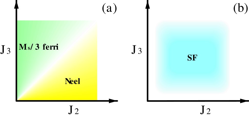
Figure 10: Schematic phase diagrams with the qualitative argument for (a)$\Delta_{2},\Delta_{3}>1$ (Ising-like) case, and (b)$\Delta_{2},\Delta_{3}<1$ ($XY$-like) case.

Comparing Fig.10 with Figs.5-8, we can see that the above discussions hit the point.

Let us proceed to the inversion phase. For Figs.5-5 and Figs.8-8, the inversion phase appears in an area $J_{1}\gg J_{2}\sim J_{3}$ where the trimer nature is still conspicuous, and $J_{2}$ and $J_{3}$ strongly compete with each other. We present an intuitive explanation in this competitive area. The interaction along the $z$-direction is stronger for the Ising-like case, by which the system is well-ordered to the Néel state in usual cases. However, the ordered state undergoes more energy loss in this area due to the competition between $J_{2}$ and $J_{3}$. Thus, the spins are going to lie in the $XY$ plane to avoid this energy loss, which brings about the disordered SF phase. A similar explanation holds for the $XY$-like case. The spins are going to lie in the $XY$-plane in usual cases, which corresponds to the SF state. In our case, since the energy loss due to the competition between $J_{2}$ and $J_{3}$ is serious, the spins are going to be pointed along the $z$-direction. Then, the ordered state (Néel or ferrimagnetic state) is realized. Another possible mechanism to avoid the energy loss due to the competing interactions is to form a singlet dimer pair. This mechanism is well known for the $S=1/2$ chain with the next-nearest-neighbor interactions.[12, 13] However, the formation of the singlet dimer pair is irreconcilable with the trimer nature. Therefore, the dimer phase does not appear for $J_{1}\gg J_{2},J_{3}$, where the trimer nature is conspicuous. In fact, we have found that the dimer phase appears in the regime $J_{1}\sim J_{2}\sim J_{3}$.[14] Thus, we have intuitively explained why the inversion phenomenon appears in this area.

Thereby, it seems that the origin of the inversion phenomenon is frustration, the trimer nature, and the $XXZ$ anisotropy. In addition, the above discussion can also predict the location of the inversion phase. The inversion phase in Fig.5 is located on the upper left side, compared to that in Fig.5. This is because of the magnitude relation between $\Delta_{2}$ and $\Delta_{3}$ as explained in the following. In the above discussion, only the couplings $J_{2}$ and $J_{3}$ are considered as the ordering effect. However, not only $J_{2}$ and $J_{3}$, but also $\Delta_{2}$ and $\Delta_{3}$ govern the orders. When $\Delta_{2}>\Delta_{3}$, the Néel state area becomes wider in Fig.5, and the inversion phase is located on the upper left side. On the other hand, the ferrimagnetic state area becomes wider in Fig.5 because $\Delta_{2}<\Delta_{3}$; this helps for the role of $J_{3}$. Comparing Figs.8-8, we can also develop a similar discussion. The inversion phase is the Néel phase in Fig.8, and it is the ferrimagnetic phase in Fig.8. When $J_{2}$ and $\Delta_{2}$ ($J_{3}$ and $\Delta_{3}$) are relatively strong in comparison with $J_{3}$ and $\Delta_{3}$ ($J_{2}$ and $\Delta_{2}$), the more stable state is Fig.10(b) (Fig.10(a)). Thus, the Néel ordering effect is stronger for Fig.8, and the ferrimagnetic phase appears for Fig.8. We can interpret that the Néel phase (the ferrimagnetic phase) is selected as the inversion phase in Fig.8 (Fig.8).

The phase diagrams of the cases of Fig.5 and Fig.8 are remarkable. The inversion phase does not appear in these phase diagrams. The result of the analytical calculation indicates that the inversion phases are always absent when $\Delta_{1}=1$ and $\Delta_{2}=\Delta_{3}$. The physical reason of the absence of the inversion phenomenon has not been understood yet.

Finally, we consider the origin of the inversion phenomenon in view of the effective model, Eqs.(13)-(15). The effective coupling constants $J_{\rm eff}^{\perp}$ and $J_{\rm eff}^{z}$ are constructed of the subtraction of the terms proportional to $J_{2}$ and $J_{3}$. Of course, the subtraction comes from the competition between couplings $J_{2}$ and $J_{3}$. It can be manifestly expected that this subtraction causes the inversion between the anisotropy of the original model and that of the effective model. For instance, we discuss the case of $\Delta_{1}=1$, where $J_{\rm eff}^{z}/J_{\rm eff}^{\perp}=(\Delta_{2}J_{2}-\Delta_{3}J_{3})/(J_{2}-J_{3})$. When $J_{2}\gg J_{3}$, we see $J_{\rm eff}^{z}/J_{\rm eff}^{\perp}\sim\Delta_{2}$ and $J_{\rm eff}^{z}>0$. Meanwhile, when $J_{2}\ll J_{3}$, it becomes $J_{\rm eff}^{z}/J_{\rm eff}^{\perp}\sim\Delta_{3}$ and $J_{\rm eff}^{z}<0$. Thus, we obtain the schematic phase diagram Fig.10. This agrees with the result of the previous qualitative discussion. On the other hand, when $J_{2}\sim J_{3}$, $J_{\rm eff}^{z}/J_{\rm eff}^{\perp}$ can be Ising-like ($XY$-like) in spite of the $XY$-like (Ising-like) $\Delta_{2}$ and $\Delta_{3}$. Here the subtraction plays a crucial role.

4 Conclusion

In this paper, we investigate the phase diagram of the ground state of the DD chain with the $XXZ$ type interaction using the degenerate perturbation theory as well as the level spectroscopy analysis of the numerical diagonalization data. The obtained phase diagrams indicate that the inversion phase is stable to various sets of anisotropies. Our discussion suggests that frustration, the trimer nature and the $XXZ$ type interaction are necessary for the inversion phenomenon. In fact, it has been found in the $S=1/2$ trimerized $XXZ$ chain with the next-nearest-neighbor interactions,[2] and also in the $S=1/2$ frustrated three-leg ladder with the $XXZ$ anisotropy. [15] Therefore, we conclude that the inversion phase may appear in the phase diagram of the ground state for models with these three key words. Unfortunately, real materials corresponding to the above models have not been found yet. However, our prediction of this interesting phenomenon may become a motivation of searching or synthesizing the corresponding materials.

5 Acknowledgments

We would like to express our appreciation to Prof. Takashi Tonegawa and Prof. Masaki Oshikawa for stimulating discussions. For the numerical diagonalization, we used the package program TITPACK ver.2 developed by Prof. Hidetoshi Nishimori, to whom we are grateful. The present work has been supported in part by a Grant-in-Aid for Scientific Research (C) (No.14540329) from the Ministry of Education, Culture, Sports, Science and Technology.

References

References

- [1] K. Okamoto and Y. Ichikawa: J. Phys. Chem. Solids 63 (2002) 1575.
- [2] K. Okamoto: Prog. Theor. Phys, Suppl. No. 145 (2002) 208.
- [3] K. Okamoto, T. Tonegawa, Y. Takahashi and M. Kaburagi: J. Phys. : Cond. Matt. 11 (1999) 10485.
- [4] A. Honecker and A. Läuchli: Phys. Rev. B 63 (2001) 174407.
- [5] K. Okamoto, T. Tonegawa and M. Kaburagi: J. Phys. : Cond. Matt. 15 (2003) 5979, and references therein.
- [6] K. Totsuka: Phys. Rev. B 57 (1998) 3435.
- [7] F. Mila: Eur. Phys. J. B 6 (1998) 201.
- [8] K. Nomura and A. Kitazawa: in Proc. French-Japanese Symp. on Quantum Properties of Low-Dimensional Antiferromagnets ed Y. Ajiro and J-P. Bouchcer (Kyushuu University Press, 2002); cond-mat/0201072.
- [9] K. Okamoto: Prog. Theor. Phys, Suppl. No. 145 (2002) 113; cond-mat/0201013.
- [10] K. Nomura and K. Okamoto: J. Phys. Soc. Jpn. 62 (1993) 1123.
- [11] K. Nomura and K. Okamoto: J. Phys. A: Math. Gen. 27 (1994) 5773.
- [12] T. Tonegawa and I. Harada: J. Phys. Soc. Jpn. 56 (1987) 2153.
- [13] K. Okamoto and K. Nomura: Phys. Lett. A 169 (1992) 433.
- [14] K. Okamoto, A. Tokuno and Y. Ichikawa: in preparation.
- [15] K. Okamoto and T. Sakai: in preparation.