Limits on the amplification of evanescent waves of left-handed materials

Abstract

We investigate the transfer function of the discretized perfect lens in finite-difference time-domain (FDTD) and transfer matrix (TMM) simulations; the latter allow to eliminate the problems associated with the explicit time dependence in FDTD simulations. We argue that the peak observed in the FDTD transfer function near the maximum parallel momentum $k_{\|,\mathrm{max}}$ is due to finite time artifacts. We also find the finite discretization mesh acts like imaginary deviations from $\mu=\varepsilon=-1$ and leads to a cross-over in the transfer function from constance to exponential decay around $k_{\|,\mathrm{max}}$ limiting the attainable super-resolution. We propose a simple qualitative model to describe the impact of the discretization. $k_{\|,\mathrm{max}}$ is found to depend logarithmically on the mesh constant in qualitative agreement with the TMM simulations.

The ability of the left-handed finite slab with a homogeneous permeability $\mu=-1$ and permittivity $\varepsilon=-1$ to form a perfect lens (PL) has received much attention since first proposed by PendryPendry00 . Such a slab does not only compensate the phase of the propagating waves emanating from a point source to form a focus on the opposite side of the slab. It also amplifies the evanescent waves which decay exponentially in vacuum into exponentially growing solutions inside the slab. This way all the source amplitudes reemerge in the focus. The immediate consequence of this behavior is that the resolution of the image may overcome the diffraction limit. Soon after, it was realizedRamakrishna02 ; Smith03 that the restoration of the evanescent waves by the PL is exceptionally sensitive to small deviations from $\mu=\varepsilon=-1$. The transfer function of the PL, defined by the amplitude ratio of a plane wave component at the focus and the source, is, in the ideal case, unity for all $\omega$ and $k_{\|}$ up to infinity. For the near-perfect lens it exposes an order of unity ($o(1)$) behavior at small parallel momenta $k_{\|}$ which turns into exponential decay $\sim e^{-k_{\|}d}$ for large $k_{\|}$. The cross-over between $o(1)$ behavior and exponential decay for a given PL defines a maximum parallel momentum $k_{\|,\mathrm{max}}$ which qualitatively constitutes the highest evanescent wave still restored by the PL, hence, defines the maximum attainable sub-wavelength resolution $\Delta x_{\mathrm{min}}\sim 2\pi/k_{\|,\mathrm{max}}$. For small deviations $\mu=\varepsilon=-1+\gamma$ with $\gamma\in{\bf C},\ |\gamma|\ll 1$ from the ideal PL a logarithmic dependence $k_{\|,\mathrm{max}}\,d\sim-\log\,|\gamma|$ of the cross-over momentum has been foundSmith03 . Here and throughout the paper we employ a dimensionless formulation measuring all lengths in units of the linear size $L$ of the unit cell and all frequencies in units of the vacuum speed of light divided by $L$. In particular, this renders the dimensionless vacuum speed of light $c=1$ and wavelength $\lambda=2\pi/\omega$.

Almost all numerical investigations of the PL’s imaging properties deploy finite-difference time domain (FDTD) simulation using a time and space discretized version of the Maxwell equations. After a few contradictory publicationsZiolkowski01 ; Fang03 ; Cummer03 , Rao and OngRao03a ; Rao03b established the amplification of the evanescent waves inside the LH material slab and the cross-over behavior in the transfer function numerically for the FDTD method. They also observed the occurrence of surface plasmons, ie. local field enhancement, at the first interface for the slightly lossy PL. The FDTD simulations of the PL suffer from explicit time dependence. Since the time domain simulations involve a finite time window from the "switch-on" to the actual measurement of the fields, the results are obtained as a superposition of a finite width $\omega$-distribution around the target frequency $\omega_{0}$ which narrows as the simulation time increases. The corresponding transfer function $t_{\mathrm{FDTD}}(\omega_{0})$ differs considerably from the stationary (frequency-domain for a single frequency $\omega$) transfer function $t_{\infty}(\omega)$. In conjunction with the physically always present dispersion $\mu(\omega)$, $\varepsilon(\omega)$ of the left-handed material this leads to a possible coupling to the surface plasmons on both interfaces of the slab which in turn causes convergence problems in the FDTD. The FDTD only converges for the near-perfect lens where the surface plasmons are damped by the small imaginary part in the LH slabRao03b ; GomezSantos03 . If we approach the ideal PL the FDTD ceases to converge which renders the method unusable.

Due to the existence of surface plasmons at the LH slab the transfer function of the near-perfect lens includes poles along the surface plasmon dispersion relationGomezSantos03 which can be approximated by $-\tanh(k_{\|}d/2)=-1\pm\gamma$ for $k_{\|}$ well above the propagating modes. By virtue of the LH materials dispersion relation this essentially real $\gamma$ directly translates into a frequency deviation from $\omega_{0}$. The poles approach $\omega_{0}$ exponentially for growing $k_{\|}$. For small $k_{\|}$ the poles of the surface plasmons are usually outside the finite width $\omega$-distribution, we find convergence of the FDTD and the transfer function is dominated by the stationary transfer function $t_{\infty}(\omega)$ at $\omega_{0}$. For large $k_{\|}$ the poles are exponentially damped in all lossy cases and cease to contribute either. However, for intermediate $k_{\|}\approx k_{\|,\mathrm{max}}$ the surface plasmon poles constitute the principal contribution to $t_{\mathrm{FDTD}}(\omega_{0})$. This leads to non-convergence of the FDTD due to the emerging "beating pattern", modulated by the frequency difference of the two surface plasmon branches as explained by Gómez-SantosGomezSantos03 . As we emphasize here, this also explains the unexpected peak $t_{\mathrm{FDTD}}(\omega_{0})\gg 1$ around $k_{\|,\mathrm{max}}$ in the FDTD transfer function found by Rao and OngRao03a and also confirmed by our own FDTD simulations. The peak originates from the contribution of the diverging $t_{\infty}(\omega_{\mathrm{pole}})$ to the magnitude of $t_{\mathrm{FDTD}}(\omega_{0})$. Analytically we would expect a monotonous transition from the $o(1)$ behavior below the cross-over momentum below $k_{\|,\mathrm{max}}$ to exponential decay above for the near-perfect lens.

In general we are interested in the stationary case transfer function $t_{\infty}(k_{\|},\omega,d)$ of the PL as this allows us to estimate the imaging properties. The field components in the focus are given by the field components in the source as

$$E_{\mathrm{focus}}(k_{\|},t)\ =\ \int d\omega\ t_{\infty}(k_{\|},\omega)\,E_{\mathrm{source}}(k_{\|})\,g(\omega,\omega_{0})\,e^{i\omega t}$$

where $g(\omega,\omega_{0})$ is the frequency distribution around the frequency of the point source due to the switch-on of the source and the finite observation time window. $E_{\mathrm{source}}(k_{\|})$ and $g(\omega,\omega_{0})$ are parameters of the setup and measurement, only $t_{\infty}(k_{\|},\omega)$ is an intrinsic property of the lens. In the FDTD this stationary transfer function $t_{\infty}(k_{\|},\omega)$ is only accessible via the temporal Fourier transform of the simulation results which is neither convenient nor especially robust against numerical error.

In contrast, the transfer matrix method (TMM) simulations provide a means to directly obtain the stationary transfer function for a single frequency. We can simulate transmission and reflection amplitudes as well as the spatial field distribution without the artifacts of finite time simulations. In order to eliminate the effect of numerical error we employ an arbitrary-precision implementation of the TMM described for instance in Ref. Markos02a, .

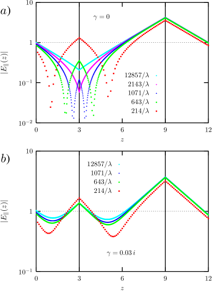
Figure 1: (Color online) The distribution of the electric field in TE mode is shown from source ($z=0$) to focus ($z=12$) across the lossless (a) and lossy (b) perfect lens for successively finer discretization. The left-handed slab between the interfaces at $z=3$ and $z=9$ has $\mu=\varepsilon=-1$ for the lossless PL and $\mu=\varepsilon=-1+\gamma$ with $\gamma=0.03\,i$ for the lossy PL. We discretized using a uniform cubic mesh with a linear resolution ranging from 240 to 12857 mesh points per vacuum-wavelength.

Fig. 1(a) shows the TMM simulated spatial field distribution for the parallel component of the E field in TE polarization across a PL for one particular evanescent wave component with $k_{\|}=1.89\,\omega$ and several spatial discretizations ranging from 240 to 12857 linear mesh points per vacuum-wavelength. The LH slab extends from $z=3$ to $z=9$, which corresponds to a thickness of $0.28\lambda$. The vertical solid lines indicate the interfaces. The source is located at $z=0$ and we get an image at $z=12$. Note that despite the elimination of the explicit time-dependence of the FDTD simulations we still observe unexpected field enhancement at the first interface of the PL. These artifacts are easily associated with the finite discretization leading to reflection of incident evanescent modes at the first interface. Only for very fine discretization meshes the field distribution approaches the analytically expected zig-zag-form featuring a minimum at the first interface. For coarse discretizations we observe a prominent maximum at the first interface accompanied by (almost) zeros of the fields before and after the interface indicating a phase shift of the response of the interface. In Fig. 1(b) we show the corresponding field distributions for the lossy PL where a small imaginary part $\gamma=0.03\,i$ is added to the permeability and permittivity of the LH slab. Again we observe the field enhancement at the first interface, but the zeros of the field have disappeared. However, in this case the behavior is dominated by the losses in the LH slab and the dependence on the discretization is much weaker. The observed dependence on the imaginary part for fixed discretization (not shown) confirms previous results obtained from FDTD simulationsRao03a .

For the lossy PL there is a simple physical explanation for the reflection of evanescent waves and the occurrence of surface modes at the first interface: For the evanescent waves in vacuum between source and first interface ${k}_{\|}$ is real and ${k}_{\bot}$ purely imaginary. Whenever the PL involves an (causal) imaginary part or the evanescent solutions on the right hand side of the slab couple to propagating modes or are subject to absorption, electromagnetic field energy is dissipated in the system. This energy has to be provided by the source and transmitted across the vacuum gap before the PL. Although it is well known that a single evanescent wave cannot transmit energy this is not true for a superposition $A\,e^{i({\bf k}_{\|}+{\bf k}_{\bot}){\bf r}}+B\,e^{i({\bf k}_{\|}-{\bf k}_{\bot}){\bf r}}$ of incoming and reflected evanescent wave component. The general equation for the time-averaged Poynting vector for the TE mode inside the vacuum slab is

$$\left<{\bf S}\right>_{\mathrm{TE}}\ =\ \mathrm{Im}(AB^{*})\frac{i\,{\bf k}_{\bot}}{\omega\mu}\ +\$$

$$\frac{{\bf k}_{\|}}{\omega\mu}\left(\frac{|A|^{2}}{2}e^{-2\mathrm{Im}({\bf k}_{\bot}{\bf r})}+\frac{|B|^{2}}{2}e^{+2\mathrm{Im}({\bf k}_{\bot}{\bf r})}+\mathrm{Re}(AB^{*})\right)$$

and similarly for the TM mode. Considering the first term it is immediately clear that in order to have an energy current normal to the interface across the gap, $\mathrm{Im}(AB^{*})$ and thus the reflection at the first interface has to be non-zero. Note that this even applies to the ideal PL if we have an outgoing energy current or dissipation on the right hand side of the lens.

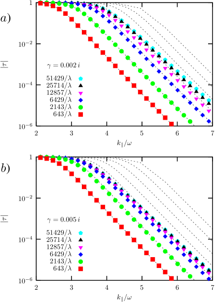
Figure 2: (Color online) The transfer function from source to focus is shown for the lossy PL (symbols) with $\mu=\varepsilon=-1+\gamma$ for two different small imaginary parts $\gamma=0.002\,i$ (a) and $\gamma=0.005\,i$ (b) and different discretizations. The dashed lines show the corresponding transfer function for the lossless PL. We discretized using a uniform cubic mesh with a linear resolution ranging from 643 to 51429 mesh points per vacuum-wavelength. The additional rightmost dashed line corresponds to $102858/\lambda$.

Now we shall consider the transfer function $t_{\infty}(k_{\|},\omega,d)$ of the PL with and without losses from source to focus as obtained by the TMM. In Fig. 2 we show the dependence of the transfer function for a fixed frequency $\omega=3/10$ on the parallel momentum $k_{\|}$ for several spatial discretizations for the lossless PL and two lossy PLs with imaginary parts $\gamma=0.002\,i$ and $\gamma=0.005\,i$ added to both the permeability and the permittivity of the LH slab. Let us first consider the lossless PL represented by the dashed lines in both panels. For all discretizations there is clear evidence for a cross-over from $o(1)$ behavior to exponential decay in the $k_{\|}$ dependence of the transfer function. The cross-over occurs monotonously without a peak near $k_{\|,\mathrm{max}}$ and $k_{\|,\mathrm{max}}$ increases with finer spatial discretization. This indicates that the discretization mesh constant acts like an effective imaginary part in a continuous lossy PL. For the lossy discretized PL, ie. adding an explicit imaginary part $\gamma$ we observe the same qualitative behavior. Here the cross-over is determined by both, discretization and the losses due to the explicit imaginary parts. For small $\gamma$ and coarse discretization the behavior of the transfer function is entirely dominated by the finite discretization: the lossy PL virtually coincides with the transfer function for the lossless PL. For successively finer discretizations $\gamma$ starts to dominate the behavior, leading to a saturation of the discretization dependence of $k_{\|,\mathrm{max}}$ at a value determined by $\gamma$. These results show that for a given lossy PL there is always a minimum discretization mesh constant where the transfer function "converges", ie. becomes independent on the discretization. For the simulated lossless perfect lens the cross-over in the transfer function due to the discretization becomes the primary limiting factor for the observation of sub-wavelength resolution. In Fig. 3 we show the dependence of the cross-over momentum $k_{\|,\mathrm{max}}$ on the discretization for the lossless and two lossy $0.28\lambda$-PLs at $\omega=3/10$ as extracted from the data presented in Fig. 2. It is evident that for the lossless PL over a wide range of discretizations $k_{\|,\mathrm{max}}$ increases logarithmically with the linear number of mesh points per vacuum wavelength. For the lossy cases this slow increase saturates at a finite $k_{\|,\mathrm{max}}$ which in turn decreases with increasing deviation $\gamma$ from the lossless case. In order to achieve a moderate five-times better resolution than the one provided by the propagating modes alone for the $d=0.28\lambda$ lossless PL, we have to push the discretization to a ridiculously high value of $10^{5}$ linear mesh points per vacuum wavelength. Such discretization mesh densities are easily limited by the available computer power.

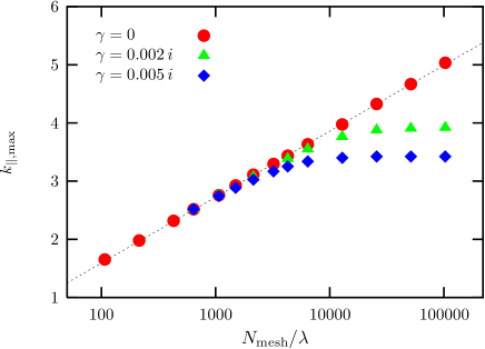
Figure 3: (Color online) The logarithmic scaling of the cross-over parallel momentum $k_{\|,\mathrm{max}}$ with the number of linear mesh points per vacuum-wavelength is shown for the lossless ($\gamma=0$) and two lossy PLs with $\gamma=0.002\,i$ and $\gamma=0.005\,i$. The dotted line is a fit $k_{\|,\mathrm{max}}d=(24/27)\log\,(4\lambda/N_{\mathrm{mesh}})$ for the lossless PL.

The effect of the discretization can be qualitatively understood in terms of a simple model. In the standard discretization of the Maxwell equations the E and H field components are assigned to the links of two mutually dual latticesTavlove . As a consequence a wave traveling towards the surface of a discretized homogeneous slab will first "see" the electric response and approximately half a mesh step later the magnetic response (or vice versa, depending on the material discretization and definition of the interface). This can be analytically modeled assuming a continuum lossless PL with $\mu=\varepsilon=-1$ to be sandwiched between two thin layers with $\mu=-\varepsilon=1$ and $-\mu=\varepsilon=1$, respectively. The thickness $\delta$ of the surface layers shall be of the order of the discretization mesh constant. Now we can derive the leading order $\delta$-corrections to the transfer function analytically using the transfer matrix technique. We can calculate the total transfer matrix of the left-handed slab (${\bf\tau}_{2})$ wrapped in surface layers (${\bf\tau}_{1},{\bf\tau}_{3}$) and the two surrounding vacuum slabs (${\bf\tau}_{2})$ as

$${\bf\tau}_{\mathrm{imaging}}\ =\ {\bf\tau}_{0}(b)\,\big{[}{\bf\tau}_{3}(\delta)\ {\bf\tau}_{2}(d)\ {\bf\tau}_{1}(\delta)\big{]}\,{\bf\tau}_{0}(a).\quad$$ (2)

For the transfer matrix of an homogeneous slab in wave representation we find

$${\bf\tau}_{i}(d)\ =\ \left(\!\begin{array}[]{cc}\alpha_{i}(d)&\beta_{i}(-d)\\ \beta_{i}(d)&\alpha_{i}(-d)\end{array}\!\right)$$

with the elements

$$\alpha_{i}(d) = \cos(k_{i}d)\,+\,\frac{i}{2}\left(\zeta_{i}+\frac{1}{\zeta_{i}}\right)\sin(k_{i}d)$$ (3)

$$\beta_{i}(d) = \frac{i}{2}\left(\zeta_{i}-\frac{1}{\zeta_{i}}\right)\sin(k_{i}d).$$ (4)

The $\zeta_{i}$ are defined as $\zeta_{i}=\mu_{i}k_{0}/(\mu_{0}k_{i})$ or $\zeta_{i}=\varepsilon_{0}k_{i}/(\varepsilon_{i}k_{0})$ for the TE and TM mode, respectively; indices zero refer to quantities in vacuum. The transfer function coincides with the transmission coefficient $t$ (we choose $t_{-}$ for convenience) of the imaging scattering matrix $S_{\mathrm{imaging}}=S\big{[}\tau_{\mathrm{imaging}}\big{]}$,

$$t_{-}\ =\ \frac{\big{[}1+o(\delta)\big{]}\,e^{ik_{0}(a+b)}}{\cos(k_{2}d)+\Big{[}1+\delta^{2}\Big{(}\frac{2\omega^{4}}{\omega^{2}-k_{\|}^{2}}\Big{)}\Big{]}\ i\sin(k_{2}d)}.$$ (5)

We immediately recognize that the surface correction $\delta^{2}\omega^{4}/(\omega^{2}-k_{\|}^{2})=\delta^{2}\omega^{4}/k_{2}^{2}$ in the denominator acts like an imaginary part in the permeability or permittivity of the near perfect lens. If the perfect lens condition $a+b=d$ is satisfied we have $t_{-}\ =\ (1+o(\delta))/(1+\delta^{2}\omega^{4}k_{2}^{-2}(1-e^{-2ik_{2}d}))$. Let us now consider the transfer function for evanescent waves, ie. $k_{\|}>\omega$. Then $k_{2}$ is purely imaginary such that the second term in the denominator is always positive and the transfer function has no poles. If $\delta^{2}\omega^{4}k_{2}^{-2}(1-e^{-2ik_{2}d})\ll 1$, ie. for small $k_{\|}$, we can neglect the $\delta$-correction in the denominator and find an $o(1)$ behavior of the transmission function. In the opposite limit of large $k_{\|}$ we can neglect the one in the denominator and find the transfer function decaying exponentially with $k_{2}d$. The asymptotic exponential decay $t_{-}\sim k_{\|}^{2}/(\delta^{2}\omega^{4})\exp(-2k_{\|}d)$ can be used to define the cross-over momentum $k_{\mathrm{max}}\,d\ =\ -\log\,(\omega^{2}\delta/k_{\mathrm{max}})$ which has an explicit solution in terms of the product-log function,

$$k_{\mathrm{max}}\,d\ =\ -\mathrm{W}(-\omega^{2}\delta d)\ \sim\ -\log\delta$$ (6)

for small $\delta$. Since $\delta$ is assumed to be of the order of the discretization mesh constant this qualitatively represents the logarithmic dependence on the discretization observer in the TMM study above.

In conclusion we investigated the transfer function of the discretized perfect lens by means of FDTD and TMM simulations. The TMM has the advantage of computing the transfer function directly in $(k_{\|},\omega)$-space as well as eliminating the problems associated with the explicit time dependence in the FDTD simulations. We argue that the peak observed near $k_{\|,\mathrm{max}}$ in the FDTD transfer function is due to finite time artifacts; it does not exist in the TMM simulations. Further we found that the finite discretization mesh acts like an imaginary deviations from the $\mu=\varepsilon=-1$ of the PL and leads to a cross-over in the transfer function from $o(1)$ to exponential decay around a maximum parallel momentum $k_{\|,\mathrm{max}}$ limiting the attainable super-resolution of the PL. We propose a simple qualitative model to describe the impact of the discretization in terms of effective thin $\mu$-only and $\varepsilon$-only surface layers exposed by the discretized LH slab which have a thickness $\delta$ that is of the order of the discretization mesh constant. $k_{\|,\mathrm{max}}d$ is found to depend logarithmically on the mesh constant in qualitative agreement with the TMM simulations. Since virtually all simulation solve discretized Maxwell equations they are all subject to this restriction.

This work was partially supported by Ames Laboratory (Contract number W-7405-Eng-82). Financial support of EU$\underline{~{}~{}}$FET project DALHM and DARPA (Contract number MDA972-01-2-0016) are also acknowledged.

References

- (1) J. B. Pendry, Phys. Rev. Lett. 85, 3966 (2000).
- (2) S. A. Ramakrishna, J. B. Pendry D. Schurig, D. R. Smith, and S. Schultz, J. Mod. Opt. 49, 1747 (2002).
- (3) D. R. Smith, D. Schurig, M. Rosenbluth, S. Schultz, S. A. Ramakrishna, and J. B. Pendry, Appl. Phys. Lett. 82, 1506 (2003).
- (4) R. W. Ziolkowski and E. Heyman, Phys. Rev. E 64, 056625 (2001).
- (5) N. Fang and X. Zhang, Appl. Phys. Lett. 82, 161 (2003).
- (6) S. A. Cummer, Appl. Phys. Lett. 82, 1503 (2003).
- (7) X. S. Rao and C. K. Ong, Phys. Rev. B 68, 113103 (2003).
- (8) X. S. Rao and C. K. Ong, Phys. Rev. E 68, 067601 (2003).
- (9) G. Gómez-Santos, Phys. Rev. Lett. 90, 077401 (2003).
- (10) P. Markoš and C. M. Soukoulis, Phys. Rev. E 65, 036622 (2002).
- (11) A. Taflove and S. C. Hagness, Computational Electrodynamics – The Finite Difference Time-Domain Method – 2nd ed. (ArtechHouse, Boston, 2000).