Simulation of Electron Transport through a Quantum Dot with Soft Walls

Abstract

We numerically investigate classical and quantum transport through a soft-wall cavity with mixed dynamics. Remarkable differences to hard-wall quantum dots are found which are, in part, related to the influence of the hierarchical structure of classical phase space on features of quantum scattering through the device. We find narrow isolated transmission resonances which display asymmetric Fano line shapes. The dependence of the resonance parameters on the lead mode numbers and on the properties of scattering eigenstates are analyzed. Their interpretation is aided by a remarkably close classical-quantum correspondence. We also searched for fractal conductance fluctuations. For the range of wave numbers $k_{F}$ accessible by our simulation we can rule out their existence.

I Introduction

Theoretical investigations of ballistic transport through microstructures have shown that the spectral and transport properties of phase-coherent quantum systems, commonly called ”billiards”, depend strongly on the nature of the underlying classical dynamics.Gutzwiller (1991) To date, most investigations have focused on the two limiting cases of systems with either purely chaotic or regular dynamics. However, neither of these cases is generic.Markus and Meyer (1974) For the semiconductor quantum dots that are realized in the experimentReed and Kirk (1989) a classical phase space structure with mixed regions of chaotic regular motion is expected. This is due to the fact that the boundaries of such devices are typically not hard walls (as in most theoretical investigations) but feature soft wall profiles for which such a ”mixed” phase space is characteristic.Lichtenberg and Liebermann (1992) The investigation of quantum transport through soft-walled microstructures is the primary goal of the present communication.
The mixed classical phase space results in specific transport properties. Consider, e.g., the classical escape rate from an open billiard. For a dot with “hard chaos”, i.e. a metrically transitive system, the dwell time distribution, or equivalently the length distribution $P(l)$ decays exponentially, $P(l)\sim e^{-l/\bar{l}}$ (with $\bar{l}$ being the mean path length). In a mixed system, however, trajectories can be trapped in the vicinity of regular islands, leading to an increased length distribution which typically features an algebraic decay law, $P(l)\sim(l/\bar{l})^{-\alpha}$. In those hard-wall billiards with shapes that allow for a mixed phase space, it was shown that trapped trajectories lead to quasi-bound states in the corresponding quantum transport problem and appear as isolated resonances in the conductance.Huckestein et al. (2000, 2001); Bäcker et al. (2002) In the chaotic-to-regular crossover regime also so-called “Andreev-billiards”henning ; libisch and the effect of shot noise suppressionsim02 ; aigner ; sukho have recently been discussed. Furthermore, mixed classical dynamics was proposed as a mechanism giving rise to fractal conductance fluctuations (FCF).Ketzmerick (1996) Several experiments have meanwhile been performed to test this prediction. First experimental dataSachrajda et al. (1998); Micolich et al. (2001, 2002, 2004); Crook et al. (2003) appear to support this notion. However, in the corresponding numerical studies, no fractal structure in the conductance fluctuations could be found,Huckestein et al. (2000, 2001); Bäcker et al. (2002); Takagaki and Ploog (2000) which, in part, has led to a number of theoretical works that propose alternative and sometimes even contradictory explanations for FCF.Guarneri and Terraneo (2001); Benenti et al. (2001); Budiyono and Nakamura (2003); Louis and Vergés (2000) In the present paper we inquire into the appearance of this features for transport through soft-walled quantum dots.
We calculate transport coefficients and scattering wave functions by solving the time-independent one-particle Schrödinger equation for a two-dimensional scattering device. Of particular interest is the semiclassical limit of transport, where the Fermi wavelength $\lambda_{F}=2\pi/\sqrt{2E_{F}}$ (in a.u.) is much smaller than the linear dimension $D$ of the quantum billiard, $\lambda_{F}\ll D$. This is because the ratio $(\lambda_{F}/D)$ determines the resolution with which quantum mechanics can resolve the underlying (mixed) classical phase space. Note, however, that the semiclassical limit for transport in the leads of width $d,\ \lambda_{F}\ll d$, cannot be reached. The asymptotic incoming and outgoing scattering states thus remain in the quantum regime. In the limit of large Fermi energies $E_{F}$ quantum transport simulations are quite demanding. In order to reach the high energy regime we employ the Modular Recursive Green’s Function Method (MGRM),Rotter et al. (2000, 2003) which is a variant of the standard recursive Green’s function approachAkis et al. (1997) suited for small wavelength.
For a detailed analysis of the influence of the mixed classical phase space on the quantum scattering problem we compare the classical Poincaré surface of section with the Husimi distribution derived from the scattering wavefunctions. We are thereby able to classify the isolated conductance resonances and find that a recently suggested classificationBäcker et al. (2002) in terms of scattering states corresponding to classically regular or trapped trajectories, has to be extended to include resonances which are associated with unstable periodic orbits. The quantum counterpart of these orbits (commonly called “scars”Heller (1984)) emerge in the wavefunction densities which we calculate numerically. These findings are supported by very recent experimental investigations of a soft-wall microwave billiard for which scarred wavefunction have been, indeed, observed.Kim et al. (2004) We demonstrate that the resonances in conductance follow the characteristic asymmetric Fano lineshapeFano (1961) and perform a statistical analysis of the distribution of resonance widths, amplitudes and Fano asymmetry parameters. Finally, we inquire into the occurrence of fractal conductance fluctuations.
This paper is organized as follows. In Sec. II we present the scattering device investigated in this work. Section III is dedicated to a discussion of the isolated conductance resonances and the corresponding wavefunctions. The Fano profile of the resonances is analyzed in Sec. IV. In Sec. V we discuss fractal conductance fluctuations and Sec. VI finally gives a summary of the results.

II Classical dynamics

We consider in the following a stadium-shaped quantum dot with a semicircle of radius $R$ and leads attached to the straight section (see Fig. 1a). By focusing on scattering states with odd parity under reflections $(y\rightarrow-y)$, the geometry can be reduced to one semicircle with attached leads with half of the original width. The resulting cavity boundary, including the added soft-wall potential, is depicted in Fig. 1b,c.

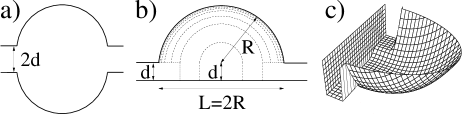
Figure 1: (a) Bunimovich stadium with leads attached at the straight segments. (b) Reduced scattering geometry consisting of a semi-circle of radius $R=1$ which is attached to a rectangle of length $L=2R$ and width $d=0.3$. The solid lines represent hard-wall boundary conditions and the dashed curves are contour lines of the soft-wall potential [for details see Eq. (3)]. (c) Illustration of the potential surface corresponding to contour plot (b).

We inject electrons from the left into this system and study the transmission and reflection probabilities classically as well as quantum mechanically. Classical simulations are performed by calculating many different trajectories of electrons with Fermi energy $E_{F}$ which enter the dot at $x=-R$. The initial positions across the lead width are uniformly distributed with an angular distribution $P(\theta)\sim\cos(\theta)$. The ballistic quantum scattering problem is solved with the Modular Recursive Green’s Function Method (MRGM).Rotter et al. (2000, 2003) We calculate scattering wave functions and the $S$ matrix of the system at different Fermi energies $E_{F}=k_{F}^{2}/2$ (in a.u.), where $N={\rm int}(d\,k_{F}/\pi)$ modes are transmitting in the leads. The total transmission $T$ is then given by

$$T=\sum^{N}_{m=1}T_{m}=\sum^{N}_{m,n=1}T_{mn}=\sum^{N}_{m,n=1}|t_{mn}|^{2}$$ (1)

with $t_{mn}$ being the transmission amplitudes from incoming mode $m$ to outgoing mode $n$. According to the Landauer formula, the conductance is obtained as

$$G=2\times T\,.$$ (2)

Atomic units ($\hbar=|e|=m_{\rm eff}=1$) will be used unless otherwise stated explicitly.
If we choose a zero potential inside the structure and hard-wall boundary conditions, the scattering device corresponds to the open Bunimovich stadium billiard which is prototypical for purely chaotic dynamics.Bunimovich (1974); Benettin and Strelcyn (1978) This behavior changes drastically if a soft wall profile is introduced (see dashed contour lines in Fig. 1b and Fig. 1c), given by:

  (3)

$$V(\vec{r}\;\!)=$$ (9)

$$\phantom{+}\ \Theta(d-y)\left\{\begin{array}[]{c@{\quad}l}-A,&|x|<0.35\\ {\rm min}[0,B(|x|\!-0.35)^{2}-A],&|x|>0.35\end{array}\right.$$

$$+\ \Theta(y-d)\left\{\begin{array}[]{c@{\quad}l}-A,&\phantom{|}S\phantom{|}<0.35\\ \phantom{\,{\rm min}[0,}B(S\phantom{|}\!-\phantom{|}0.35)^{2}-A\phantom{]}\!,&\phantom{|}S\phantom{|}>0.35\end{array}\right.\phantom{+++++}$$

with $S=|\vec{r}-\vec{d}_{0}|$ and $\vec{d}_{0}=(0,d)$. $V(r)$ rises quadratically in the exterior region of the semicircle. The potential in the rectangular region below the half-circular module depends only on the $x$-coordinate. It follows the radial profile of $V(r)$, however, only for potential values below the equipotential line of the lead such that injection and emission is barrier-free. Note that in contrast to the case where all boundaries are hard walls, the classical scattering dynamics with an arbitrary soft-wall profile is not invariant under scaling of the electron energy $E_{F}$. In order to approach the semiclassical limit of pathlength spectroscopy, we choose a scaled potential with $A=A_{0}\times E_{F}$ and $B=B_{0}\times E_{F}$. This results in classically scaling invariant dynamics and all quantum results we obtain can be compared with one and the same classical phase space structure.
As a first test of the effect the soft-wall potential has on transport, we plot in Fig. 2 the probability distribution $P(l)$ for classical trajectories to leave the cavity after a length $l$.

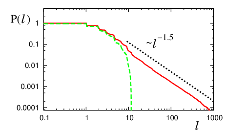
Figure 2: (Color online) Log-log plot of the classical dwell probability $P(l)$ for the cavity with soft walls (red solid line) and hard walls (green dashed line).

We find for the chaotic case with hard walls an exponential decayLin et al. (1993); Rotter et al. (2000) of $P(l)$ and for the mixed case due to the soft walls a power-law behavior which is well approximated by $P(l)\sim l^{-1.5}$ over several orders of magnitude. The difference to the chaotic case can be understood as a signature of the trapping of trajectories in the vicinity of the hierarchical set of regular islands which is typical for mixed dynamics.Meiss and Ott (1986); Ketzmerick (1996) For a more detailed phase space analysis we plot the Poincaré surface of section (PSS) of the classical dynamics in our soft-wall device. At each bounce of a trajectory against the horizontal lower boundary, the position $x$ along the boundary and the projection of the momentum vector in the horizontal direction $p_{x}$ are recorded. Fig. 3 shows the PSS for an ensemble of initial conditions with several islands of regular motion and unstable periodic orbits in an otherwise chaotic sea. Of particular interest are trajectories trapped in the vicinity of the islands (see e.g., Fig. 3i). The trapping region of phase space is shielded from the surrounding chaotic phase space by partial transport barriers which are formed by cantori as well as by stable and unstable manifolds.Lichtenberg and Liebermann (1992) A partial barrier can only be crossed through small gaps (“turnstiles”) where phase space volume is exchanged.MacKay et al. (1984) Trajectories that enter the cavity through the entrance lead first reach the chaotic part of phase space and may directly exit through the exit lead. Some trajectories do, however, cross the outermost partial barrier through a turnstile and stay trapped inside for a comparatively long time since the only path to the exit is via another or the same turnstile. Alternatively, these trajectories may get trapped even deeper inside the next layer of the hierarchical set of transport barriers. By contrast, the islands of regular motion which lie at the core of this hierarchy are invariant curves forming complete barriers and can thus not be accessed by classical trajectories emanating from the leads and contributing to transport.

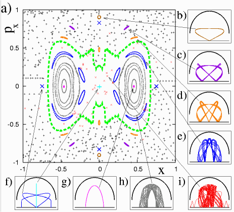
Figure 3: (Color online) Poincaré surface of section for the half-stadium with soft walls (see Fig. 1b,c). A large number of chaotic trajectories (black crosses), six regular closed orbits (b-e),(g),(h), two unstable periodic orbits (f) and one trapped chaotic trajectory (i) are shown. For orientation the arrows denote one point of the phase space representation of each trajectory. The green dashed curve shows an approximation for the outermost partial transport barrier. For details see text.

In order to determine the shape of the partial barriers and the location and size of the turnstiles the analytical methods described in Ref. MacKay et al., 1984 could, in principle, be used. It is, however, quite demanding to construct the partial barriers explicitly, in particular in the present case of soft-wall cavities where analytical solutions for trajectories are not available. We have therefore determined the outermost barrier approximately by a numerical dwell length analysis. We scan the dwell length $l$ inside the cavity on a very dense array of points in the PSS. All initial conditions which correspond to a dwell length longer (shorter) than a typical threshold value, $l_{0}=15$, are assumed to be inside (outside) the outermost partial barrier. As a result we obtain the approximate partial barrier line depicted in the PSS of Fig. 3 as a green dashed line. The location of the barrier was found to be only very weakly dependent on the choice of $l_{0}$.

III isolated resonances

Quantum dynamics profoundly modifies the phase flow in the presence of cantori in two ways: On the one hand, partial barriers become impenetrable when the phase space volume of the turnstile is smaller than that of the Planck cell $(\sim\hbar)$ i.e. the size of the minimum-uncertainty wavepacket. Consequently, phase flow is suppressed on a short time scale associated with classically allowed transitions. On the other hand, quantum mechanics opens up the possibility of barrier penetration of both complete and partial barriers by tunneling. This purely quantum transport channel is, however, in general slow and associated with the time scale for tunneling. Thus, the outermost partial barrier with turnstiles smaller than $\hbar$ divides the phase space into two distinct regions where chaotic and hierarchical eigenfunctions are concentrated on either side.Ketzmerick et al. (2000) Since the hierarchical region couples only very weakly to the leads, quasi-bound states residing in this part of phase space give rise to sharp resonances in transmission.Huckestein et al. (2000, 2001); Bäcker et al. (2002) Classically, an island of regular motion in phase space consists of a set of concentric invariant curves, each of them forming a complete barrier. Accordingly, long-lived quasi-bound states reside also in islands of regular motion and account for additional narrow resonances in transmission.
In Fig. 4 we compare the conductance (i.e. transmission) through our device as a function of the Fermi wavenumber $k_{F}$ for soft-wall and hard-wall potentials (see insets).

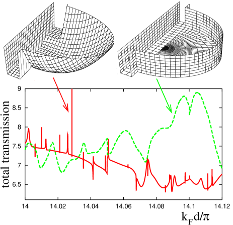
Figure 4: (Color online) Comparison between total transmission $T$ through the soft-wall (left inset) and hard-wall geometry (right inset) as a function of the Fermi wavenumber $k_{F}$ (14 lead modes are open). Narrow isolated resonances on a smoothly varying background are clearly visible for the soft wall billiard (red solid line), but are absent for the case of a hard wall boundary (green dashed line).

Note the remarkable difference between the two graphs: Sharp resonances are present in the case with a mixed phase space (see Fig. 3) and completely absent for the chaotic case. The quantum counterpart to the classical PSS is the quantum phase space distribution. In the following we analyze the Husimi distribution $H(x,p)$ at the resonance energy and investigate its localization.Bäcker et al. (2002) We define the Husimi distribution (HD) in direct analogy to the classical PSS by projection of the scattering state onto a coherent state $\phi^{\rm coherent}$ on the lower horizontal boundary.Bäcker et al. (2004) The HD reads

$$H(x,p) = |\langle\partial_{\bf n}\psi(x,y)|\phi^{\rm coherent}(x,p)\rangle|^{2}=$$

$$= \left|\int_{-1}^{1}dx^{\prime}\partial_{\bf n}\psi^{*}(x^{\prime})e^{ik_{F}p(x^{\prime}-x)-(1/2)k_{F}(x^{\prime}-x)^{2}}\right|^{2}\,,$$

where $\partial_{\bf n}\psi(x)={\bf n}(x)\cdot\nabla\psi(x,0)$ is the normal derivative of the scattering state on the lower boundary and ${\bf n}(x)$ is the vector normal to the lower cavity wall.
In Fig. 5 we show both wavefunctions and Husimi distributions for two resonant scattering states for which the quantum-classical correspondence between classical trajectories (a)-(b) and the scattering wavefunction (c)-(d) is particularly striking.

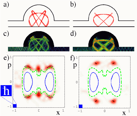
Figure 5: (Color online) (a),(b) Classical periodic orbits in the soft-wall billiards which are closely mirrored in the density $|\psi(x,y)|^{2}$ of the quantum scattering wavefunctions at the resonant energies: (c) wavenumber $k_{F}=14.0592\pi/d$ for incoming lead mode number $m=14$ and (d) $k_{F}=14.0021\pi/d,$ with $m=12$ . Figure (e) and (f) give the corresponding phase space portraits: Husimi distribution (density plot, red) and classical PSS (islands, black). For reference we also plot the outermost partial barrier (green dashed line) and the most prominent regular island (blue solid lines). The blue boxes in the lower left corner of (e),(f) indicate the size of $\hbar$ which characterizes the quantum mechanical resolution of the classical phase space.

Correspondingly, the HDs of these scattering states reside on top of the regular islands within which these periodic classical orbits propagate.
This remarkable degree of quantum-classical correspondence allows a convenient characterization of resonances in terms of the underlying phase space structure. The observed resonances fall into three classes: Resonances that are associated with the regular $(R)$ or with the hierarchical $(H)$ regions in phase space, and finally those that are associated with scars $(S)$, i.e. unstable periodic orbits in the chaotic sea. $R$ and $H$ resonances have also been found in hard-walled billiards with boundaries that allow for a mixed phase spaceBäcker et al. (2002) while scars are well-known features in bound-state wavefunctions of closed metrically transitive (“hard chaos”) systems.Heller (1984) We note that $S$ resonances have been very recently identified in soft-walled microwave billiards.Kim et al. (2004) Typical examples are shown in Fig. 6:

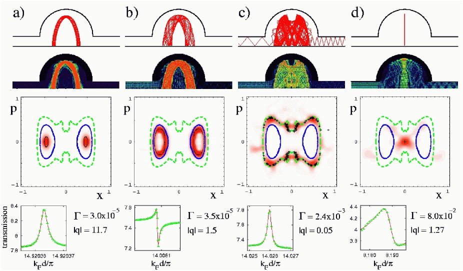
Figure 6: (Color online) Top row: Classical stable periodic orbits (a) and (b); a transiently trapped trajectory (c) and an unstable periodic orbit (d). Second row: Resonant wave function densities $|\psi(x,y)|^{2}$ closely mimicking these trajectories with wavenumbers (a) $k_{F}=14.9203\pi/d$, (b) $k_{F}=14.0061\pi/d$, (c) $k_{F}=14.0260\pi/d$, and (d) $k_{F}=8.186\pi/d$. Third row: The Husimi distributions (density plot, red) and the PSS of the corresponding trajectories (island and crosses, black). Bottom row: Transmission resonances, numerical results (green dots) and fits to the Fano resonance formula Eq. (13) (red line). Fitted values for the width $\Gamma$ and Fano asymmetry parameter $q$ are indicated.

Resonances (a) and (b) clearly fall into the class $R$, for which the HD resides on regular islands. State (a) corresponds to the center of the two prominent stable islands whereas state (b) resides near the outer border of the island. The corresponding resonance widths $\Gamma$ mirror this difference: Although both being narrow and of the same order of magnitude, $\Gamma\approx 10^{-5}$, the width decreases from the state near the outer border (b) to the state in the center of the island (a), indicating that the probability to tunnel out of the island is higher near the border than from the center of the island (for quantitative details see Fig. 6). Note that these results are in close correspondence with the findings presented in Ref. Bäcker et al., 2005.
The HD of a “hierarchical” state (c) features pronounced intensity in the region near the cantorus corresponding to a classically chaotic trajectory that gets transiently trapped inside the partial barrier. Compared to the regular states the coupling of the hierarchical states to the leads is stronger and therefore results in a resonance width $\Gamma\approx 10^{-3}$ which is typically two orders of magnitude larger than for the regular states. State (d) corresponds to a “scarred” wavefunction whose classical analogue is an unstable periodic “bouncing-ball” orbit. Its resonance width $\Gamma\approx 10^{-1}$ is even larger than of most of the hierarchical states we recorded. We note, however, that the very limited number of such scarred states which we could identify prevents us from drawing definite conclusions about the generic value of their width. Nevertheless, it is reasonable to guess that the relation found for the present system $\Gamma_{R}\ll\Gamma_{H}\ll\Gamma_{S}$ should hold in other systems as well.
The close classical-quantum correspondence in the phase structure suggests that the width of the transmission resonances can be estimated from the location of the HD relative to the cantorus. Specifically, we decompose the HD into one part that lies outside the cantorus occupying the area $A_{1}$ in the PSS and the complementary area $A_{2}$ lying inside the cantorus.
To quantify the overlap of the HD with these areas we integrate the HD according to

$$\xi_{A}=\int\!\int_{A}dx\,dp\;H(x,p)\,.$$ (11)

In Fig. 7 the ratio $\xi_{A_{1}}/(\xi_{A_{1}}+\xi_{A_{2}})$ is plotted for each resonance as a function of the resonance width $\Gamma$ for a large number of resonances which we analyzed.

Figure 7: The ratio $\xi_{A_{1}}/(\xi_{A_{1}}+\xi_{A_{2}})$ of the HDs integrated over the chaotic area $A_{1}$ outside the outermost partial barrier and over the remaining phase space area $A_{2}$ [see Eq. (11)] as a function of the resonance width $\Gamma$.

We find the proportionality

$$\Gamma\propto\left[\xi_{A_{1}}/(\xi_{A_{1}}+\xi_{A_{2}})\right]^{1.27\pm 0.12}\,.$$ (12)

Within the statistical uncertainty the deviation from linearity is most likely not significant. An approximately linear dependence on $\xi_{A_{1}}/(\xi_{A_{1}}+\xi_{A_{2}})$ could be expected for $H$ resonances and for those $R$ resonances corresponding to islands inside the cantorus. Clearly $S$ and the remaining $R$ resonances fall outside the validity of this estimate.

IV Fano profile

The isolated narrow resonances in transmission $T(k_{F})$ have typically an asymmetric Fano line shapeFano (1961) illustrated in the bottom row of Fig. 6. Fano resonances have been observed in many different fields of physics, including ballistic transport through quantum dots.Rotter et al. (2003); Nöckel and Stone (1994); Göres et al. (2000); Rotter et al. (2004a); Kobayashi et al. (2002); Rotter et al. (2004b) They occur when (at least) one resonant and one non-resonant pathway connecting the entrance with the exit channel interfere. The specific interest in analyzing Fano profiles is driven by their high sensitivity to the details of the scattering process, in particular the degree of coherence in transport and the presence of decoherent interactions with other degrees of freedom. In contrast to Breit-Wigner resonances, the asymmetric Fano resonances are not only determined by their resonance position $k_{R}$, width $\Gamma$ and amplitude $T_{0}$, but also by the Fano asymmetry parameter $q$ according to

$$T(k_{F})\approx T^{\rm offs}+T_{0}\times\frac{(k_{F}-k_{R}+q\,\Gamma/2)^{2}}{\left(k_{F}-k_{R}\right)^{2}+\left(\Gamma/2\right)^{2}}\,,$$ (13)

where $T^{\rm offs}$ is the offset value of the resonance minimum. Note that the smoothly varying background on top of which the resonance is situated is thus given by: $T^{\rm bgr}=T^{\rm offs}+T_{0}$ . The relative amplitude $A$ of the resonance (i.e. the difference between maximum and minimum value of the second term in Eq. (13)) is given byFang and Chang (1998) $A=T_{0}\times(1+q^{2})$. Due to the time-reversal symmetry in our system (i.e. no magnetic field or decoherence present) the asymmetry parameter $q$ can be treated as real and is a measure for the ratio between resonant and non-resonant transmission amplitude.Fano (1961) For $|q|\rightarrow 0$ non-resonant transmission dominates resulting in a symmetric dip at the resonant position. For $q\approx 1$ the peak is highly asymmetric. In the absence of non-resonant transmission, i.e. $|q|\rightarrow\infty$, the resonance shape approaches that of a Breit-Wigner profile. For coherent transport in the low-energy regime, where only one flux-carrying mode is open, the transmission will vary between its maximum value $T(k_{F})$ = 1 (full transmission) and $T(k_{F})=0$ near each resonance in the single-mode limit. This implies $T^{\rm offs}=0$ and $A=1$ in Eq. (13). As soon as $k_{F}$ passes the threshold $k_{F}=2\pi/d$ for opening up additional transmitting modes, Fano resonances have, in general, a minimum different from zero, $T^{\rm offs}\neq 0$.

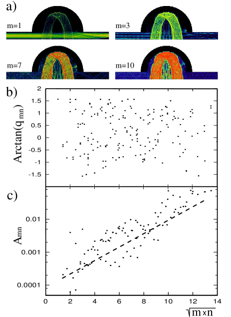
Figure 8: (Color online) (a) Wavefunction densities for selected incoming mode numbers $m$ of a typical Fano resonance [$k_{F}=14.1111\pi/d$]. For increasing $m$ the directly transmitted (non-resonant) part of the wavefunction, being dominant for $m=1$, becomes less pronounced, while the relative intensity of the $\cap$-shaped resonant part drastically increases. (b) The Fano parameter $q$ shows no correlation to the geometric mean value of the in- and outgoing mode number, $\sqrt{m\times n}$. (c) Amplitudes $A_{mn}$ are approximately proportional to $\sqrt{m\times n}$.

In order to elucidate the formation of Fano resonances we decompose the total transmission $T(k_{F})$ in terms of its contributions from different modes.Goldberger and Watson (1964) A Fano resonance observed in $T(k_{F})$ appears also as a Fano resonance in the channel transmission probabilities $T_{mn}$ at an identical position $k_{R}$ and width $\Gamma$. In general, the values for $q$ and $T_{0}$ are however different in all the $m\times n$ channels. Conversely, the sum of any number of Fano resonances with identical $\Gamma,k_{R}$ will again be a Fano resonance. Using the semiclassical connection between mode number and injection angle, $\sin\theta=m\pi/(dk_{F})$, a naive expectation would be that for the billiard geometry of Fig. 1 and low mode numbers $m,\,n$ a large fraction of transmission is mediated by direct (non-resonant) transmission and only a small part by resonant transport which corresponds to transient trapping inside the structure. Low-mode numbers in the leads correspond classically to small injection and ejection angles which, in our specific geometry, is equivalent to trajectories that connect the entrance and exit lead without exploring much of the cavity. On the other hand we expect resonant trapping to dominate for large mode numbers $m,n$. This feature is illustrated in Fig. 8a, where we plot the density of scattering wave functions with the same $k_{F}$ but different incoming mode number $m$. The resonant part of the wave function (in form of the $\cap$-shape) is strongly suppressed for the limiting case $m=1$ but increasingly pronounced for growing $m$. It is now of interestIhra (2002) to explore the dependence of the two parameters, the partial amplitude $A_{mn}$ and the Fano parameter $q_{mn}$ on the “geometric” variable $m\times n$. The lower limit $\sqrt{m\times n}=1$ corresponds to (almost) horizontal injection and ejection angles with predominant non-resonant transport (see Fig. 8a, $m=1$) whereas increasing mean values of the mode numbers stand for larger angles and therefore rising dominance of the resonant pathway. While $A_{mn}$ is approximately proportional to $m\times n$ (see Fig. 8c) indicating that with large injection and ejection angle the relative amplitude increases, we find the remarkable result that the values $q_{mn}$ are virtually uncorrelated to $m\times n$ (Fig. 8b), contrary to a naive picture. Intuitively, one would expect the asymmetry parameter $q$, being a measure for the ratio between resonant and non-resonant contributions to transmission, to systematically increase with $\sqrt{m\times n}$, but no signs of proportionality between $\sqrt{m\times n}$ and $q$ can be detected in Fig. 8b.
The projections of the resonant states onto the lead wavefunction are, however, not a basis invariant measure for transport. We therefore explore the transmission eigenvalues, i.e. the eigenvalues of the transmission operator $\hat{T}=tt^{\dagger}$ with matrix elements

$$\langle n|T|m\rangle=\sum^{M}_{k=1}\langle n|t|k\rangle\langle k|t^{\dagger}|m\rangle$$ (14)

and $n,m,k\leq M$ corresponding to the number of open modes. The transmission eigenvalues $\lambda_{i}$ ($i=1,\ldots,M$) , which we label in ascending order ($\lambda_{i}\leq\lambda_{i+1},\,\forall i=1,\ldots,M-1$), provide a channel-basis invariant representation. Implicit in this analysis is the assumption that the matrix diagonalizing $T$ is only weakly energy dependent across the width of the resonance. This is justified for narrow and non-overlapping resonances, as we have verified numerically in a few cases. We point out the similarity of this approach to the multi-channel quantum defect theory employed in atomic and molecular physics.seaton ; fritz We explore now the appearance of Fano resonances in $\lambda_{i}$ . For this purpose we determine $\lambda_{i}$ for a large number of Fano resonances and extract from each $\lambda_{i}$ the offset $T^{\rm offs}_{i}$, the amplitude $A_{i}$ and the eigenchannel Fano parameter $q_{i}$. The corresponding averages over the ensemble of Fano resonances are denoted by $\overline{T}^{\rm\,offs}_{i}$ and $\overline{A}_{i}$. As is well known from random matrix theory (RMT)Baranger and Mello (1994); Jalabert et al. (1994) the transmission eigenvalue distribution $P(\lambda)$ has the functional form $P(\lambda)=1/(\pi\sqrt{\lambda(1-\lambda)})$ , with a preponderance of eigenvalues near $\lambda=0$ and $\lambda=1$. Specific features of quantum transport are engraved in the intermediate values of the $\lambda$-distribution. As it turns out, similar conclusions apply to the properties of Fano resonances. The values for $\overline{T}^{\rm\,offs}_{i}$ , plotted as a function of the eigenchannel number $i$ in ascending order (Fig. 9) directly mirrors the $\cup$-shape of $P(\lambda)$ with a clustering of $\overline{T}^{\rm\,offs}_{i}$ in the interval $\overline{T}^{\rm\,offs}_{i}<0.1$ and $\overline{T}^{\rm\,offs}_{i}>0.9$.

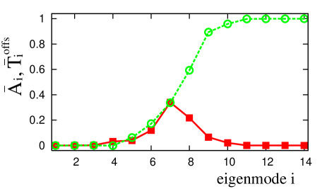
Figure 9: (Color online) Offset of transmission eigenvalues $\overline{T}^{\rm\,offs}$ (green dashed line, open circles) and amplitudes $\overline{A}_{i}$ (red solid line, squares) of the Fano resonances in the eigenmode $i$. All Fano resonances in the ensemble considered were taken from the energy interval where 14 lead modes are open, resulting in $i_{\rm max}=14$. The resonance parameters associated with the eigenmode $i$ (for ordering see text) are ensemble averaged within one specific eigenmode $i$. Note that the amplitudes $\overline{A}_{i}$ feature pronounced values only for intermediate modes $i$ where the resonance offset $\overline{T}^{\rm\,offs}$ does not take on the “classical” values close to $0$ or $1$.

Note that only a few eigenchannel numbers feature intermediate values of $\overline{T}^{\rm\,offs}_{i}$. Precisely those intermediate channels provide the dominant contribution to the resonance amplitudes $\overline{A}_{i}$ (Fig. 9). This observation suggests a simple semiclassical explanation: eigenvalues $\lambda$ close to $\lambda=0$ are associated with classical channels of “pure” reflection while those close to $\lambda=1$ are associated with “pure” transmission. Classical transmission or reflection channels correspond to classical path bundelsWirtz et al. (1997) of sufficient size in phase space ($>\hbar$, see Fig. 5), such that a quantum wavepacket can be accommodated.Silvestrov et al. (2003); jacquod Conversely, intermediate transmission values correspond to a highly structured area of phase space where the wavepacket encompasses both transmitting and reflecting classical paths giving rise to quantum indeterminism and interferences reflected in $A_{i}$. Turning now to $q_{i}$ , we find again that the Fano parameter is uncorrelated with $\lambda_{i}$ . Instead, the values for $q_{i}$ appear to be “randomly” distributed (not shown). To quantify their randomness, we plot the probability distribution of the magnitude $|q|$, denoted by $P(|q|)$ (Fig. 10).

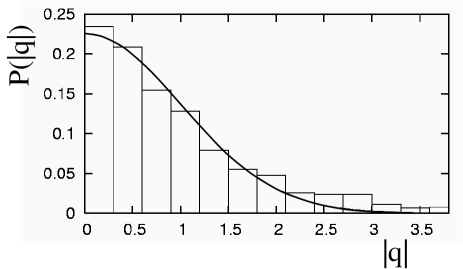
Figure 10: Distribution $P(|q|)$ of the absolute value of the $q$-parameter in Fano resonances found in the transmission eigenvalues $\lambda_{i}$ (the same ensemble of resonances was considered as in Fig. 9). Fitting the data (histograms) with a Gaussian distribution yields good agreement.

Within the limited statistics available, $|q|$ appears to be a Gaussian distributed random variable. Since $q$ is a measure for the ratio of the coupling to the resonant ($r$) scattering channel, relative to the non-resonant continuum ($c$),

$$|q|\propto\frac{|\langle r|t|i\rangle|}{|\langle c|t|i\rangle|}\,,$$ (15)

the distribution $P(|q|)$ peaks near $|\langle r|t|i\rangle|\approx 0$, corresponding to the limit of a “window” resonance. It should be noted that for individual resonances $|q|$ is not invariant under the transformation from the mode representation ($T_{mn}$) to the eigenchannel representation ($\lambda_{i}$). This is because $|q|$ depends explicitly on the ratio of the amplitudes [Eq. (15)] and thus on the matrix elements themselves. Assuming that $|\langle c|t|i\rangle|$ is a smooth, weakly varying function across the resonance, the coupling (or overlap) of the wavefunction of the resonance with the entrance $(|i\rangle)$ channel function can be considered to be a Gaussian random number. Such a hypothesis would agree with RMT predictions for chaotic wavefunctionsMehta (1991) even though there is no a-priori reason for the applicability of RMT to the present hierarchical phase space structure.

V Can fractal conductance fluctuations be observed?

Our calculation extends to mode numbers up to $M=40$ thereby reaching a ratio of $\lambda_{F}/D\lesssim 0.01$. Our calculation reaches therefore further into the semiclassical regime than previous calculations for 2D billiards. It is therefore tempting to probe for the occurrence of fractal conductance fluctuations (FCF) in the transmission probability. According to a semiclassical argumentKetzmerick (1996) quantum dots with mixed classical dynamics can be expected to give rise to self-similar fluctuations (over several orders of magnitude) to which a fractal (i.e. non-integer) dimension can be attributed. Previous numerical results failed to provide unambiguous evidence for the presence of FCF in these systems.Huckestein et al. (2000, 2001); Bäcker et al. (2002); Takagaki and Ploog (2000) This is due to the limited values of $k_{F}$ that could be reached computationally. This difficulty can be circumvented by reducing the two-dimensional scattering devices to effectively one-dimensional systems, so called quantum graph models. Here numerical constraints are less severe thus allowing to explore a regime where both isolated resonances and FCF simultaneously exist.Hufnagel et al. (2001) Our present two-dimensional calculations for transport through the soft-wall stadium (Fig. 1) do not show FCF, even for the highest $k_{F}$ that was accessible by our codes, i.e., $k_{F}\approx 40\times\pi/d$ or $\lambda_{F}/D\approx 0.01$. We attribute the absence of FCF to the fact that even such $k_{F}$ are still too small to probe the turnstiles of the cantori in classical phase space. This statement is supported by our observation that the HDs enter the outermost partial barrier only at resonance energies, i.e. by tunneling. Transport into the inner regions of the hierarchy in phase space seems to be suppressed by the partial barrier. This exploration of hierarchical phase space by way of turnstiles in cantori is, however, crucial for the fractal fluctuations.Ketzmerick (1996)
Our present negative result for soft-wall billiards even for moderately large $k_{F}$ leaves, however, the question open which mechanism is at work that has apparently produced signatures of FCF in several recent experiments.Sachrajda et al. (1998); Micolich et al. (2001, 2002, 2004); Crook et al. (2003) These experiments were in the regime where only a rather limited number of transmitting modes $m,n=2-6$ is open.Micolich et al. (2001) Our results clearly show that the presence of soft walls in the experiment can be ruled out as the source for FCF at moderate $k_{F}$. Note that this observation is in close correspondence to recent findings which suggest that “more complicated processes than those predicted in the semiclassical models are responsible for the observed behavior of FCF”.Micolich et al. (2004)

VI summary

We have investigated the classical and quantum scattering properties for a soft-wall billiard with mixed phase space representing the generic device used in experimental realizations. By analyzing the wave function probability density and the Husimi distribution of scattering states we find remarkable similarities between the classical and quantum phase space structures. This enables us to classify resonant scattering states associated with regular, trapped and instable periodic classical trajectories. Such a mapping of resonant scattering states is mirrored in characteristic differences in the width of the corresponding resonances. Our investigations reveal that the observed resonances in all the partial transmission amplitudes $T_{mn}(k_{F})$ follow the asymmetric Fano lineshape. The distribution of Fano asymmetry parameters $q$ appears to be surprisingly uncorrelated with the injection and ejection angles of the classical trajectories. However, the resonance amplitude is approximately proportional to the geometric mean of the lead mode numbers $\sqrt{m\times n}$. Studying the transmission eigenvalues $\lambda_{i}$ of $\hat{T}=tt^{\dagger}$, we find that Fano resonances in $\lambda_{i}$ feature $q$-parameters following a Gaussian distribution and amplitudes $A_{i}$ that have substantial contributions only in the non-classical transmission eigenchannels.Silvestrov et al. (2003) For numerically accessible wavenumbers with $\lambda_{F}/D\approx 0.01$ fractal conduction fluctuations (FCF) could not be detected.

Acknowledgments

We thank A. Bäcker, L. Hufnagel, F. Libisch, and R. Ketzmerick for helpful discussions. Support by the Austrian Science Foundation (Grant No. FWF-P17359 and No. FWF-P15025) is gratefully acknowledged.

References

- Gutzwiller (1991) M. C. Gutzwiller, Chaos in Classical and Quantum Mechanics (Springer, New York, 1991).
- Markus and Meyer (1974) L. Markus and K. R. Meyer, in Memoirs of the Americal Mathemetical Society (Americal Mathematical Society, Providence, RI, 1974), vol. 114.
- Reed and Kirk (1989) M. A. Reed and W. P. Kirk, eds., Nanostructure Physics and Fabrication (Academic, New York, 1989).
- Lichtenberg and Liebermann (1992) A. J. Lichtenberg and M. A. Liebermann, Regular and Chaotic Dynamics (Springer, New York, 1992), 2nd ed.
- Huckestein et al. (2000) B. Huckestein, R. Ketzmerick, and C. Lewenkopf, Phys. Rev. Lett. 84, 5504 (2000).
- Huckestein et al. (2001) B. Huckestein, R. Ketzmerick, and C. Lewenkopf, Phys. Rev. Lett. 87, 119901(E) (2001).
- Bäcker et al. (2002) A. Bäcker, A. Manze, B. Huckestein, and R. Ketzmerick, Phys. Rev. E 66, 016211 (2002).
- (8) H. Schomerus and C. W. J. Beenakker, Phys. Rev. Lett. 82, 2951 (1999).
- (9) F. Libisch, S. Rotter, J. Burgdörfer, A. Kormányos, and J. Cserti, cond-mat/0504098 (submitted to Phys. Rev. B)
- (10) H.-S. Sim and H. Schomerus, Phys. Rev. Lett. 89, 066801 (2002).
- (11) F. Aigner, S. Rotter, and J. Burgdörfer, cond-mat/0502417 (submitted to Phys. Rev. Lett.)
- (12) E. V. Sukhorukov and O. M. Bulashenko, Phys. Rev. Lett. 94, 116803 (2005).
- Ketzmerick (1996) R. Ketzmerick, Phys. Rev. B 54, 10841 (1996).
- Sachrajda et al. (1998) A. S. Sachrajda, R. Ketzmerick, C. Gould, Y. Feng, P. J. Kelly, A. Delage, and Z. Wasilewski, Phys. Rev. Lett. 80, 1948 (1998).
- Micolich et al. (2001) A. P. Micolich, R. P. Taylor, A. G. Davies, J. P. Bird, R. Newbury, T. M. Fromhold, A. Ehlert, H. Linke, L. D. Macks, W. R. Tribe, et al., Phys. Rev. Lett. 87, 36802 (2001).
- Micolich et al. (2002) A. P. Micolich, R. P. Taylor, A. G. Davies, T. M. Fromhold, H. Linke, L. D. Macks, R. Newbury, A. Ehlert, W. R. Tribe, E. H. Linfield, et al., Appl. Phys. Lett. 80, 4381 (2002).
- Micolich et al. (2004) A. P. Micolich, R. P. Taylor, T. P. Martin, R. Newbury, T. M. Fromhold, A. G. Davies, H. Linke, W. R. Tribe, L. D. Macks, C. G. Smith, et al., Phys. Rev. B 70, 85302 (2004).
- Crook et al. (2003) R. Crook, C. G. Smith, A. C. Graham, I. Farrer, H. E. Beere, and D. A. Ritchie, Phys. Rev. Lett. 91, 246803 (2003).
- Takagaki and Ploog (2000) Y. Takagaki and K. H. Ploog, Phys. Rev. B 61, 4457 (2000).
- Guarneri and Terraneo (2001) I. Guarneri and M. Terraneo, Phys. Rev. E 65, 015203 (2001).
- Benenti et al. (2001) G. Benenti, G. Casati, I. Guarneri, and M. Terraneo, Phys. Rev. Lett. 87, 014101 (2001).
- Budiyono and Nakamura (2003) A. Budiyono and K. Nakamura, Chaos, Solitons and Fractals 17, 89 (2003).
- Louis and Vergés (2000) E. Louis and J. A. Vergés, Phys. Rev. B 61, 13014 (2000).
- Rotter et al. (2000) S. Rotter, J.-Z. Tang, L. Wirtz, J. Trost, and J. Burgdörfer, Phys. Rev. B 62, 1950 (2000).
- Rotter et al. (2003) S. Rotter, B. Weingartner, N. Rohringer, and J. Burgdörfer, Phys. Rev. B 68, 165302 (2003).
- Akis et al. (1997) R. Akis, D. K. Ferry, and J. P. Bird, Phys. Rev. Lett. 79, 123 (1997).
- Heller (1984) E. J. Heller, Phys. Rev. Lett. 53, 1515 (1984).
- Kim et al. (2004) Y.-H. Kim, U. Kuhl, H.-J. Stöckmann, and J. P. Bird, cond-mat/0411331 (2004).
- Fano (1961) U. Fano, Phys. Rev. 124, 1866 (1961).
- Bunimovich (1974) L. A. Bunimovich, Funct. Anal. Appl. 8, 254 (1974).
- Benettin and Strelcyn (1978) G. Benettin and J.-M. Strelcyn, Phys. Rev. A 17, 773 (1978).
- Lin et al. (1993) W. A. Lin, J. B. Delos, and R. V. Jensen, Chaos 3, 655 (1993).
- Meiss and Ott (1986) J. D. Meiss and E. Ott, Physica D 20, 1986 (1986).
- MacKay et al. (1984) R. S. MacKay, J. D. Meiss, and I. C. Percival, Physica (Amsterdam) 13D, 55 (1984).
- Ketzmerick et al. (2000) R. Ketzmerick, L. Hufnagel, F. Steinbach, and M. Weiss, Phys. Rev. Lett. 85, 1214 (2000).
- Bäcker et al. (2004) A. Bäcker, S. Fürstberger, and R. Schubert, Phys. Rev. E. 70, 36204 (2004).
- Bäcker et al. (2005) A. Bäcker, R. Ketzmerick, and A. G. Monastra, Phys. Rev. Lett. 94, 54102 (2005).
- Nöckel and Stone (1994) J. U. Nöckel and A. D. Stone, Phys. Rev. B 50, 17415 (1994).
- Göres et al. (2000) J. Göres, D. Goldhaber-Gordon, S. Heemeyer, M. A. Kastner, H. Shtrikman, D. Mahalu, and U. Meirav, Phys. Rev. B 62, 2188 (2000).
- Rotter et al. (2004a) S. Rotter, F. Libisch, J. Burgdörfer, U. Kuhl, and H.-J. Stöckmann, Phys. Rev. E 69, 46208 (2004a).
- Kobayashi et al. (2002) K. Kobayashi, H. Aikawa, S. Katsumoto, and Y. Iye, Phys. Rev. Lett. 88, 256806 (2002).
- Rotter et al. (2004b) S. Rotter, U. Kuhl, F. Libisch, J. Burgdörfer, and H.-J. Stöckmann, cond-mat/0412544 (2004b).
- Fang and Chang (1998) T. K. Fang and T. N. Chang, Phys. Rev. A 57, 4407 (1998).
- Goldberger and Watson (1964) M. L. Goldberger and K. M. Watson, Collision Theory (Wiley, New York, 1964).
- Ihra (2002) W. Ihra, Phys. Rev. A 66, 020701 (2002).
- (46) M. J. Seaton, Rep. Prog. Phys. 46, 167 (1983).
- (47) H. Friedrich, Theoretical Atomic Physics (Springer, Berlin, 1998).
- Baranger and Mello (1994) H. U. Baranger and P. A. Mello, Phys. Rev. Lett. 73, 142 (1994).
- Jalabert et al. (1994) R. A. Jalabert, J.-L. Pichard, and C. W. J. Beenakker, Europhys. Lett. 27, 255 (1994).
- Wirtz et al. (1997) L. Wirtz, J.-Z. Tang, and J. Burgdörfer, Phys. Rev. B 56, 7589 (1997).
- Silvestrov et al. (2003) P. G. Silvestrov, M. C. Goorden, and C. W. J. Beenakker, Phys. Rev. B 67, 241301(R) (2003).
- (52) Ph. Jacquod, E. V. Sukhorukov, Phys. Rev. Lett. 92, 116801 (2004).
- Mehta (1991) M. L. Mehta, Random Matrices (Academic, New York, 1991).
- Hufnagel et al. (2001) L. Hufnagel, R. Ketzmerick, and M. Weiss, Europhys. Lett. 53, 703 (2001).