Nonlinear response and discrete breather excitation in driven micro-mechanical cantilever arrays.

Abstract

We explain the origin of the generation of discrete breathers (DBs) in experiments on damped and driven micromechanical cantilever arrays (M.Sato et al. Phys. Rev. Lett. 90, 044102, 2003). Using the concept of the nonlinear response manifold (NLRM) we provide a systematic way to find the optimal parameter regime in damped and driven lattices where DBs exist. Our results show that DBs appear via a new instability of the NLRM different from the anticipated modulational instability (MI) known for conservative systems. We present several ways of exciting DBs, and compare also to experimental studies of exciting and destroying DBs in antiferromagnetic layered systems.

The existence and the properties of intrinsic localised modes (ILMs) or discrete breathers (DBs) in nonlinear lattices have been investigated thoroughly during the last years (see DB_rev and references therein). In addition an impressive number of various experiments during the last years have verified the existence of these modes in many systems like micro-mechanical cantilever arrays cant1 ; cant2 , antiferromagnets NatureSievers ; magnet , Josephson junction arrays Trias ; Ustinov , coupled optical waveguides wavegides , atomic vibrations of highly nonlinear materials PtCl ; Ham1 ; Ham2 and Bose-Einstein condensates on optical lattices BEC .

The bulk of the central theoretical results has been achieved for conservative systems. One good reason for that is the complexity of the DB properties. While DBs typically persist under the influence of weak dissipation (which should also include an energy pumping mechanism), various realisations of dissipation (dc driving, ac driving, fluctuations, linear versus nonlinear damping etc) modify DB properties in a specific way, turning the limiting conservative case into an ideal starting playground for setting a coherent frame of the understanding of their properties. Since most of the experimental studies face dissipation, each case may call for a specific additional theoretical study.

DB observation in antiferromagnets NatureSievers ; magnet and cantilever arrays cant1 ; cant2 involved the excitation of the system with spatially homogeneous external fields, triggering a spatially inhomogeneous system state via some inherent instability. For conservative systems the modulational instability (MI) of band edge plane waves is known to provide such a path. Especially for the case of driven cantilevers, the MI approach for conservative systems was used to design an experimental system of alternating short and long cantilevers cant1 ; cant2 . The results we present below show that DBs appear via a completely different instability. The MI can be used for energy pumping and consequent overcoming of dynamical barriers. However several other routes with a similar outcome can be exploited. We demonstrate that by exciting DBs in arrays with identical cantilever length.

In order to study the driven cantilever system we use the model equations in cant1 ; cant2 and introduce the dimensionless time $t\rightarrow t/t_{0}$ and displacement $x_{l}\rightarrow x_{l}/a_{0}$ where $t_{0}$ and $a_{0}$ correspond to a characteristic time and length of the system. The equations of motion describing the cantilever system can be then written as a system of coupled anharmonic damped and ac driven oscillators

$$\ddot{x}_{l}+\gamma\dot{x}_{l}+a_{2}x_{l}+a_{4}x_{l}^{3}-C(x_{l+1}+x_{l-1}-2x_{l})=A(t)$$ (1)

The oscillator displacements $x_{l}$ describe the deflection angle of the $l$-th cantilever from its equilibrium position. The hard-type anharmonicity tends to increase the oscillation frequencies with growing amplitudes. This model neglects the influence of longer than nearest neighbour interaction range, which is not crucial for the understanding of the main qualitative DB properties. The dimensionless parameters are related with the ones of the experiment in ref.cant1 ; cant2 : $\gamma=t_{0}/\tau$, $a_{2}=k_{2}t_{0}^{2}/m$, $a_{4}=k_{4}t_{0}^{2}a_{0}^{2}/m$, $C=k_{l}t_{0}^{2}/m$ and $A=\alpha t_{0}^{2}/a_{0}$. Using the experimental values in cant1 ; cant2 and setting $a_{2}=a_{4}=1$, we find $t_{0}=1.34238\cdot 10^{-6}$sec and $a_{0}=2.46\cdot 10^{-5}$m. The friction and coupling parameters become $\gamma=1.534\cdot 10^{-4}$ and $C=0.07953$. The spatially uniform ac driving $A(t)$ in (1) is generated by a corresponding piezoelectric crystal vibration in the original experiments.

Neglecting the damping $\gamma$, the ac driving $A(t)$ and the nonlinear force terms in (1) one readily derives the only possible solutions, namely plane waves $x_{l}\sim{\rm e}^{i(\omega_{q}t-ql)}$ with the linear dispersion relation $\omega_{q}=\sqrt{1+4C\sin^{2}(q/2)}$ relating the plane wave frequency $\omega_{q}$ to its corresponding wave number $q$. Reinstating the nonlinear force terms in (1) leads to two conclusions DB_rev : i) discrete breathers, i.e. time-periodic and spatially localised solutions $x_{l}(t)=x_{l}(t+T_{b})\;,\;x_{|l|\rightarrow\infty}\rightarrow 0$ exist for frequencies $\Omega_{b}=\frac{2\pi}{T_{b}}>\omega_{q=\pi}$; ii) the $q=\pi$ plane wave mode turns (modulationally) unstable at amplitudes $\sim 1/N$ where $N$ is the number of cantilevers, and DBs bifurcate from this plane wave mode along this very instability route. What can we expect if both damping and ac driving are added as well? DBs persist without much change, thus the ac driving frequency choice $\omega_{d}>\omega_{q=\pi}$ is well reasoned. However instabilities of conservative systems may turn sensitive to effects of damping. Assuming that the MI of the staggered $q=\pi$ mode is the track to follow, the choice of a nonstaggered ac driving is not appropriate. Note that the experimental design of alternating short and long cantilevers splits the spectrum $\omega_{q}$ into two bands separated by a gap. In addition it formally transforms the $q=\pi$ mode of the system with identical cantilevers into the $q=0$ mode of the upper band for the system with alternating cantilever length. Yet the staggered character of this mode is of course preserved inside each unit cell which contains now two neighbouring cantilevers. Thus the mismatch between the staggered MI mode and the nonstaggered ac driving remains also for systems with alternating cantilever length.

With the above parameters $1\leq\omega_{q}\leq 1.1481$. The narrowness of the band as compared to the characteristic frequency values is due to the weak coupling constant $C$. Let us start then from the uncoupled limit. In that case each oscillator evolves independently. Assuming for the moment small amplitudes of all oscillators, the presence of a weak driving will (after some transient time) bring them all into a unique oscillatory state, thus all oscillators will move in phase (with each other). Consequently we have to study the stability of a nonstaggered extended time-periodic state for weak coupling as well, no matter whether the frequency of the driving is located above or below the band $\omega_{q}$.

For a periodic driving of the form $A(t)=A_{0}\cos(\omega_{d}t)$, the equation (1) support periodic solutions. It is easier to study first the properties of these solutions at zero friction ($\gamma=0$), and then examine the modifications when $\gamma\neq 0$. Newton method DB_rev ; ma was used for the tracking of periodic solutions with frequency equal to the external driving of the form: $x_{l}(t)=x_{0,l}\cdot f(\omega_{d}t)$ where $x_{0,l}$ is the amplitude of the oscillation, and $f(\omega_{d}t)$ is a periodic function with period $2\pi$. The Newton scheme was initiated with a very small driving amplitude ($A_{0}\simeq 0$), and the response of the system (i.e. the amplitude of the oscillations $x_{0,l}$) was followed as $A_{0}$ was varying. Thus we reconstruct the full Nonlinear Response Manifold (NLRM) Kopidakis2 .

The NLRM close to the origin follows from linearising the equation of motion (1). The exact solution of the system in this limit is $x_{l}(t)=x_{0,l}\cos(\omega_{d}t)$ with $x_{0,l}=-A_{0}/(\omega_{d}^{2}-1)$. This is a homogeneous branch (HB) (all the oscillators are in phase). There is a phase difference of $\phi=\pi$ between the driving and the response of the system. The NLRM is symmetric around the origin due to $x_{l}(t+\pi/\omega_{d})=-x_{l}(t)$ and $A(t+\pi/\omega_{d})=-A(t)$.

Figure 1: The nonlinear response manifold (NLRM) for $C=0.0079$ and $\omega_{d}=1.3$. Solid line - homogeneous branch, dashed line - various breather branches for $x_{0,0}$. Thick lines correspond to stable parts of the manifold, thin - to unstable ones.

Increasing $|A_{0}|$, the displacement $x_{0,0}$ of HB increase, up to the first turning point (TP) (Fig.1). After the turning point $x_{0,0}$ continue to increase, while the driving amplitude decreases down to zero at the first crossing point (CP1). This crossing point corresponds to a homogenous solution with all the oscillators are oscillating with the same amplitude $x_{0,0}$ and zero driving. This state exists due to the frequency increasing, hard anharmonicity term in the equations of motion and because $\omega_{d}>\omega_{q}$. The NLRM manifold of the HB continues further from CP1 with again nonzero $A_{0}$, but the solution is now in phase with the driving.

The Floquet stability analysis DB_rev of the HB reveals that close to the origin the manifold is linearly stable. An instability appear before the TP and the HB becomes unstable. The NLRM of the homogeneous branch continues to be unstable between the TP and the CP1. After the CP1, the homogeneous branch turns stable again (see Fig.1).

Figure 2: (a,b) The NLRM for different values of the driving frequency: (a) $\omega_{d}=1.2$, (b) $\omega_{d}=1.4$. The parameters are the same used in Fig.1. (c,d) the response $x_{0,0}$ and the phase difference $\phi$ of the manifold in the neighbourhood of the first crossing point for different values of the friction. Continuous line corresponds to $\gamma=0$, dotted line to $\gamma=0.001$ and dashed line to $\gamma=0.005$.

The instabilities of the HB mark the bifurcation of spatially inhomogeneous solutions - various breather states - off the HB. For a system of $N$ oscillators, at the first instability, $N$ new branches of the NLRM appear. Each of these branches corresponds to a single breather centred at a different site on the lattice. In Fig.1 we show two of these branches with dashed lines. Starting from the bifurcation, the displacement of the central oscillator increases, while $|A_{0}|$ decreases. For $A_{0}=0$ the manifold passes through the second crossing point (CP2). This branch of the manifold corresponds to a breather, and is stable for $A_{0}>0$ and unstable for $A_{0}<0$. After that, the manifold turns, and passes through further crossing points. Thus for fixed $\omega_{d}$ we have multistability for small enough $A_{0}$ with a large amplitude and small amplitude HB coexisting together with breather states. For large enough $A_{0}$ only the large amplitude HB survives.

The NLRM depends on the driving frequency $\omega_{d}$. In Fig.2 we show a part of the NLRM for two different values of the driving frequency. In Fig.2(a) $\omega_{d}=1.2$ and in Fig.2(b) $\omega_{d}=1.4$. With increasing frequency the slope of the manifold decreases, the crossing points appear for larger values of $x_{0,0}$, as a result the bifurcations and the turning points appear for larger values of $|A_{0}|$.

The properties of the manifold are slightly modified due to the presence of friction ($\gamma\neq 0$).

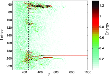
Figure 3: Energy as a function of time. The driving frequency is initially ramped from $\omega_{d}=1.14$ to $\omega_{d}=1.4$, and then it remains fixed (marked by the vertical dashed line). Energy pumping is observed during the ramping. At the end of the ramping process, breathers are created, and one of them locks to the driving and survives. $T_{1}=20\pi/\omega_{d}$.

The NLRM between the origin and the crossing point (CP1) for $\gamma=0$ is in anti-phase with the driving, while after the crossing point the NLRM is in phase with the driving. For $\gamma=0$ therefore there is a phase difference of $\phi=\pi$ in the response of the system around a CP. When a small friction is introduced in the system, it creates an extra small phase difference between the driver and the response. This phase difference between the driving and the response increases in the neighbourhood of the CP. The result is that the solution at the CP disappears due to friction, but there is a smooth transition between the two different branches of the manifold. The phase difference $\phi$ varies smoothly from $\pi-\epsilon_{-}$ to $0+\epsilon_{+}$ where $\epsilon_{\pm}$ correspond to the small phase differences created by the friction on the large and low amplitude branch respectively, far from the CP. For weak damping this transition occurs very close to the CP. The smooth transition between the two branches of the manifold in the neighbourhood of (CP1) as a function of $|A_{0}|$ is shown in Fig.2(c) for different values of the friction. The smooth transition in the phase difference $\phi$ is shown in Fig.2(d).

Figure 4: (a) Average energy per oscillator as a function of time (solid line, scaled by a factor of 10 for better observation) and the energy of the locked oscillator (strongly fluctuating dotted line). The parameters and the frequency ramping are like in Fig.3. (b) The frequency ramping scheme. After the vertical dashed line the driving frequency remains constant.

Far from the CP, the properties of the manifold are only slightly modified by the nonzero friction.

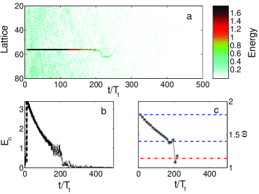
Figure 5: (a) Energy density evolution for a sequence of different driving (see text for details); (b) Time dependence of the DB energy observed in (a); (c) Time dependence of the DB frequency observed in (a). The two dashed lines mark the frequencies $\omega_{1}$ and $\omega_{2}$. The dashed-dotted line corresponds to band edge frequency $\omega_{\pi}$.

As follows from Fig.2, the stable breather branch is not connected to the stable HB of the NLRM. Thus we can exclude an easy way of exciting the system in the HB and tuning some parameter (amplitude or frequency of the driving) such that we continuously join the breather branch. This calls for stochastic excitations of the system to enforce a nonzero probability to end up in a breather state when initially starting from a HB. Similar to the experiments cant1 ; cant2 we performed a ramping of the frequency $\omega_{d}$ from 1.14 (inside the band) to 1.4 (above the band) for fixed amplitude $A_{0}=0.008$ (cf. Fig.4(b)). According to Fig.2 the final state corresponds to the multistability domain of the NLRM. If the system was initially at rest, the final state is observed to be the low amplitude HB. However, adding some nonzero noise, uniformly distributed in the interval $(-0.05,0.05)$, in the initial conditions of the cantilever deflection angles, the ramping process excites a unstable plane wave, which provides a finite time energy pumping due to MI (Fig.3). The MI acts as a noise amplifier, which allows for the generation of hot spots or breather precursors. After the ramping finishes, most of these hot spots decay back into the low amplitude HB, while some of them may lock to the driver and turn into a stable breather. The average energy per oscillator is shown in Fig.4(a) as a function of time. During the ramping, there is a frequency window, where energy is pumped into the system, and then the system relaxes due to dissipation. The dotted line shows the energy of the locked breather site.

In order to verify that the energy pumping mediated by the MI in the experiments is only needed to amplify the noise, we perform simulations in the absence of a frequency ramping, but with the initial fluctuations being larger (Gaussian distribution of initial displacements with zero mean and variance $D=0.5$). Keeping the frequency and the driving amplitude fixed ($\omega_{d}=1.4$ and $A_{0}=0.008$) we observe the creation and locking of breathers similar to Fig.5. Similar simulations with alternating long and short cantilevers, reveal the same behaviour.

The NLRM study shows, that breathers can be obtained in a driven and damped system by carefully choosing the frequency (outside the phonon band) and amplitude of the driving force (not being too large) such that the NLRM is activated inside the multistability domain. We have shown that localised breathers emerge from the homogeneous solution via an instability of the NLRM completely different from the expected MI picture. The fact that the stable breather branch is disconnected from the stable HB, implies that fluctuations have to be used in order to perform a crossover from one to the other. There exist various pathways of generating breathers, either by frequency ramping and exploiting the MI, or by initially strongly exciting the system. These pathways have to be designed in such a way that the system will tend to the small amplitude HB of the NLRM, with some fluctuations growing into hot spots which finally transform into breather states.

The NLRM can be also used to study the breather excitation in antiferromagnetic systems NatureSievers ; magnet where external driving was used as well. The observed breather destruction in these experiments is similar to the process presented in Fig.5. In analogy with the experiment a strong driving at frequency $\omega_{1}=1.8$ with $A_{1}=0.8$ and duration of $t=20T_{1}$ is used, together with initial displacements being uniformly distributed in the interval $(-0.25,0.25)$. As a result a DB is formed (Fig5(a)). A subsequent long driving at a frequency $\omega_{2}=1.4$ (being located closer to the spectrum $\omega_{q}$) is exciting the system with a small amplitude $A_{2}=0.008$. Because of the frequency mismatch the breather with $\omega_{1}$ will start to decay, but tend to slow down the decay when its frequency is close to $\omega_{2}$ (Fig5(c)). Similar to the experimental case we add a third weak driving signal with $\omega_{3}=2$ and amplitude $A_{3}=0.0004$. That hinders the locking of the DB to $\omega_{2}$. Right after the DB frequency passes $\omega_{2}$, its relaxation speeds up and the excitation is destroyed very quickly (Fig.5(b), cf. also Fig.3 in NatureSievers . The observed energy release is fixed by the energy value of a DB locked to the $\omega_{2}$ driving and explains the experimental observation of equal height steps in the relaxation of DBs. At the same time we interprete the observed smooth decrease of the emission signal in Fig.3 in NatureSievers as a process of slow relaxation of DBs with frequency $\omega_{1}$ towards DBs with frequency $\omega_{2}$.

Acknowledgements. We thank A. J. Sievers and U. Schwartz for helpful discussions.

References

- (1) S. Aubry, Physica D 103, 201 (1997); S. Flach, C.R. Willis, Phys. Rep. 295, 181 (1998); Energy Localisation and Transfer, edited by T. Dauxois, A. Litvak-Hinenzon, R. MacKay and A. Spanoudaki (World Scientific, Singapore, 2004); D. K. Campbell, S. Flach and Yu. S. Kivshar, Physics Today 57(1), 43 (2004).
- (2) M. Sato, B. E. Hubbard, A. J. Sievers, B. Ilic, D. A. Czaplewski and H. G. Craighead, Phys. Rev. Lett. 90, 044102 (2003).
- (3) M. Sato, B. E. Hubbard, L. Q. English, A. J. Sievers, B. Ilic, D. A. Czaplewski and H. G. Craighead, Chaos 13, 702 (2003).
- (4) M. Sato and A. J. Sievers, Nature 432, 486 (2004).
- (5) U. T. Schwarz, L. Q. English and A. .J. Sievers, Phys. Rev. Lett. 83, 223 (1999).
- (6) E. Trias, J. Mazo and T. Orlando, Phys. Rev. Lett. 84, 741 (2000).
- (7) P. Binder, D. Abraimov, A. V. Ustinov, S. Flach and Y. Zolotaryuk, Phys. Rev. Lett. 84, 745 (2000).
- (8) H. S. Eisenberg, Y. Silberberg, R. Morantotti, A. R. Boyd and J. S. Atchinson, Phys. Rev. Lett. 81, 3383 (1998).
- (9) B. I. Swanson, J. A. Brozik, S. P. Love, G. F. Strouse, A. P. Shreve, A. R. Bishop, W. Z. Wang and M. I. Salkola, Phys. Rev. Lett. 82, 3288 (1999).
- (10) J. Edler, P. Hamm and A. C. Scott, Phys. Rev. Lett. 88, 067403 (2002).
- (11) J. Edler and P. Hamm, J. Chem. Phys. 117, 2415 (2002).
- (12) B. Eiermann, Th. Anker, M. Albiez, M. Taglieber, P. Treutlein, K. P. Marzlin and M. K. Oberthaler, Phys. Rev. Lett. 92, 230401 (2004).
- (13) J. L. Marin and S. Aubry, Nonlinearity 9, 1501 (1994).
- (14) G. Kopidakis and S. Aubry, Physica D 130, 155 (1999); Physica D 139, 247 (2000); Phys. Rev. Lett. 84, 3236 (2000).