NMR relaxation time in a clean two-band superconductor

Abstract

We study the spin-lattice relaxation rate of nuclear magnetic resonance in a two-band superconductor. Both conventional and unconventional pairing symmetries for an arbitrary band structure in the clean limit are considered. The importance of the inter-band interference effects is emphasized. The calculations in the conventional case with two isotropic gaps are performed using a two-band generalization of Eliashberg theory.

I Introduction

Although the Fermi surface in most superconductors consists of more than one sheet, this does not necessarily mean that all those materials are multi-band superconductors. The true multi-band (in particular two-band) superconductivity is in fact a rather uncommon phenomenon characterized by a significant difference in the order parameter magnitudes in different bands. For this to be the case, the system has to satisfy some quite stringent requirements, namely the pairing interactions and/or the densities of states should vary considerably between the bands and the inter-band processes, e.g. due to impurity scattering, should be weak. Although some examples have been known since early 1980s,Binnig80 the recent swell of interest in this subject has been largely stimulated by the discovery of two-band superconductivity in MgB₂.MgB2 Most of the experimental evidence, see Ref. MgB2-review, and the references therein, support the conclusion that there are two distinct superconducting gaps $\Delta_{\pi}$ and $\Delta_{\sigma}$ in this material, with $\Delta_{\sigma}/\Delta_{\pi}\simeq 2.63$.Golub02 (There are actually four bands crossing the Fermi level in MgB₂, which can be grouped into 2 quasi-two-dimensional $\sigma$-bands and 2 three-dimensional $\pi$-bands and described by an effective two-band model.) Other candidates for multi-band superconductivity which have emerged recently include nickel borocarbides,CGB98 NbSe₂,NbSe2 and also the heavy-fermion compounds CeCoIn₅ (Ref. CeCoIn5, ) and CePt₃Si (Ref. CePtSi, ). It seems more likely to find a two-band superconductivity in unconventional materials, since they are intrinsically in a clean limit, so at least the gap averaging due to impurity scattering is not effective.

Theoretically, a two-band generalization of the Bardeed-Cooper-Schrieffer (BCS) model was introduced independenly by Suhl, Matthias, Walker,SMW59 and Moskalenko.Moskal59 In subsequent developments, many aspects of the multi-band model have been studied, including the thermodynamic and transport properties, the effects of impurities and strong coupling, etc.GZK67 ; Chow68 ; Ent76 ; SS77 Surprisingly, little attention has focussed on such an important characteristic as the spin-lattice relaxation rate $T_{1}^{-1}$ of nuclear magnetic resonance (NMR). The measurements of $T_{1}^{-1}$ probe the properties of the electron subsystem which are local in real space and therefore extremely non-local in the momentum space.Slichter90 In the presence of multiple Fermi-surface sheets this would give rise to inter-band interference terms in $T_{1}^{-1}$, even without any inter-band scattering due to interactions or impurities. The inter-band terms in $T_{1}^{-1}$ are not negligible and can be expected to strongly affect the temperature dependence of the relaxation rate compared to the single-band case.HS59

The purpose of this article is to calculate the nuclear spin relaxation rate in a two-band superconductor, for both conventional and unconventional types of pairing. We focus on singlet pairing in the absence of impurities, assuming that the relaxation is dominated by the Fermi contact interaction between the nucleus and the conduction electrons. The article is organized as follows. In Sec. II, we develop a general formalism based on an anisotropic two-band BCS model and show that, while the resulting expressions in the unconventional case are well-defined and can be calculated without any additional complications, in the conventional isotropic case one encounters divergent integrals. In Sec. III, we single out the isotropic case for a strong-coupling theory treatment, in which the divergences are smeared out due to the quasiparticle lifetime effects. In Sec. IV, we apply the general theory to the relaxation rate on the ²⁵Mg site in MgB₂ using the realistic strong-coupling parameters.

II Weak coupling theory

Without the loss of generality, we consider the case of a nuclear spin $I=1/2$ located at the origin of the crystal lattice. Higher values of $I$ change only the overall pre-factor in the expression for the relaxation rate,Slichter90 which drops out of the ratio of the relaxation rates in the superconducting and the normal states. The spin-lattice relaxation rate due to the hyperfine contact interaction of the nucleus with the band electrons is given by

$$R\equiv\frac{1}{T_{1}T}=-\frac{J^{2}}{2\pi}\lim\limits_{\omega_{0}\to 0}\frac{\,\mathrm{Im}\,K^{R}_{+-}(\omega_{0})}{\omega_{0}},$$ (1)

where $J$ is the hyperfine coupling constant, $\omega_{0}$ is the NMR frequency, and $K^{R}_{+-}(\omega_{0})$ is the Fourier transform of the retarded correlator of the electron spin densities at the nuclear site:

$$K_{+-}^{R}(t)=-i\left\langle\left[S_{+}(\bm{0},t),S_{-}(\bm{0},0)\right]\right\rangle\theta(t).$$ (2)

Here $S_{\pm}(\bm{r},t)=e^{iH_{e}t}S_{\pm}(\bm{r})e^{-iH_{e}t}$, $H_{e}$ is the electron Hamiltonian, and

$$S_{+}(\bm{r})=\psi^{\dagger}_{\uparrow}(\bm{r})\psi_{\downarrow}(\bm{r}),\quad S_{-}(\bm{r})=\psi^{\dagger}_{\downarrow}(\bm{r})\psi_{\uparrow}(\bm{r})$$ (3)

($\hbar=k_{B}=1$ in our units, and the spin quantization axis is along the external magnetic field $\bm{H}$). The derivation of Eq. (1) is outlined in Appendix A. The retarded correlator is obtained by analytical continuation of the Matsubara time-ordered correlator: $K^{R}_{+-}(\omega)=K(\nu_{m})|_{i\nu_{m}\to\omega_{0}+i0^{+}}$, with $\nu_{m}=2\pi mT$.

We assume that there are two spin-degenerate electron bands in the crystal (the generalization to an arbitrary number of bands is straightforward), and neglect the spin-orbit coupling. The two-band generalization of the BCS Hamiltonian reads $H_{e}=H_{0}+H_{int}$,SMW59 where

$$H_{0}=\sum\limits_{i,\bm{k}\alpha}\xi_{i,\bm{k}}c^{\dagger}_{i,\bm{k}\alpha}c_{i,\bm{k}\alpha}$$ (4)

is the non-interacting part ($i=1,2$ is the band index, $\alpha=\uparrow,\downarrow$ is the spin projection, and the chemical potential $\mu$ is included in the band dispersion), and $H_{int}=H^{(1)}_{int}+H^{(2)}_{int}+H^{(12)}_{int}$ is the pairing interaction. For anisotropic singlet pairing, we have

$$H^{(i)}_{int}=\frac{1}{2}\sum\limits_{\bm{k},\bm{k}^{\prime}}V_{ii}(\bm{k},\bm{k}^{\prime})c^{\dagger}_{i,\bm{k}\uparrow}c^{\dagger}_{i,-\bm{k}\downarrow}c_{i,-\bm{k}^{\prime}\downarrow}c_{i,\bm{k}^{\prime}\uparrow}$$

$$H^{(12)}_{int}=\frac{1}{2}\sum\limits_{\bm{k},\bm{k}^{\prime}}V_{12}(\bm{k},\bm{k}^{\prime})c^{\dagger}_{1,\bm{k}\uparrow}c^{\dagger}_{1,-\bm{k}\downarrow}c_{2,-\bm{k}^{\prime}\downarrow}c_{2,\bm{k}^{\prime}\uparrow}$$

$$+\mathrm{H.c.}$$ (5)

The Hamiltonians $H^{(1)}_{int}$ and $H^{(2)}_{int}$ describe the intra-band pairing of electrons, while $H^{(12)}_{int}$ describes the pair scattering between the bands. The inter-band interactions of the form $c^{\dagger}_{1,\bm{k}\uparrow}c^{\dagger}_{2,-\bm{k}\downarrow}c_{2,-\bm{k}^{\prime}\downarrow}c_{1,\bm{k}^{\prime}\uparrow}$ are suppressed if the band splitting is large compared to all energy scales relevant to superconductivity. We assume, following Hebel and Slichter HS59 that, while the resonance is observed in a strong field in the normal state, the relaxation takes place in a uniform superconducting state after switching off the field.

The pairing symmetry is the same in both bands and is determined by one of the irreducible representations, $\Gamma$, of the point group of the crystal. The functions $V_{ij}(\bm{k},\bm{k}^{\prime})$ are non-zero only in a thin energy shell near the Fermi surfaces and can be represented in a factorized form:

$$V_{ij}(\bm{k},\bm{k}^{\prime})=V_{ij}\sum_{a=1}^{d_{\Gamma}}\varphi_{a}(\bm{k})\varphi_{a}(\bm{k}^{\prime}),$$ (6)

where $\varphi_{a}(\bm{k})$ are the basis functions, and $d_{\Gamma}$ is the dimensionality of $\Gamma$. In the absence of time-reversal symmetry breaking $\varphi_{a}$’s can be chosen real. The basis functions do not have to be the same in both bands, but we neglect this complication here.

The properties of our superconductor can be described using a standard field-theoretical formalism in terms of the normal and anomalous Gor’kov functions:AGD63

$$G_{i,\alpha\beta}(\bm{k},\tau)=\delta_{\alpha\beta}G_{i}(\bm{k},\tau),$$

$$F_{i,\alpha\beta}(\bm{k},\tau)=(i\sigma_{2})_{\alpha\beta}F_{i}(\bm{k},\tau),$$

$$F^{\dagger}_{i,\alpha\beta}(\bm{k},\tau)=(-i\sigma_{2})_{\alpha\beta}F^{\dagger}_{i}(\bm{k},\tau),$$

which can be combined into a $2\times 2$ matrix Green’s function

$$\hat{G}_{i}(\bm{k},\tau)=\left(\begin{array}[]{cc}G_{i}(\bm{k},\tau)&-F_{i}(\bm{k},\tau)\\ -F^{\dagger}_{i}(\bm{k},\tau)&-G_{i}(-\bm{k},-\tau)\\ \end{array}\right).$$ (7)

In the mean-field approximation, the interaction Hamiltonian is reduced to the form

$$H_{int}=\frac{1}{2}\sum\limits_{i,\bm{k}}\Delta_{i,\bm{k}}c^{\dagger}_{i,\bm{k}\uparrow}c^{\dagger}_{i,-\bm{k}\downarrow}+\mathrm{H.c.},$$ (8)

where $\Delta_{i,\bm{k}}$ is the superconducting order parameter in the $i$th band, which can be written as

$$\Delta_{i,\bm{k}}=\sum\limits_{a}\eta_{i,a}\varphi_{a}(\bm{k}),$$ (9)

with $\eta_{i,a}$ being the order parameter components. Both order parameters appear at the same critical temperature $T_{c}$, but have different temperature dependences, which can be found by solving a system of $2d_{\Gamma}$ self-consistency equations for the functions $\eta_{i,a}(T)$. In the frequency representation, the Green’s functions (7) become

$$\hat{G}_{i}(\bm{k},\omega_{n})=-\frac{i\omega_{n}\tau_{0}+\xi_{i,\bm{k}}\tau_{3}+\hat{\Delta}_{i,\bm{k}}}{\omega_{n}^{2}+\xi_{i,\bm{k}}^{2}+|\Delta_{i,\bm{k}}|^{2}},$$ (10)

where $\tau_{i}$ are Pauli matrices, $\omega_{n}=(2n+1)\pi T$, and

$$\hat{\Delta}_{i,\bm{k}}=\left(\begin{array}[]{cc}0&\Delta_{i,\bm{k}}\\ \Delta^{*}_{i,\bm{k}}&0\\ \end{array}\right).$$ (11)

Now we return to the calculation of the relaxation rate (1). For zero spin-orbit coupling, the spin operators (3) can be written in the band representation, using

$$\psi_{\alpha}(\bm{r})=\frac{1}{\sqrt{V}}\sum\limits_{i,\bm{k}}e^{i\bm{k}\bm{r}}u_{i,\bm{k}}(\bm{r})c_{i,\bm{k}\alpha},$$ (12)

where $u_{i,\bm{k}}(\bm{r})$ are the Bloch functions, which are periodic in the unit cell, and $V$ is the system volume. Inserting these into Eqs. (3), one obtains the Matsubara spin correlator $K(\tau)=-\langle T_{\tau}S_{+}(\bm{0},\tau)S_{-}(\bm{0},0)\rangle$, which can be decoupled in the mean-field approximation, using the Green’s functions (7). In the absence of time-reversal symmetry breaking, one can show that $u_{i,-\bm{k}}(\bm{0})=u_{i,\bm{k}}^{*}(\bm{0})$. Then, taking the thermodynamic limit, we have

$$K(\nu_{m})=\frac{1}{2}T\sum\limits_{n}\int\limits_{\bm{k}_{1,2}}\,\mathrm{Tr}\,[\hat{\cal G}(\bm{k}_{1},\omega_{n}+\nu_{m})\hat{\cal G}(\bm{k}_{2},\omega_{n})],$$ (13)

where

$$\int\limits_{\bm{k}}(...)=\lim\limits_{V\to\infty}\frac{1}{V}\sum\limits_{\bm{k}}(...)=\int\frac{d^{D}k}{(2\pi)^{D}}(...),$$

and

$$\hat{\cal G}(\bm{k},\omega_{n})=\sum\limits_{i}|u_{i,\bm{k}}(\bm{0})|^{2}\hat{G}_{i}(\bm{k},\omega_{n}),$$ (14)

with $\hat{G}_{i}(\bm{k},\omega_{n})$ given by Eq. (10).

Calculating the matrix traces and the Matsubara sums in Eq. (13) followed by the analytical continuation to real frequencies, we find that the imaginary part of $K^{R}_{+-}(\omega)$ is proportional to $\omega$ at $\omega\to 0$. The momentum integrals are calculated making the usual assumption that $u_{i,\bm{k}}(\bm{0})$ and $\Delta_{i,\bm{k}}$ weakly depend on $\xi_{i,\bm{k}}$ in the vicinity of the Fermi surface (i.e. within the energy range of the order of $T$). We introduce the local density of quasiparticle states at $\bm{r}=\bm{0}$: $N(\omega)=N_{1}(\omega)+N_{2}(\omega)$ ($\omega>0$), where

$$N_{i}(\omega) = \frac{1}{2}\int\limits_{\bm{k}}|u_{i,\bm{k}}(\bm{0})|^{2}\delta(\omega-E_{i,\bm{k}})$$ (15)

$$= N_{F,i}\left\langle|u_{i,\bm{k}}(\bm{0})|^{2}\frac{\omega}{\sqrt{\omega^{2}-|\Delta_{i,\bm{k}}|^{2}}}\right\rangle_{i},$$

where $E_{i,\bm{k}}=\sqrt{\xi^{2}_{i,\bm{k}}+|\Delta_{i,\bm{k}}|^{2}}$ is the Bogoliubov excitation energy in the $i$th band, the angular brackets stand for the average over the Fermi surface, and $N_{F,i}=(1/8\pi^{3})\int dS_{F}/|\bm{v}_{F,i}|$ is the density of states at the Fermi level in the $i$th band. The angular integration in Eq. (15) is restricted by the condition $|\Delta_{i,\bm{k}}|\leq\omega$. We also introduce the function $M(\omega)=M_{1}(\omega)+M_{2}(\omega)$, where

$$M_{i}(\omega) = \frac{1}{2}\int\limits_{\bm{k}}\frac{\Delta_{i,\bm{k}}}{E_{i,\bm{k}}}|u_{i,\bm{k}}(\bm{0})|^{2}\delta(\omega-E_{i,\bm{k}})$$ (16)

$$= N_{F,i}\left\langle|u_{i,\bm{k}}(\bm{0})|^{2}\frac{\Delta_{i,\bm{k}}}{\sqrt{\omega^{2}-|\Delta_{i,\bm{k}}|^{2}}}\right\rangle_{i}.$$

Then,

$$R=J^{2}\int\limits_{0}^{\infty}d\omega\left(-\frac{\partial f}{\partial\omega}\right)\left[N^{2}(\omega)+|M(\omega)|^{2}\right],$$ (17)

where $f(\omega)=(e^{\omega/T}+1)^{-1}$ is the Fermi function.

For $\Delta_{i}(\bm{k})=0$, we have $M(\omega)=0$, and the normal-state relaxation rate is given by $R_{n}=J^{2}N_{n}^{2}/2$, where $N_{n}=N_{n,1}+N_{n,2}$,

$$N_{n,i}=N_{F,i}\left\langle|u_{i,\bm{k}}(\bm{0})|^{2}\right\rangle_{i}.$$ (18)

Finally, we obtain for the ratio of the NMR relaxation rates in the superconducting and the normal states

$$\frac{R_{s}}{R_{n}}=2\int\limits_{0}^{\infty}d\omega\left(-\frac{\partial f}{\partial\omega}\right)\frac{N^{2}(\omega)+|M(\omega)|^{2}}{N_{n}^{2}}.$$ (19)

As we pointed out at the beginning of this Section, our result does not depend on the nuclear spin $I$. The expression (19) has two notable properties. First, the relaxation rate is controlled by the local densities of quasiparticle states. Only in the limit of a single-band isotropic pairing can one express $R$ in terms of the total density of states and recover the Hebel-Slichter formula,HS59 see Sec. II.1 below. Second, the contributions to the spin-lattice relaxation rate from different bands are not simply additive, since there are inter-band interference terms in Eq. (19). These terms are present even in the absence of any inter-band interactions or impurity scattering and can be traced back to the local character of the hyperfine coupling $\bm{I}\bm{S}$, which mixes together the electron states near the Fermi surface from different bands.

II.1 Conventional pairing

The order parameter is “conventional” if it transforms according to the unity representation of the point group $\Gamma$.Book The gap functions $\Delta_{i,\bm{k}}$ can be isotropic or anisotropic, with $M_{s}(\omega)\neq 0$ in both cases.

Assuming the isotropic pairing with a uniform order parameter, we have $\Delta_{i,\bm{k}}=\Delta_{i}$, where both gap functions can be chosen real without loss of generality. One can view this as an extreme case of anisotropic superconductivity on an extended single sheet of the Fermi surface, in which the gap function is allowed to take only two values, $\Delta_{1}$ and $\Delta_{2}$. The densities of states become

$$N(\omega)=\sum\limits_{i}N_{n,i}\frac{\omega}{\sqrt{\omega^{2}-\Delta_{i}^{2}}},$$ (20)

$$M(\omega)=\sum\limits_{i}N_{n,i}\frac{\Delta_{i}}{\sqrt{\omega^{2}-\Delta_{i}^{2}}}.$$ (21)

Substituting these expressions in Eq. (19) we arrive at a logarithmically divergent integral. The origin of this divergence is the same as in the Hebel-Slichter formula in the single-band case:HS59 one has to square the BCS-like density of quasiparticle states, which is singular at $E=\Delta_{1},\Delta_{2}$. Allowing for a non-zero NMR frequency $\omega_{0}$ yields the relaxation rate which is still much higher than that observed in experiment.Tink96

One can smear out the singularity and cut off the divergence either by introducing some gap anisotropy,Masuda62 or by taking into account the strong-coupling effects, which lead to a finite lifetime of quasiparticles and therefore to energy-dependent complex gap functions.Fibich65 Which mechanism is more important depends on the material. In Sec. III below, we adopt the latter point of view and derive the strong-coupling expression for the relaxation rate for an isotropic gap.

II.2 Unconventional pairing

If the order parameter transforms according to a non-unity representation of the point group, then it follows from the obvious property of the Bloch functions $|u_{i,g\bm{k}}(\bm{0})|^{2}=|u_{i,\bm{k}}(\bm{0})|^{2}$ ($g$ is an arbitrary element of the point group) that $M(\omega)=0$. Therefore,

$$\frac{R_{s}}{R_{n}}=2\int\limits_{0}^{\infty}d\omega\left(-\frac{\partial f}{\partial\omega}\right)\left[\frac{N_{1}(\omega)+N_{2}(\omega)}{N_{n,1}+N_{n,2}}\right]^{2},$$ (22)

where $N_{i}(\omega)$ and $N_{n,i}$ are defined by Eqs. (15) and (18) respectively. In most cases the integral converges, because the square-root singularity in the density of states is smeared out by the intrinsic anisotropy of the gap. The only exception is an unconventional order parameter with isotropic gap (e.g. an analog of the $B$-phase of ³He in a charged isotropic superfluid), in which case the integral is again logarithmically divergent.

Since the inter-band pair scattering $H^{(12)}_{int}$ in Eq. (II) induces the order parameters of the same symmetry in both bands, the low-energy behavior of $N_{1}(\omega)$ and $N_{2}(\omega)$ is characterized by the same power law. If there are line (point) nodes in the gap, then $N_{1,2}(\omega)\propto\omega$ $(\omega^{2})$ at $\omega\to 0$, Book and $R\propto T^{2}$ $(T^{4})$ as $T\to 0$.SU91 ; Hase96 This behavior has indeed been observed in most heavy-fermion compounds, for a recent review see Ref. Flouq05, .

This picture will change if the gap magnitudes in the bands are considerably different (as mentioned in the Introduction, there are indications that this might be the case in such materials as CeCoIn₅ and CePt₃Si). For example, if the gap in one band is much smaller than in the other, then, taking the limit $\Delta_{2,\bm{k}}\to 0$, one obtains instead of Eq. (22)

$$\frac{R_{s}}{R_{n}} = 2\int\limits_{0}^{\infty}d\omega\left(-\frac{\partial f}{\partial\omega}\right)$$ (23)

$$\times\frac{N^{2}_{1}(\omega)+2N_{1}(\omega)N_{n,2}+N^{2}_{n,2}}{(N_{n,1}+N_{n,2})^{2}}.$$

While the last term in the integral contributes to the residual relaxation rate at $T=0$, it is the second term that controls the power-law behavior at low $T$: we now have $R={\rm const}+aT$ for line nodes, and $R={\rm const}+aT^{2}$ for point nodes.

As an illustration of the above results, let us consider a simple example of a quasi-two-dimensional two-band superconductor with circular Fermi surfaces and a $d$-wave gap $\Delta_{1,\bm{k}}=\Delta_{0}\cos 2\theta$, which has vertical lines of nodes. The fraction of the density of states from the electrons in the unpaired band is $r=N_{n,2}/(N_{n,1}+N_{n,2})$. The Fermi-surface average in Eq. (15) can be done analytically:

$$\frac{N_{1}(\omega)}{N_{n,1}}=\frac{2}{\pi}\left\{\begin{array}[]{cc}\displaystyle xK(x^{2})&,\ {\rm if}\ x\leq 1,\\ \displaystyle K(x^{-2})&,\ {\rm if}\ x>1,\end{array}\right.$$ (24)

where $x=\omega/\Delta_{0}$, and $K(x)$ is the complete elliptic integral of the first kind.AS65

In Fig. 1, we show the results of the numerical calculation of the temperature dependence of the relaxation rate (23) for different values of $r$. Instead of determining the exact temperature dependence of $\Delta_{0}$ at all $T$, which would involve a full numerical solution of the self-consistency gap equation, we use the approximate expression $\Delta_{0}(T)/\Delta_{0}(0)=\sqrt{1-(T/T_{c})^{3}}$, where $\Delta_{0}(0)/k_{B}T_{c}=1.30$ (this number is obtained from the solution of the gap equation at $T=0$). For $r=0$, one recovers the limit of a single-band $d$-wave superconductor with $R\propto T^{2}$ at low $T$ and a small Hebel-Slichter peak immediately below $T_{c}$. As $r$ grows, so do both the deviation from the $T^{2}$ behavior and the residual relaxation rate at $T=0$. One interesting observation is that even if the density of states is dominated by the contribution from the unpaired sheet of the Fermi surface, one still can see an appreciable suppression of the relaxation rate at low temperatures.

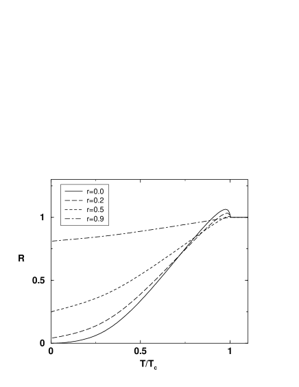
Figure 1: The NMR relaxation rate in a two-band superconductor with lines of nodes in one band and a negligible gap in the other, for different values of $r=N_{n,2}/(N_{n,1}+N_{n,2})$.

III Strong coupling theory

In this section we generalize the results of the weak coupling theory, Sec. II, to the case of an electron-phonon multi-band superconductor which could be described by Eliashberg-type equations.Ent76 ; Golub02 To include the self-energy effects associated with both electron-phonon and screened Coulomb interaction one replaces Eq. (13) with

$$K(\nu_{m})=\frac{1}{2}T\sum\limits_{n}\int\limits_{\bm{k}_{1,2}}\sum_{i,j}|u_{i,\bm{k}_{1}}(\bm{0})|^{2}|u_{j,\bm{k}_{2}}(\bm{0})|^{2}$$

$$\times\,\mathrm{Tr}\,[\hat{G}_{i}(\bm{k}_{1},\omega_{n})\hat{\Gamma}_{ij}(\bm{k}_{1},\bm{k}_{2};\omega_{n},\nu_{m})$$

$$\times\hat{G}_{j}(\bm{k}_{2},\omega_{n}+\nu_{m})],$$ (25)

where $\hat{G}_{i}(\bm{k},\omega_{n})$ are given by

$$\hat{G}_{i}(\bm{k},\omega_{n})=-\frac{i\omega_{n}Z_{i,\bm{k}}(\omega_{n})\tau_{0}+\xi_{i,\bm{k}}\tau_{3}+\phi_{i,\bm{k}}(\omega_{n})\tau_{1}}{\omega_{n}^{2}Z^{2}_{i,\bm{k}}(\omega_{n})+\xi_{i,\bm{k}}^{2}+\phi_{i,\bm{k}}^{2}(\omega_{n})},$$ (26)

instead of Eq. (10). Here $Z_{i,\bm{k}}(\omega_{n})$ and $\phi_{i,\bm{k}}(\omega_{n})$ are the renormalization function and the pairing self-energy, respectively, for the $i$th band.

The vertex functions $\hat{\Gamma}_{ij}(\bm{k}_{1},\bm{k}_{2};\omega_{n},\nu_{m})=\hat{\Gamma}_{ij}(\bm{k},\omega_{n};\bm{q},\nu_{m})$ need to be calculated in the conserving approximation consistent with the approximations used to calculate the electron self-energies.ES ; Schr ; Choi Since after analytic continuation $i\nu_{m}\rightarrow\omega_{0}+i0^{+}$ one is interested in the low-frequency limit, see Eq. (1), and the Migdal’s theorem Migdal ; Elias guarantees that the electron-phonon contribution to the vertex functions satisfies $\lim_{\nu_{m}\rightarrow 0}\hat{\Gamma}_{ij}^{(e-ph)}(\bm{k},\omega_{n};\bm{q},\nu_{m})\simeq\tau_{0}$ for any finite $\bm{q}$, the electron-phonon interaction can be suppressed in evaluating the vertex parts. The Coulomb interaction, on the other hand, leads to Stoner-type enhancement,Mor62 which is unaffected by the superconducting transition (assuming the usual electron-phonon pairing mechanism) and thus should cancel out from the ratio $R_{s}/R_{n}$. Hence, we replace $\hat{\Gamma}_{ij}$ in Eq. (III) with the unit matrix $\tau_{0}$ in computing the ratio of the spin-lattice relaxation rates in the superconducting and normal states. We note, however, that the single particle energies $\xi_{i,\bm{k}}$ are assumed to be renormalized by the Coulomb interaction and that the electron-phonon vertices entering various self-energy parts in $\hat{G}_{i}(\bm{k},\omega_{n})$ are Coulomb vertex corrected and Coulomb renormalized as discussed in Ref. Scalapino69, .

Next, one introduces the spectral representation for $\hat{G}_{i}(\bm{k},\omega_{n})$

$$\hat{G}_{i}(\bm{k},\omega_{n})=\int\limits_{-\infty}^{+\infty}d\omega\frac{\hat{A}_{i}(\bm{k},\omega)}{i\omega_{n}-\omega},$$ (27)

with

$$\hat{A}_{i}(\bm{k},\omega)=-\frac{1}{\pi}\,\mathrm{Im}\,\hat{G}_{i}(\bm{k},\omega+i0^{+}),$$ (28)

which allows one to calculate the Matsubara sums in Eq. (III), followed by the analytical continuation $i\nu_{m}\to\omega_{0}+i0^{+}$. In the limit $\omega_{0}\to 0$ we obtain

$$\lim_{\omega_{0}\to 0}-\frac{1}{\pi}\frac{\,\mathrm{Im}\,K(\omega_{0}+i0^{+})}{\omega_{0}}=\frac{1}{\pi^{2}}\int\limits_{\bm{k}_{1,2}}\int\limits_{-\infty}^{+\infty}d\omega\left(-\frac{\partial f}{\partial\omega}\right)\sum_{i,j}|u_{i,\bm{k}_{1}}(\bm{0})|^{2}|u_{j,\bm{k}_{2}}(\bm{0})|^{2}$$

$$\qquad\times\left[\,\mathrm{Im}\,\frac{\omega Z_{i,\bm{k}_{1}}(\omega)}{D_{i,\bm{k}_{1}}(\omega)}\,\mathrm{Im}\,\frac{\omega Z_{j,\bm{k}_{2}}(\omega)}{D_{j,\bm{k}_{2}}(\omega)}+\,\mathrm{Im}\,\frac{\xi_{i,\bm{k}_{1}}}{D_{i,\bm{k}_{1}}(\omega)}\,\mathrm{Im}\,\frac{\xi_{j,\bm{k}_{2}}}{D_{j,\bm{k}_{2}}(\omega)}+\,\mathrm{Im}\,\frac{\phi_{i,\bm{k}_{1}}(\omega)}{D_{i,\bm{k}_{1}}(\omega)}\,\mathrm{Im}\,\frac{\phi_{j,\bm{k}_{2}}(\omega)}{D_{j,\bm{k}_{2}}(\omega)}\right]$$ (29)

where

$$D_{i,\bm{k}}(\omega)=[\omega Z_{i,\bm{k}}(\omega)]^{2}-\xi_{i,\bm{k}}^{2}-\phi^{2}_{i,\bm{k}}(\omega),$$ (30)

and $Z_{i,\bm{k}}(\omega)\equiv Z_{i,\bm{k}}(\omega+i0^{+})$, $\phi_{i,\bm{k}}(\omega)\equiv\phi_{i,\bm{k}}(\omega+i0^{+})$.

Next, we assume that $Z_{i,\bm{k}}(\omega)$ and $\phi_{i,\bm{k}}(\omega)$ are isotropic, which seems to be a reasonable assumption for MgB₂,Golub02 and use a weak dependence of these functions on $\xi_{i,\bm{k}}$ which is one of the consequences of the Migdal’s theorem. Hence, the $\bm{k}$-dependence of $Z_{i}$ and $\phi_{i}$ can be suppressed, and after defining the local densities of states (15), (16), and (18), the momentum integrations in Eq. (III) can be easily performed. The final result has the form

$$\frac{R_{s}}{R_{n}}=2\int\limits_{0}^{+\infty}d\omega\left(-\frac{\partial f}{\partial\omega}\right)\frac{N^{2}(\omega)+M^{2}(\omega)}{N_{n}^{2}},$$ (31)

where

$$N(\omega) = \sum_{i}N_{n,i}\,\mathrm{Re}\,\frac{\omega}{\sqrt{\omega^{2}-\Delta_{i}^{2}(\omega)}},$$ (32)

$$M(\omega) = \sum_{i}N_{n,i}\,\mathrm{Re}\,\frac{\Delta_{i}(\omega)}{\sqrt{\omega^{2}-\Delta_{i}^{2}(\omega)}},$$ (33)

and $\Delta_{i}(\omega)=\phi_{i}(\omega)/Z_{i}(\omega)$ is the gap function in band $i$. In arriving at (31) we have used $\Delta_{i}(-\omega+i0^{+})=\Delta_{i}^{*}(\omega+i0^{+})$ which follows directly from the spectral representation (27). It is easy to see that our result (31), (32), (33) reduces to the one given by Fibich Fibich65 in the case of a single isotropic band, and to Eqs. (19), (20), (21) in the weak coupling limit, when the gap function does not depend on $\omega$. Similar to the single-band case, the presence of non-zero imaginary parts in $\Delta_{i}(\omega)$ leads to the smearing out of the BCS square-root singularities in $N(\omega)$ and $M(\omega)$.

IV Application to MgB₂

For a quantitative application of the results of the previous section to a particular compound, one needs to know both the band-structure characteristics and the interaction parameters of the Eliashberg theory. The only two-band superconductor for which these are presently available is MgB₂.

Different contributions to the hyperfine interaction in MgB₂ were calculated using the local-density approximation in Refs. BAR01, ; PM01, . It was found that, while the relaxation at the ²⁵Mg nucleus is dominated by the Fermi contact interaction, for the ¹¹B nucleus it is the interaction with the orbital part of the hyperfine field that makes the biggest contribution. These predictions were subsequently found to be in excellent agreement with experiments in the normal state.Mali02 ; Gerash02 ; Papa02 To the best of our knowledge, the experimental results on temperature dependence of $T_{1}^{-1}$ in the superconducting state of MgB₂ are available only for the ¹¹B nucleus.Kote01 ; Kote02 ; Jung01 ; Baek02 Therefore our theory, which should be applicable only to the relaxation rate for the ²⁵Mg nucleus in a clean sample, cannot be directly verified by comparison with the existing experimental data. The lack of data on $T_{1}^{-1}$ for the ²⁵Mg nucleus is presumably related to the small magnetic moment and a low natural abundance of this nucleus as discussed in Ref. Mali02, . Nevertheless, the experiments performed in Refs. Mali02, ; Gerash02, indicate that it is possible in principle to measure ${}^{25}R$ below the superconducting transition temperature.

To calculate $R_{s}/R_{n}$ in the superconducting state of MgB₂ we have solved the coupled Eliashberg equations with the realistic interaction parameters for the isotropic two-band model, Golub02 on the real frequency axis and at finite temperature:

$$\Delta_{i}(\omega)Z_{i}(\omega)=\sum_{j}\int\limits_{0}^{\omega_{c}}d\omega^{\prime}\,\mathrm{Re}\,\frac{\Delta_{j}(\omega^{\prime})}{\sqrt{{\omega^{\prime}}^{2}-\Delta_{j}^{2}(\omega^{\prime})}}\Big{[}f(-\omega^{\prime})K_{+,ij}(\omega,\omega^{\prime})-f(\omega^{\prime})K_{+,ij}(\omega,-\omega^{\prime})\Big{.}$$

$$\left.-\mu_{ij}^{*}(\omega_{c})\tanh\frac{\omega^{\prime}}{2T}+K_{+,ij}^{TP}(\omega,\omega^{\prime})-K_{+,ij}^{TP}(\omega,-\omega^{\prime})\right]\>,$$ (34)

$$Z_{i}(\omega)=1-\frac{1}{\omega}\sum_{j}\int\limits_{0}^{+\infty}d\omega^{\prime}\,\mathrm{Re}\,\frac{\omega^{\prime}}{\sqrt{{\omega^{\prime}}^{2}-\Delta_{j}^{2}(\omega^{\prime})}}\left[f(-\omega^{\prime})K_{-,ij}(\omega,\omega^{\prime})-f(\omega^{\prime})K_{-,ij}(\omega,-\omega^{\prime})\right.$$

$$\left.+K_{-,ij}^{TP}(\omega,\omega^{\prime})-K_{-,ij}^{TP}(\omega,-\omega^{\prime})\right]\>,$$ (35)

where

$$K_{\pm,ij}(\omega,\omega^{\prime}) = \int\limits_{0}^{+\infty}d\Omega\;\alpha^{2}F_{ij}(\Omega)\left[\frac{1}{\omega^{\prime}+\omega+\Omega+i0^{+}}\pm\frac{1}{\omega^{\prime}-\omega+\Omega-i0^{+}}\right]\>,$$ (36)

$$K_{\pm,ij}^{TP}(\omega,\omega^{\prime}) = \int\limits_{0}^{+\infty}d\Omega\;\frac{\alpha^{2}F_{ij}(\Omega)}{e^{\Omega/T}-1}\left[\frac{1}{\omega^{\prime}+\omega+\Omega+i0^{+}}\pm\frac{1}{\omega^{\prime}-\omega+\Omega-i0^{+}}\right]\>.$$ (37)

With a set of four electron-phonon coupling functions $\alpha^{2}F_{ij}(\Omega)$, $i,j=\sigma,\pi$, calculated in Ref. Golub02, , and with a set of the Coulomb repulsion parameters $\mu_{ij}^{*}(\omega_{c})$ determined in Ref. Mitro04, to fit the experimental critical temperature $T_{c}$, Eqs. (IV,IV) were solved for the complex gap functions $\Delta_{\sigma}(\omega)$ and $\Delta_{\pi}(\omega)$ at a series of temperatures below $T_{c}$. A representative solution near $T_{c}$ is shown in Fig. 2 ($T=0.968T_{c}$).

Figure 2: The solutions for the real and imaginary parts of $\Delta_{\sigma}(\omega)$ and $\Delta_{\pi}(\omega)$ in the entire phonon energy range for MgB₂, at $T$ = 0.968$T_{c}$ . The inset shows the solutions in the low energy range where the real parts of the gaps are quadratic functions of $\omega$ and the imaginary parts of the gaps are linear functions of $\omega$ at low enough energy for $T>$0.

The band structure calculations Bose05 indicate that the contribution to the local density of states at the Mg site from the $\sigma$ band is much smaller than that from the $\pi$ band. Therefore we can set $N_{\sigma}=0$ in the expressions for $T_{1}^{-1}$ on the ²⁵Mg nucleus. In Fig. 3 we show the temperature dependence of $R_{s}/R_{n}$ obtained from the numerical solutions of the strong-coupling gap equations, using Eqs. (31, 32,33). At the lowest temperatures, the relaxation rate is exponentially small, while at $T\to T_{c}-0$, $R_{s}/R_{n}-1$ is proportional to $(1-T/T_{c})^{0.5}$. The most prominent qualitative feature is a shift of the Hebel-Slicher peak away from $T_{c}$ to a lower temperature, at which the coherence factor from the lower gap in the $\pi$-band makes the maximum contribution. The significant increase in the peak’s height can be attributed to a reduction of the gap broadening due to the lifetime effects at lower temperatures. This is in turn related to the fact that MgB₂ is not a very-strong-coupling superconductor. If it were then one could expect the Hebel-Slichter peak to be suppressed, similar to the single-band case.AR91 ; AC91

Figure 3: The ratio $R_{s}/R_{n}$ as a function of the reduced temperature $T/T_{c}$ in the case when the relaxation is dominated by the lower-gap band.

V Conclusions

We calculated the NMR relaxation rate $T_{1}^{-1}$ in a singlet two-band superconductor without spin-orbit coupling and impurities, assuming that the relaxation of the nuclear spins is dominated by the Fermi contact interaction with the band electrons. Our main result is that there are important inter-band contributions not related to any scattering processes, which change the temperature dependence of the relaxation rate. In particular, if there are unpaired sheets of the Fermi surface in a superconductor with gap nodes, then in addition to the residual relaxation rate at $T=0$, one should see unusual exponents in the power-law behavior at low $T$. The observation of those exponents could be a strong argument in favor of multi-band superconductivity.

To illustrate the general theory, we calculated the relaxation rates in the clean limit for (i) a two-dimensional $d$-wave superconductor, using the BCS theory, and (ii) an isotropic $s$-wave superconductor, for which a strong-coupling treatment is required. In the latter case, we applied our model to the ²⁵Mg nucleus in MgB₂, for which the relaxation is due to the Fermi contact interaction and the parameters of the Eliashberg theory are known. The predicted temperature dependence of the relaxation rate is quite unusual and should be easily detectable in experiments.

In order to expand the applicability of our theory, one should include disorder, especially the interband scattering, which is a pair-breaker in the multi-band superconductors. Although the unconventional candidates for multi-band superconductivity, such as CeCoIn₅, are in the clean limit, in general the impurity effects might be significant. Also, our basic assumption that the relaxation is controlled by the local fluctuations of the Fermi-contact hyperfine field, can be violated in some cases, e.g. for the ¹¹B nucleus in MgB₂. Another possible generalization would include the effects of the gap anisotropy within the separate bands.Choi02 It is well known Tink96 that the spread in gaps within a single band leads to the suppression of the coherence peak in $R_{s}/R_{n}$ below $T_{c}$. Finally, if the NMR measurements are done at a non-zero magnetic field in the presence of vortices, then the inhomogeneity in the order parameter in the mixed state strongly affects the density of quasiparticle states and therefore the relaxation rate.EPT66

Appendix A Derivation of Eq. (1)

We assume that the dominant mechanism of the spin-lattice relaxation is the interaction between the nuclear spin magnetic moment $\hbar\gamma_{n}\bm{I}$ ($\gamma_{n}$ is the nuclear gyromagnetic ratio) and the hyperfine field created at the nucleus by the conduction electrons. The system Hamiltonian is $H=H_{e}+H_{n}+H_{int}$, where $H_{e}$ describes the electron subsystem, $H_{n}=-\hbar\gamma_{n}\bm{I}\bm{H}$ is the Zeeman coupling of the nuclear spin with the external field $\bm{H}$, and

$$H_{int}=-\hbar\gamma_{n}\bm{I}\bm{h}$$ (38)

is the hyperfine interaction. For $I=1/2$, we have two nuclear spin states $I_{z}=\pm 1/2$ with the energies $E_{I_{z}}=-\hbar\omega_{0}I_{z}$, where $\omega_{0}=\gamma_{n}H$ is the NMR frequency and the spin quantization axis is chosen along $\bm{H}$. The hyperfine field $\bm{h}$ can be represented as a sum of the Fermi contact, the orbital, and the spin-dipolar contributions Slichter90 . Their relative importance depends on the electronic structure and therefore varies for different systems. For example, if the Fermi contact interaction is dominant, then $\bm{h}=-(8\pi/3)\hbar\gamma_{e}\bm{S}(\bm{0})$, where $\gamma_{e}$ is the electron gyromagnetic ratio and $\bm{S}(\bm{r})=(1/2)\bm{\sigma}_{\alpha\beta}\psi_{\alpha}^{\dagger}(\bm{r})\psi_{\beta}(\bm{r})$ is the electron spin density at $\bm{r}=\bm{0}$. The derivation below does not rely on any particular expression for the hyperfine field.

According to Ref. Slichter90, , the relaxation rate for a spin-$1/2$ nucleus is given by

$$\frac{1}{T_{1}}=W_{+-}+W_{-+},$$ (39)

where $W_{+-}$ and $W_{-+}$ are the transition probabilities per unit time, from $I_{z}=+1/2$ to $I_{z}=-1/2$ and from $I_{z}=-1/2$ to $I_{z}=+1/2$, respectively. The hyperfine interaction is usually small, which makes it possible to use the lowest-order perturbation theory to calculate $W_{+-}$ and $W_{-+}$. The states of the whole system at zero hyperfine coupling can be represented as $|I\rangle=|i,I_{z}\rangle$, where $i$ labels the exact (in general, many-particle) eigenstates of $H_{e}$, with energies $E_{i}$. When $J\neq 0$, then the transition probability per unit time from an initial state $|I\rangle$ of energy ${\cal E}_{I}$ to a final state $|F\rangle$ of energy ${\cal E}_{F}$ can be found using the Golden Rule:

$$w_{|I\rangle\to|F\rangle}=\frac{2\pi}{\hbar}|\langle I|H_{int}|F\rangle|^{2}\delta({\cal E}_{I}-{\cal E}_{F}).$$ (40)

The transition rates for the nuclear spin are calculated in the usual fashion by averaging over the initial and summing over the final electron states.

For $W_{+-}$, we have $|I\rangle=|i,+1/2\rangle$, ${\cal E}_{I}=E_{i}-\hbar\omega_{0}/2$ and $|F\rangle=|f,-1/2\rangle$, ${\cal E}_{F}=E_{f}+\hbar\omega_{0}/2$. Then

$$W_{+-}=\sum_{i}\rho_{e,i}\sum_{f}w_{|i,+1/2\rangle\to|f,-1/2\rangle},$$ (41)

where $\rho_{e}=e^{-\beta H_{e}}/\mathrm{Tr}\,e^{-\beta H_{e}}$ is the density matrix of the electron subsystem. Inserting here the expressions (40) and (38) and representing $\bm{I}\bm{h}=I_{z}h_{z}+(I_{+}h_{-}+I_{-}h_{+})/2$, where $I_{\pm}=I_{x}\pm iI_{y}$ and $h_{\pm}=h_{x}\pm ih_{y}$, we find that only the $I_{+}h_{-}$ term makes a non-zero contribution. Therefore,

$$W_{+-}=\frac{\pi\hbar\gamma_{n}^{2}}{2}\sum_{i,f}\rho_{e,i}|\langle i|h_{-}|f\rangle|^{2}\delta(E_{i}-E_{f}-\hbar\omega_{0}).$$

This expression can be simplified by using the identity

$$\delta(E_{i}-E_{f}-\hbar\omega_{0})=\int_{-\infty}^{\infty}\frac{dt}{2\pi\hbar}e^{i(E_{i}-E_{f}-\hbar\omega_{0})t/\hbar}$$

and the fact that $h_{-}^{\dagger}=h_{+}$, which allow us to write

$$|\langle i|h_{-}|f\rangle|^{2}e^{i(E_{i}-E_{f})t/\hbar}$$

$$=\langle i|e^{iE_{i}t/\hbar}h_{-}e^{-iE_{f}t/\hbar}|f\rangle\langle f|h_{+}|i\rangle$$

$$=\langle i|h_{-}(t)|f\rangle\langle f|h_{+}(0)|i\rangle,$$

where $h_{\pm}(t)=e^{iH_{e}t/\hbar}h_{\pm}e^{-iH_{e}t/\hbar}$. Now the sum over the final states can be calculated, and we finally have

$$W_{+-}=\frac{\gamma_{n}^{2}}{4}\int_{-\infty}^{\infty}dt\;e^{-i\omega_{0}t}\langle h_{-}(t)h_{+}(0)\rangle.$$ (42)

The angular brackets here stand for the thermal averaging with respect to the electron density matrix $\rho_{e}$. Similarly, we obtain

$$W_{-+}=\frac{\gamma_{n}^{2}}{4}\int_{-\infty}^{\infty}dt\;e^{i\omega_{0}t}\langle h_{+}(t)h_{-}(0)\rangle.$$ (43)

Combining Eqs. (42) and (43), we have

$$\frac{1}{T_{1}}=\frac{\gamma_{n}^{2}}{4}\int_{-\infty}^{\infty}dt\;e^{i\omega_{0}t}\langle\{h_{+}(t),h_{-}(0)\}\rangle.$$ (44)

The integral on the right-hand side here can be expressed in terms of the Fourier transform of the retarded correlator of the hyperfine fields $K_{hh}^{R}(t)=-i\langle[h_{+}(t),h_{-}(0)]\rangle\theta(t)$, giving

$$\frac{1}{T_{1}} = -\frac{\gamma_{n}^{2}}{4\pi}\coth\left(\frac{\hbar\omega_{0}}{2k_{B}T}\right)\,\mathrm{Im}\,K_{hh}^{R}(\omega_{0})$$ (45)

$$\simeq -\frac{\gamma_{n}^{2}}{2\pi}\frac{k_{B}T}{\hbar\omega_{0}}\,\mathrm{Im}\,K_{hh}^{R}(\omega_{0}).$$

Here we used the fact that in a typical experiment the condition $\hbar\omega_{0}\ll k_{B}T$ is always satisfied [we also note that since $W_{+-}/W_{-+}=e^{-\beta\hbar\omega_{0}}\simeq 1$ due to the detailed balance in the thermal equilibrium, one could use $T_{1}^{-1}\simeq 2W_{+-}$ instead of (39)]. Keeping only the Fermi contact term in the hyperfine interaction (38), we finally arrive at Eq. (1) with $J=(8\pi/3)\gamma_{n}\gamma_{e}$.

References

- (1) G. Binnig, A. Baratoff, H. E. Hoenig, and J. G. Bednorz, Phys. Rev. Lett. 45, 1352 (1980).
- (2) J. Nagamatsu, N. Nakagawa, T. Muranaka, Y. Zenitani, and J. Akimitsu, Nature (London) 410, 63 (2001).
- (3) Review issue on MgB2, edited by G. Crabtree, W. Kwok, P. C. Canfield, and S. L. Bud’ko, Physica C 385, 1 (2003).
- (4) A. A. Golubov, J. Kortus, O. V. Dolgov, O. Jepsen, Y. Kong, O. K. Andersen, B. J. Gibson, K. Ahn, and R. K. Kremer, J. Phys.: Condens. Matter 14, 1353 (2002).
- (5) P. C. Canfield, P. L. Gammel, and D. J. Bishop, Phys. Today 51, 40 (1998).
- (6) E. Boaknin, M. A. Tanatar, J. Paglione, D. Hawthorn, F. Ronning, R. W. Hill, M. Sutherland, L. Taillefer, J. Sonier, S. M. Hayden, and J. W. Brill, Phys. Rev. Lett. 90, 117003 (2003).
- (7) M. A. Tanatar, J. Paglione, S. Nakatsuji, D. G. Hawthorn, E. Boaknin, R. W. Hill, F. Ronning, M. Sutherland, L. Taillefer, C. Petrovic, P. C. Canfield, and Z. Fisk, preprint cond-mat/0503342 (unpublished).
- (8) E. Bauer, G. Hilscher, H. Michor, Ch. Paul, E. W. Scheidt, A. Gribanov, Yu. Seropegin, H. Noël, M. Sigrist, and P. Rogl, Phys. Rev. Lett. 92, 027003 (2004).
- (9) H. Suhl, B. T. Matthias, and L. R. Walker, Phys. Rev. Lett. 3, 552 (1959).
- (10) V. A. Moskalenko, Fiz. Met. Metalloved. 8, 503 (1959).
- (11) B. T. Geilikman, R. O. Zaitsev, and V. Z. Kresin, Fiz. Tverd. Tela 9, 821 (1967) [Sov. Phys. Solid State 9, 642 (1967)].
- (12) W. S. Chow, Phys. Rev. 172, 467 (1968).
- (13) P. Entel, Z. Phys. B 23, 321 (1976).
- (14) N. Schopohl and K. Scharnberg, Solid State Commun. 22, 371 (1977).
- (15) C. P. Slichter, Principles of Magnetic Resonance, 3rd ed. (Springer-Verlag, Berlin, 1990).
- (16) L. C. Hebel and C. P. Slichter, Phys. Rev. 113, 1504 (1959).
- (17) A. A. Abrikosov, L. P. Gor’kov, and I. E. Dzyaloshinskii, Methods of Quantum Field Theory in Statistical Physics (Dover Publishing, 1963).
- (18) V. P. Mineev and K. V. Samokhin, Introduction to Unconventional Superconductivity (Gordon and Breach, London, 1999).
- (19) M. Tinkham, Introduction to Superconductivity (McGraw-Hill, New York, 1996).
- (20) Y. Masuda, Phys. Rev. 126, 1271 (1962).
- (21) M. Fibich, Phys. Rev. Lett. 14, 561 (1965).
- (22) M. Sigrist and K. Ueda, Rev. Mod. Phys. 63, 239 (1991).
- (23) If the lines of nodes intersect (e.g. for on a spherical Fermi surface), then there are logarithmic corrections to both and , see Y. Hasegawa, J. Phys. Soc. Jpn. 65, 3131 (1996).
- (24) J. Flouquet, preprint cond-mat/0501602 (unpublished).
- (25) M. Abramowitz and I. A. Stegun, Handbook of Mathematical Functions (Dover Publications, 1965).
- (26) S. Engelsberg and J. R. Schrieffer, Phys. Rev. 131, 993 (1963).
- (27) J. R. Schrieffer, Theory of Superconductivity (W. A. Benjamin, New York, 1964).
- (28) H.-Y. Choi and E. J. Mele, Phys. Rev. B 52, 7549 (1995).
- (29) A. B. Migdal, Zh. Eksp. Teor. Fiz. 34, 1438 (1958) [Sov. Phys. JETP 7, 996 (1958)].
- (30) G. M. Eliashberg, Zh. Eksp. Teor. Fiz. 38, 966 (1960) [Sov. Phys. JETP 11, 696 (1960)].
- (31) T. Moriya, J. Phys. Soc. Jpn. 18, 516 (1963).
- (32) D. J. Scalapino in Superconductivity, ed. by R. D. Parks (Marcel Dekker, New York, 1969), Vol. 1, pp. 466-501.
- (33) K. D. Belashchenko, V. P. Antropov, and S. N. Rashkeev, Phys. Rev. B 64, 132506 (2001).
- (34) E. Pavarini and I. I. Mazin, Phys. Rev. B 64, 140504(R) (2001).
- (35) M. Mali, J. Roos, A. Shengelaya, H. Keller, and K. Conder, Phys. Rev. B 65, 100518(R) (2002).
- (36) A. P. Gerashenko, K. N. Mikhalev, S. V. Verkhovskii, A. E. Karkin, and B. N. Goshchitskii, Phys. Rev. B 65, 132506 (2002).
- (37) G. Papavassiliou, M. Pissas, M. Karayanni, M. Fardis, S. Koutandos, and K. Prassides, Phys. Rev. B 66 140514(R) (2002).
- (38) H. Kotegawa, K. Ishida, Y. Kitaoka, T. Muranaka, and J. Akimitsu, Phys. Rev. Lett. 87, 127001 (2001).
- (39) H. Kotegawa, K. Ishida, Y. Kitaoka, T. Muranaka, N. Nakagawa, H. Takagiwa, and J. Akimitsu, Phys. Rev. 66, 064516 (2002).
- (40) J. K. Jung, S. H. Baek, F. Borsa, S. L. Bud’ko, G. Lapertot, and P. C. Canfield, Phys. Rev. B 64, 012514 (2001).
- (41) S. H. Baek, B. J. Suh, E. Pavarini, F. Borsa, R. G. Barnes, S. L. Bud’ko, and P. C. Canfield, Phys. Rev. B 66, 104510 (2002).
- (42) B. Mitrović, J. Phys.: Condens. Matter 16, 9013 (2004).
- (43) S. K. Bose, unpublished (2005).
- (44) P. B. Allen and D. Rainer, Nature 349, 396 (1991).
- (45) R. Akis and J. P. Carbotte, Solid State Comm. 78, 393 (1991).
- (46) H. J. Choi, D. Roundy, H. Sun, M. L. Cohen, and S. G. Louie, Nature 418, 758 (2002).
- (47) D. Eppel, W. Pesch, and L. Tewordt, Z. Phys. 197, 46 (1966).