Subwavelength metallic waveguides loaded by uniaxial resonant scatterers

Abstract

The dispersion properties of rectangular metallic waveguides periodically loaded by uniaxial resonant scatterers are studied with help of an analytical theory based on the local field approach, the dipole approximation and the method of images. The cases of both magnetic and electric uniaxial scatterers with both longitudinal and transverse orientations with respect to the waveguide axis are considered. It is shown that in all considered cases waveguides support propagating modes below cutoff of the hollow waveguide within some frequency bands near the resonant frequency of the individual scatterers. The modes are forward ones except the case of transversely oriented magnetic scatterers when the mode turns out to be backward. The described effects can be applied for the miniaturization of the guiding structures.

I Introduction

Recently, a very unusual waveguide was proposed by R. Marques in Marques et al. (2002a) and then extensively studied by S. Hrabar in Hrabar et al. (2005). It is a rectangular metallic waveguide periodically loaded by resonant magnetic scatterers, so-called split-ring-resonators (SRR:s) Pendry et al. (1999); Marques et al. (2002b), which are also used as components of a realization of the left-handed medium (LHM) Smith et al. (2000), composite with negative permittivity and permeability Veselago (1968); Met (2003). The geometry of the Marques waveguide (MW) is presented in Fig.1. The SRR:s in MW are oriented so that their magnetic moments are orthogonal to the waveguide axis and to one of the walls.

Figure 1: Geometry of a subwavelength Split-Ring-Resonator-loaded metallic waveguide

The MW support a propagating mode within a frequency band near the resonance of SRR:s even if it is located below cutoff frequency of the hollow waveguide Marques et al. (2002a); Hrabar et al. (2005). The transversal dimensions of the waveguide happen to be much smaller than the wavelength in free space. Thus, loading by SRR:s makes waveguide subwavelength and provide unique method for miniaturization of guiding structures. The mode of MW is backward wave (the group velocity is negative). This effect was interpreted in Marques et al. (2002a) in terms of the effective LHM to which such the loaded waveguide is apparently equivalent. The empty waveguide was considered as an artificial electric plasma with negative permittivity and the array of magnetic scatterers as a magnetic material with negative permeability. This interpretation is not completely adequate because it cannot explain why the effect disappears in the case of loading by isotropic magnetic with negative permeability. Really, it is clear that the hollow waveguide filled by isotropic magnetic with negative permeability does not support guiding modes. Meanwhile, the doubly-negative medium having the isotropic negative permittivity and permeability would support propagating backward waves Lindell et al. (2001). Also, the LHM interpretation is not instructive in our opinion since it does not allow to notice possibilities to obtain propagation below the cutoff frequency of hollow waveguide with help of the other loadings that SRR:s.

The goal of the present study is to give an adequate explanation for the extraordinary propagation effect in MW and to suggest another loadings which would lead to the similar effects. In this paper it is shown that the propagation below the cutoff frequency of hollow waveguide can be achieved with magnetic scatterers oriented longitudinally with respect to waveguide axis, as well as with electric scatterers oriented either longitudinally or transversally. This demonstrates that the miniaturization of the rectangular waveguide at a fixed frequency using loading by the resonant scatterers is not restricted by the case when the scatterers are magnetic and transversally oriented. The miniaturization is possible with help of either magnetic or electric resonant scatterers with either transversal or longitudinal orientation with respect to the waveguide axis. Of course, the miniaturization can be also reached using periodically located capacitive posts, however the loading by resonant scatterers is a qualitatively different effect. In Hrabar et al. (2005) it was pointed out that the miniaturization obtained in this way refers also to the longitudinal size of the waveguide since the period of the loads in incomparably smaller than the wavelength in free space, unlike the propagation in a capacitively loaded waveguide, where the period of the posts is of the order of $\lambda/2$.

The mini pass band below the cutoff frequency of a rectangular waveguide loaded by resonant scatterers is caused by the properties of the periodical one-dimensional array (chain) of resonant dipoles and has nothing to do with doubly-negative media. The backward wave appears in a special case of transverse orientation of magnetic scatterers and is not a necessary attribute of such mini-band. It is known that a chain of the resonant scatterers in a homogeneous matrix supports guided modes. In the optical frequency range it refers to chains of metallic nanoparticles Brongersma et al. (2000); Maier et al. (2003, 2002); Weber and Ford (2004). At microwaves it refers to so-called magneto-inductive waveguides (chains of SRR:s) Shamonina et al. (2002a, b); Wiltshire et al. (2003); E.Shamonina1 and L.Solymar (2004) or to chains of inductively loaded electric dipoles Tretyakov and Viitanen (2000). The metallic walls of loaded waveguide perturb the dispersion of the guided mode in a chain but do not cancel the propagation. This is because the wavelength of the guided mode in the chain of resonant scatterers is dramatically shortened compared to that in the matrix. As a result, the energy of a guided mode is concentrated in a narrow domain around the chain, and the interaction between the chain and the waveguide walls turns out to be not critical for the existence of the guided mode.

The paper is organized as follows. In the Section II the dispersion properties of the chains of resonant scatterers located in free space are considered. The known results, obtained in the work Weber and Ford (2004) by numerical simulations, are reproduced with help of analytical theory based on local field method. This is a necessary part of the work in the view of comparison with the case of the loaded waveguide. The coincidence with known results can be considered as a validation of our approach. In the Section III the dispersion properties of the chains located inside of the rectangular waveguide are considered using two approaches: an accurate method of local field (as in Section II) and an effective medium filling approximation. The Section IV is devoted to comparison between properties of the chains and loaded waveguides. The Section V contains concluding remarks.The details of the local field theory are given in Appendix.

In the present paper we consider both magnetic and electric resonant uniaxial scatterers. As an example of a magnetic scatterer we have chosen the SRR:s Pendry et al. (1999); Smith et al. (2000); Shelby et al. (2001) (see Fig. 2.a). The electric dipoles are represented in our work by the short inductively loaded wires (ILW) Tretyakov et al. (2003) (see Fig. 2.b). Any individual scatterer can be characterized by polarizability relating the dipole moment (magnetic or electric) with the local field (magnetic or electric external field acting to the scatterer). This polarizability is scalar since the only possible direction of the induced dipole moment is possible for a scatterer with given orientation. The details concerning calculation of the polarizabilities for SRR:s and ILW:s are presented in Appendix A.

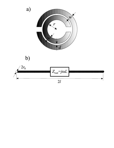
Figure 2: Geometries of resonant scatterers: a) Split-Ring-Resonator, b) inductively loaded wire dipole.

The inverse values of the polarizabilities $\alpha(\omega)$ and $\alpha_{e}(\omega)$ (see Appendix A, formulae (22) and (25)) of SRR:s and ILW:s have the same dependencies on frequency within the resonant band:

$${\rm Re}\{\alpha^{-1}(\omega)\}=A^{-1}\left(\frac{\omega_{0}^{2}}{\omega^{2}}-1\right).$$ (1)

Here $A$ is amplitude and $\omega_{0}$ is resonant frequency, the parameters determined by the geometry of the scatterer. Notice, that the result (1) is also valid for a silver nanosphere in the vicinity of its plasmon resonance Weber and Ford (2004). Thus, it is clear that there is no principal difference between the dispersion properties of the chain of SRR:s and ILW:s (at microwaves) or silver nanospheres (in the optical range).

II Chains of uniaxial resonant scatterers

Let us study dispersion properties of the linear chains with period $a$ formed by resonant scatterers. We will consider only two typical orientations of scatterers: longitudinal and transverse. The geometries of the structures are presented in Fig. 3. The case of longitudinal orientation was analyzed in Tretyakov and Viitanen (2000), and the both longitudinal and transverse orientations were studied in Weber and Ford (2004). In the present section we reproduce the main results of these works with help of the local field approach.

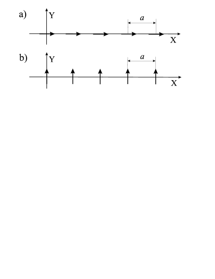
Figure 3: Chains of resonant scatterers. a) Longitudinal orientation. b) Transverse orientation.

II.1 Basic theory

Without loss of generality we can restrict consideration by the case of the chain of magnetic scatterers (SRR:s). The chains of electric scatterers are dual structures to the considered ones and have completely the same dispersion properties.

The spatial distribution of dipole moments of SRR:s corresponding to an eigenmode of a chain is determined by a propagation constant $q$: $M_{n}=Me^{-jqan}$. Following to the local field approach the dipole moment $M$ of a reference (zeroth) scatterer can be expressed in terms of the magnetic field ${\bf H}_{\rm loc.}$ acting to it: $M=\alpha H^{d}_{\rm loc.}$, where $H^{d}_{\rm loc.}=({\bf H}_{\rm loc.}\cdot{\bf d})$ is the projection of the field on the direction of the scatterer (${\bf d}={\bf x}_{0}$ for longitudinal orientation of scatterers and ${\bf d}={\bf y}_{0}$ for transverse one). This local field is a sum of partial magnetic fields ${\bf H}_{m}$ produced at the coordinate origin by all other scatterers with indexes $m\neq 0$: ${\bf H}_{\rm loc.}=\sum\limits_{m\neq 0}{\bf H}_{m}$.

The magnetic field produced by a single scatterer with dipole moment ${\bf M}_{m}$ at a point with radius vector ${\bf R}$ is given by dyadic Green’s function $\overline{\overline{G}}({\bf R})$:

$${\bf H}_{m}({\bf R})=\mu_{0}^{-1}\overline{\overline{G}}({\bf R}){\bf M}_{m},$$ (2)

where

$$\overline{\overline{G}}({\bf R})=\left(k^{2}\overline{\overline{I}}+\nabla\nabla\right)\frac{e^{-jkR}}{4\pi R}.$$ (3)

Since all dipole moments of the chain are oriented along ${\bf d}$ it is enough to use only the ${\bf d}{\bf d}$ component of dyadic Green’s function. So, we replace (2) by the scalar expression:

$$H_{m}^{d}({\bf R})=\mu_{0}^{-1}G_{dd}({\bf R})M_{m},$$ (4)

where

$$G_{dd}({\bf R})=\left(k^{2}+\frac{\partial^{2}}{\partial d^{2}}\right)\frac{e^{-jkR}}{4\pi R},$$ (5)

and $d$ means $x$ for the longitudinal case and $y$ for the transverse case.

Finally we obtain the expression for the field acting to the reference scatterer in the form:

$$H^{d}_{\rm loc.}=\sum\limits_{m\neq 0}G_{dd}(am{\bf x}_{0})e^{-jqam}M.$$ (6)

It allows to get dispersion equation for the chains under consideration:

$$\mu_{0}\alpha(\omega)^{-1}=C_{d}(\omega,q,a),$$ (7)

where

$$C_{d}(\omega,q,a)=\sum\limits_{m\neq 0}G_{dd}(am{\bf x}_{0})e^{-jqam}.$$

In the Appendix B we provide expressions (27) and (28) which we use for effective numerical calculations of interaction constants $C_{x}$ and $C_{y}$, corresponding to transverse and longitudinal orientations of scatterers, respectively.

II.2 Analysis of dispersion properties

The dispersion diagram for guided modes can be obtained solving transcendental dispersion equation (7) with interaction constants given by expressions (27) and (28). Geometrically, dispersion curves correspond to the lines of level where the surface plot of function ${\rm Re}\{C_{x,y}(\omega,q)\}$ is crossed by $\mu_{0}{\rm Re}\{\alpha^{-1}(\omega)\}$. Note, that only the solutions with $k<q<2\pi/a-k$ for $k<\pi/a$ correspond to guided modes: For $|q|<k$, ${\rm Im}\{C_{x,y}(\omega,q)-\mu_{0}\alpha^{-1}\}\neq 0$ and dispersion equation (7) has complex solutions corresponding to leaky modes (see details in Appendix B).

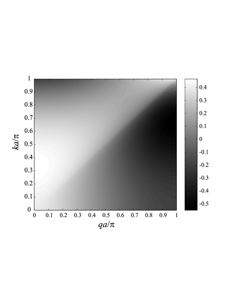
Figure 4: Dependence of ${\rm Re}\{C_{x}a^{3}\}$ on normalized frequency $ka/\pi$ and propagation factor $qa/\pi$

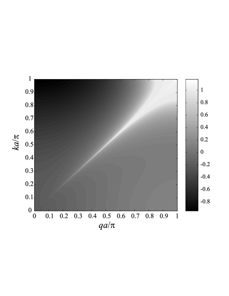
Figure 5: Dependence of ${\rm Re}\{C_{y}a^{3}\}$ on normalized frequency $ka/\pi$ and propagation factor $qa/\pi$

The dependencies of $C_{x}$ and $C_{y}$ on on normalized frequency $ka/\pi$ and propagation factor $qa/\pi$ are shown in Fig. 4 and 5, respectively. The interaction constants vary in $[-1,1]$ range except the case of $C_{y}$ with $q$ close to $k$, which has logarithmic singularity at the light line $q=k$. The function $\mu_{0}{\rm Re}\{\alpha^{-1}(\omega)\}$ decreases very rapidly within $[-1,1]$ range of values near the resonant frequency $\omega_{0}$. It means, that guided modes exist only within a narrow bands near the resonant frequency of scatterers. The behavior of dispersion curves can be easily predicted from the plots in Fig. 4 and 5. If at a fixed frequency the interaction constant decays when propagation factor increases then the dispersion curve grows and the eigenmode is forward wave (the group velocity $v_{g}=\frac{d\omega}{dq}$ is positive), but if the interaction constant grows then the dispersion curve decays and the eigenmode is backward wave (the group velocity $v_{g}=\frac{d\omega}{dq}$ is negative). From Fig. 4 it is clear that for any resonant frequencies satisfying to the evident condition $\omega_{0}<\pi/(a\sqrt{\varepsilon_{0}\mu_{0}})$ (corresponding to the propagation below cutoff of the hollow waveguide ) the longitudinal mode is forward wave because $C_{x}$ decays versus $q$. In the case of transverse modes the situation is different. While $k_{0}a<0.5\pi$ ($k_{0}=\omega_{0}\sqrt{\varepsilon_{0}\mu_{0}}$) a two mode regime holds. The interaction constant $C_{y}$ decays while $q$ is close to $k$, but from a certain $q$ it starts to grow. It means that one of the transverse eigenmodes is forward (with $q\approx k$) and the other one is backward. If the resonant frequency is high enough ($0.5\pi<k_{0}a<\pi$) the two mode regime disappears and only the forward wave remains.

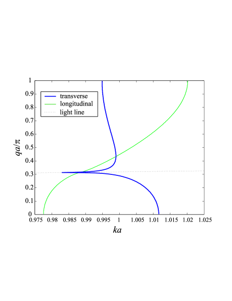
Figure 6: Dispersion diagram for chains of resonant scatterers: transverse (thick line) and longitudinal (thin line) orientations

The typical dispersion diagram for both longitudinal and transverse modes is presented in Fig. 6 for the case of scatterers with $A=0.1\mu_{0}a^{3}$ and $\omega_{0}a=1/\sqrt{\varepsilon_{0}\mu_{0}}$. The similar dispersion diagram was obtained in Weber and Ford (2004) (see Fig. 3 of this work) by a numerical simulation. Though in Weber and Ford (2004) the electric scatterers in the optical range were considered, but we consider the magnetic scatterers in the microwave range, the use of duality principle, and normalized frequency $ka/\pi$ and wave vector $qa/\pi$ eliminates this difference. The polarizability of silver nanospheres, for which Fig. 3 from Weber and Ford (2004) was obtained, obeys to expression (8) of Weber and Ford (2004) which is identical to our formula (1)).

As it was predicted, the longitudinal mode is forward wave and there is a two mode regime for transverse modes. The dispersion curve for transverse waves has the asymptote $q=k$ and both leaky ($q<k$) and guided ($q>k$) modes exist at very low frequencies where they have almost equal wave vectors. This fact indicates the good matching between the radiated wave and the guided mode. Within the band $0.995<ka<1$ there are two guiding modes at every frequency. The solution corresponding to the backward wave is close to the Bragg’s mode ($qa\approx\pi$) whose group velocity is close to zero. The field of this mode is concentrated near the chain within the spatial region $r=\sqrt{z^{2}+y^{2}}<1/\sqrt{q^{2}-k^{2}}\sim a$. The same concerns the longitudinal mode within the band $1.015<ka<1.020$. If the period of the chain is much smaller than wavelength in free space the waveguide is sub-wavelength (the field of the guided mode is concentrated within a cylindrical domain whose diameter is much smaller than $\lambda$). Thus, the chains of resonant scatterers (electric or magnetic, it does not matter) form sub-wavelength waveguides which can support either forward or backward waves Brongersma et al. (2000); Maier et al. (2003, 2002); Weber and Ford (2004); Tretyakov and Viitanen (2000); Shamonina et al. (2002a, b); Wiltshire et al. (2003); E.Shamonina1 and L.Solymar (2004).

III Loaded waveguides

III.1 Basic theory

Let us study the eigenmodes of the rectangular metallic waveguides periodically loaded by resonant uniaxial scatterers. Such structures can be effectively considered as linear chains located inside of the metallic waveguides. The geometries of the four waveguides considered in the present paper are shown in Fig. 1 (left sides of subplots). The chains with period $c$ along the waveguide axis are located at the center of rectangular metallic waveguides with dimensions $a\times b$. The structures in Figs. 1.a-d differ by orientation of scatterers (longitudinal or transverse) and their type (electric or magnetic). The first structure (with transversely oriented magnetic scatterers) is the sub-wavelength waveguide (see Fig. 1) suggested by R. Marques Marques et al. (2002a); Hrabar et al. (2005). The other ones are considered in order to show three other possible ways to obtain miniaturization of rectangular waveguides.

Note, that the chains of electric scatterers are no more dual to the chains of magnetic scatterers (in contrast to the chains in free space) due to the different interaction of electric and magnetic dipoles with metallic walls.

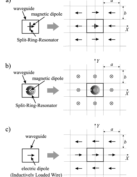
Figure 7: Transformation of the waveguide problem to the lattice one with the use of the image principle

The dispersion equation for the chains keeps the same form as (7), but free-space dyadic Green’s function $\overline{\overline{G}}({\bf R})$ (3) should be replaced by Green’s function of the waveguide which takes into account the metallic walls. This Green’s function can be determined with help of the image principle. This approach transforms the eigenmode problem for the loaded waveguide to the problem of the eigenwave propagation in a three-dimensional electromagnetic lattice formed by same scatterers. The details of the transformation are illustrated by Fig. 7 (right parts of all subplots). The electromagnetic crystals obtained in such a way have orthorhombic elementary cell $a\times b\times c$ and their dispersion properties was studied in Belov and Simovski (2005) using local field approach. Thus, we can apply the theory of the electromagnetic interaction in dipole crystals presented in Belov and Simovski (2005) in order to study dispersion properties of waveguides under consideration.

In the coordinate system associated to the axes of the crystal the center of a scatterer with indexes $(m,n,l)$ has coordinates ${\bf R}_{m,n,l}=(am,bn,cl)^{T}$. From Fig. 7 it is clear, that distribution of dipole moments in the lattice has the following form:

$${\bf M}_{m,n,l}=(-1)^{m}Me^{-jqcl}{\bf x}_{0},$$

for the case of transverse orientation of magnetic scatterers (Fig. 7.a);

$${\bf M}_{m,n,l}=Me^{-jqcl}{\bf z}_{0},$$

for the case of longitudinal orientation of magnetic scatterers (Fig. 7.b);

$${\bf P}_{m,n,l}=(-1)^{n}Pe^{-jqcl}{\bf x}_{0},$$

for the case of transverse orientation of electric scatterers (Fig. 7.c); and

$${\bf P}_{m,n,l}=(-1)^{m+n}Pe^{-jqcl}{\bf z}_{0},$$

for the case of longitudinal orientation of electric scatterers (Fig. 7.d).

Any of these distributions can be rewritten in terms of a wavevector ${\bf q}$ as $e^{-j({\bf q}\cdot{\bf R}_{m,n,l})}$, where the wavevector ${\bf q}$ for four cases considered above has the form $(\pi/a,0,q)^{T}$, $(0,0,q)^{T}$, $(0,\pi/b,q)^{T}$ and $(\pi/a,\pi/b,q)^{T}$, respectively. This notation finally makes clear that the waveguide dispersion problems reduce to those of the three-dimensional lattices in the special cases of certain propagation directions.

The dispersion equation for three-dimensional electromagnetic crystal formed by magnetic scatterers oriented along $x$-axis has the form Belov and Simovski (2005):

$$\mu_{0}\alpha^{-1}(\omega)-C(k,{\bf q})=0,$$ (8)

where

$$C(k,{\bf q},a,b,c)=\sum\limits_{(m,n,l)\neq(0,0,0)}G({\bf R}_{m,n,l})e^{-j(q_{x}am+q_{y}bn+q_{z}cl)}.$$ (9)

We call $C(k,{\bf q},a,b,c)$ as the dynamic interaction constant of the lattice using the analogy with the classical interaction constant from the theory of artificial dielectrics and magnetics Collin (1990). The explicit expression for $C$ for the general case was derived in Belov and Simovski (2005) and it is given in Appendix C by formula (37).

The dispersion equation for waveguides with transverse orientation of scatterers can be directly obtained from equation (8) by substitution ${\bf q}=(\pi/a,0,q)^{T}$ and ${\bf q}=(0,\pi/b,q)^{T}$ for magnetic and electric scatterers, respectively. Also, in the case of electric scatterers following duality principle $\mu_{0}\alpha^{-1}(\omega)$ should be replaced by $\varepsilon_{0}\alpha_{e}^{-1}(\omega)$. The similar operation for case of longitudinal orientation happens to be possible only after rotation of coordinate axes: $z\rightarrow x^{\prime}$, $x\rightarrow y^{\prime}$, $y\rightarrow z^{\prime}$, since equation (8) requires scatterers to be directed along $x$-axis, but for longitudinal orientation they are directed along $z$-axis. After such manipulation substitution of ${\bf q}=(q,0,0)^{T}$ and ${\bf q}=(q,\pi/a,\pi/b)^{T}$ (in the new coordinate axes $(x^{\prime},y^{\prime},z^{\prime})$) into equation (8) provide desired dispersion equations for waveguides with transverse orientation of magnetic and electric scatterers, respectively.

This way we obtain the following dispersion equations for all loaded waveguides under consideration:

$$\mu_{0}\alpha^{-1}(\omega)-C(k,(\pi/a,0,q)^{T},a,b,c)=0,$$ (10)

for transverse orientation of magnetic scatterers;

$$\mu_{0}\alpha^{-1}(\omega)-C(k,(q,0,0)^{T},c,a,b)=0,$$ (11)

for longitudinal orientation of magnetic scatterers;

$$\varepsilon_{0}\alpha_{e}^{-1}(\omega)-C(k,(0,\pi/b,q)^{T},a,b,c)=0,$$ (12)

for transverse orientation of electric scatterers; and

$$\varepsilon_{0}\alpha_{e}^{-1}(\omega)-C(k,(q,\pi/a,\pi/b)^{T},c,a,b)=0,$$ (13)

for longitudinal orientation of electric scatterers.

The obtained dispersion equations are real valued ones, because the imaginary parts of its components cancels out. It can be clearly seen from Sipe-Kronendonk condition (23) and following expression proved in Belov and Simovski (2005):

$${\rm Im}(C)=\frac{k^{3}}{6\pi}.$$ (14)

III.2 Effective medium filling approximation

The chain of SRR:s with transverse orientation located in the waveguide has been interpreted in the literature as a piece of an uniaxial magnetic medium Marques et al. (2002a); Hrabar et al. (2005). We call this approach as effective medium filling approximation. It can be applied practically to every waveguide considered in this paper except the case of longitudinal orientation of magnetic scatterers since the uniaxial magnetic model does not describe longitudinal modes. This approach provide qualitatively acceptable results which are compared with exact ones in the next subsection.

Let us start from the case of transversely oriented magnetic scatterers (Fig. 7.a) and consider a chain of parallel uniaxial magnetic scatterers as a piece of infinite resonant uniaxial magnetic. The permeability of such a magnetic is a tensor (dyadic) of the form:

$$\overline{\overline{\mu}}=\mu{\bf x}_{0}{\bf x}_{0}+\mu_{0}({\bf y}_{0}{\bf y}_{0}+{\bf z}_{0}{\bf z}_{0}).$$

The permeability $\mu$ along the anisotropy axis $x$, can be calculated though the individual polarizability of a single scatterer using the Clausius-Mossotti formula:

$$\mu=\mu_{0}\left(1+\frac{\alpha(\omega)/(\mu_{0}V)}{1-C_{s}(a,b,c)\alpha(\omega)/\mu_{0}}\right),$$ (15)

where $V=abc$ is a volume of the elementary cell of an infinite three-dimensional lattice and $C_{s}(a,b,c)$ is the known static interaction constant of the lattice Collin (1990); Belov and Simovski (2005). In the case of a simple cubic lattice $a=b=c$ the interaction constant is equal to the classical value $C_{s}=1/(3V)$.

Notice, that we should skip the radiation losses contribution in expression (24) while substituting into formula (15). This makes permeability purely real number as it should be for lossless material. This manipulation is based on the fact that the far-field radiation of the single scatterer is compensated by the electromagnetic interaction in a regular three-dimensional array, so that there were no radiation losses for the wave propagating in the lattice Sipe and Kranendonk (1974); Belov and Simovski (2005).

The dispersion equation for the uniaxial magnetic medium has the following form (see e.g. Belov (2003)):

$$\mu_{0}(q_{y}^{2}+q_{z}^{2})=\mu(k^{2}-q_{x}^{2}).$$ (16)

To solve the waveguide dispersion problem is to solve the dispersion problem (16) for a special case ${\bf q}=(\pi/a,0,q)^{T}$. The substitution of ${\bf q}=(\pi/a,0,q)^{T}$ into (16) gives:

$$q^{2}=\frac{\mu}{\mu_{0}}\left[k^{2}-\left(\frac{\pi}{a}\right)^{2}\right].$$ (17)

For the frequencies below cutoff of the hollow waveguide the expression in the brackets of (17) is negative and for positive $\mu$ there is no propagation. However, if $\mu$ is negative (it happens in accordance with (22) and (15) within a narrow frequency range near the resonance of the scatterers, just above the resonant frequency of the media) $q$ becomes real. This mini pass-band can be located much lower than the cutoff frequency of the empty waveguide with help of reduction of resonant frequency of the scatterers. It is easy to see from (17) that the mode is backward wave, i.e. $\frac{dq}{d\omega}<0$. This follows from the basic inequality $\frac{d\mu}{d\omega}>0$ (Foster’s theorem).

So, for transverse magnetic scatterers the effective medium filling model gives (at least qualitatively) a correct result. Namely, it predicts a mini-band within the resonance band of SRRs and the backward wave propagating within it. However, this model is not accurate. The reason of this inaccuracy is simple. In spite of the low frequency of operation (the waveguide dimensions are small compared to the wavelength in free space) the effective magnetic medium should operate in the regime when its period is comparable with the wavelength in the effective medium because $q_{x}=\pi/a$. Such regime for an electromagnetic crystal can not be described with help of homogenization and requires taking into account spatial resonances of the lattice Belov and Simovski (2005).

In the case of transversely oriented electric scatterers (Fig. 7.c) the effective medium filling model implies that the wave propagates in a uniaxial dielectric with permittivity tensor:

$$\overline{\overline{\varepsilon}}=\mu{\bf x}_{0}{\bf x}_{0}+\varepsilon_{0}({\bf y}_{0}{\bf y}_{0}+{\bf z}_{0}{\bf z}_{0}).$$

The permittivity $\varepsilon$ along the anisotropy axis $x$ is given by the Clausius-Mossotti formula:

$$\varepsilon=\varepsilon_{0}\left(1+\frac{\alpha_{e}(\omega)/(\varepsilon_{0}V)}{1-C_{s}(a,b,c)\alpha_{e}(\omega)/\varepsilon_{0}}\right).$$ (18)

The dispersion equation for such uniaxial dielectric reads Belov (2003):

$$\varepsilon_{0}(q_{y}^{2}+q_{z}^{2})=\varepsilon(k^{2}-q_{x}^{2}).$$ (19)

Solution of waveguide dispersion problem corresponds to the case when ${\bf q}=(0,\pi/b,q)^{T}$:

$$q^{2}=\frac{\varepsilon}{\varepsilon_{0}}k^{2}-\left(\frac{\pi}{b}\right)^{2}.$$ (20)

This mode propagates only at the frequencies when permittivity takes high positive values $\varepsilon>\varepsilon_{0}[\pi/(kb)]^{2}$. In our case of resonant dielectric it happens within a mini-band just below the resonance of the medium. It is clear from (20) that the mode is forward wave, i.e. $\frac{dq}{d\omega}>0$. This follows from the Foster’s theorem $\frac{d\varepsilon}{d\omega}>0$.

In the case of longitudinally oriented electric scatterers (Fig. 7.d) the solution of the waveguide dispersion problem can be obtained from the dispersion equation (19) with ${\bf q}=(q,\pi/a,\pi/b)^{T}$ (the axis were transformed in order to have x-axis along dipoles) in the next form:

$$q^{2}=k^{2}-\frac{\varepsilon_{0}}{\varepsilon}\left[\left(\frac{\pi}{a}\right)^{2}+\left(\frac{\pi}{b}\right)^{2}\right].$$ (21)

The mode is propagating at the frequencies when permittivity is positive and rather high, or negative. This mode is forward wave in the same manner as (20) since $\frac{d\varepsilon}{d\omega}>0$.

III.3 Analysis of dispersion properties

For numerical calculation of dispersion curves using (10), (11), (12), (13) and (37) we have chosen square waveguides ($a=b=c$) loaded by scatterers with the same parameters which were used for studies of chains: $\omega_{0}=1/(a\sqrt{\varepsilon_{0}\mu_{0}})$, and $A=0.1\mu_{0}a^{3}$ for magnetic scatterers, and $A_{e}=0.1\epsilon_{0}a^{3}$ for electric ones.

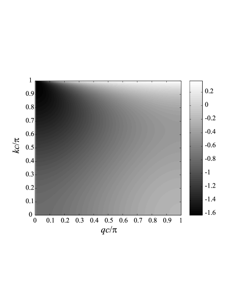
Figure 8: Dependence of the real part of normalized interaction constant $C(k,{\bf q})a^{3}$ with ${\bf q}=(\pi/a,0,q)^{T}$ (corresponding to transverse orientation of magnetic scatterers) on normalized frequency $ka/\pi$ and propagation constant $qa/\pi$.

The dependence of the real part of normalized interaction constant $C(k,{\bf q})$ with ${\bf q}=(\pi/a,0,q)^{T}$ on the normalized frequency $ka/\pi$ and on the propagation constant $qa/\pi$ is presented in Fig. 8. This interaction constant corresponds to dispersion equation (10) for transverse orientation of magnetic scatterers. The value of $\mbox{Re}(C)a^{3}$ varies within $[-2,0.5]$ interval while the normalized frequency $ka/\pi$ is bounded by unity (which corresponds to the cutoff of hollow waveguide). If a value of the normalized frequency is fixed then the real part of the interaction constant is a monotonously growing function of $qa/\pi$. The dependence of the real part of the interaction constant on frequency is quite weak as compared with rapidly decreasing $\alpha^{-1}(\omega)$ as follows from (24). The function $\mu_{0}\alpha^{-1}(\omega)$ takes values within $[-2,0.5]$ interval at the frequencies close to resonant frequency $\omega_{0}$. Therefore, dispersion equation (10) has a real solution for $qa/\pi$ within a mini-band of frequencies near the resonant frequency of the scatterers $\omega_{0}$, and this solution is a decaying function of frequency which corresponds to the backward wave (the group velocity $v_{g}=\frac{d\omega}{dq}$ is negative). The obtained result, of course, confirms existence of backward wave below cutoff of the hollow waveguide predicted and experimentally demonstrated in Marques et al. (2002a); Hrabar et al. (2005).

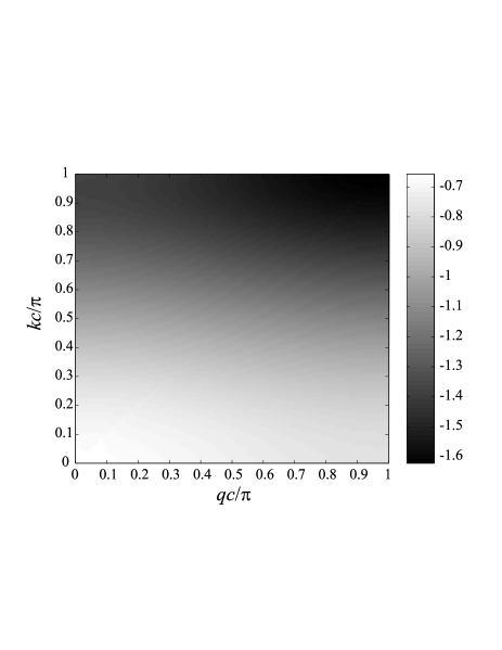
Figure 9: Dependence of the real part of normalized interaction constant $C(k,{\bf q})a^{3}$ with ${\bf q}=(q,0,0)^{T}$ (corresponding to longitudinal orientation of magnetic scatterers) on normalized frequency $ka/\pi$ and propagation constant $qa/\pi$.

In contrast to Fig. 8, the dependencies of normalized interaction constants $C(k,{\bf q})$ with ${\bf q}=(q,0,0)^{T}$, ${\bf q}=(0,\pi/a,q)^{T}$ and ${\bf q}=(q,\pi/a,\pi/a)^{T}$ are decaying functions of $q$ for the fixed values of $k<\pi/a$. It means that solutions of dispersion equations (11), (12) and (13) are forward waves for any resonant frequency of the scatterer below $\pi/(a\sqrt{\varepsilon_{0}\mu_{0}})$. The Fig. 9 shows dependence of the real part of normalized interaction constant $C(k,{\bf q})$ with ${\bf q}=(q,0,0)^{T}$ on the normalized frequency $ka/\pi$ and on the propagation constant $qa/\pi$. The dependencies for the cases ${\bf q}=(0,\pi/a,q)^{T}$ and ${\bf q}=(q,\pi/a,\pi/a)^{T}$ are not shown in order to reduce size of the paper.

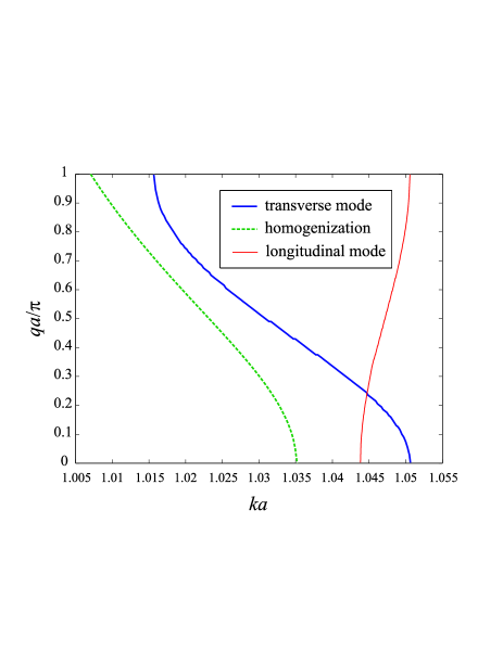
Figure 10: Dispersion curves for metallic waveguides loaded by magnetic scatterers: exact solution (thick line) and effective medium filling approximation (dashed line) for transverse orientation, and exact solution (thin line) for longitudinal orientation. The effective medium filling model for the longitudinal case is not applicable.

The dispersion curves for the case of magnetic scatterers are presented in Fig. 10. The thick solid line represents the dispersion curve for the transverse mode. It is obtained by numerical solution of transcendental dispersion equation (10). The dashed line shows the result predicted by the model of effective medium filling (17). The significant frequency shift between the exact and approximate solutions is observed. Also, the effective medium model gives wittingly wrong results with $q>\pi/a$ in the region $ka<1.0055$, and incorrectly describes group velocity for $q>\pi/(2a)$ (for example, it does not describe the Bragg mode with zero group velocity at the point $qa=\pi$). The dispersion curve for the longitudinal mode obtained by numerical solution of equation (11) is represented by thin line in Fig. 10. As it was mentioned above, the effective medium filling model can not be applied for description of this mode.

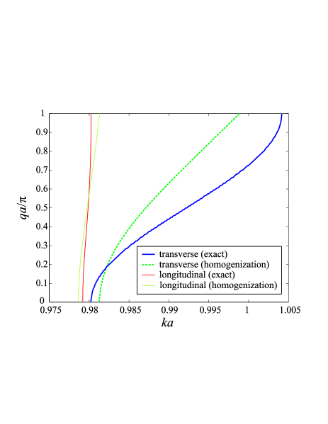
Figure 11: Dispersion curves for metallic waveguides loaded by electric scatterers: exact solution (thick line) and effective medium filling approximation (dashed line) for transverse orientation, and exact solution (thin line) and effective medium filling approximation (thin dashed line) for longitudinal orientation.

The dispersion curves for the case of electric scatterers are presented in Fig. 11. The thick and thin solid lines shows dispersion curves for transverse and longitudinal modes, obtained by numerical solution of dispersion equations (12) and (13), respectively. The dispersion curves provided by effective medium models for transverse and longitudinal modes (formulae (20) and (21)) are plotted by thick and thin dashed lines, respectively. The comparison of exact and approximate solutions shows that the model of effective medium filling gives qualitatively right prediction of dispersion curves behavior in the case of electric scatterers as well as in the case of transverse magnetic scatterers. The drawbacks are also the same: wrong group velocity $q>\pi/(2a)$ and wittingly wrong results with $q>\pi/a$ at some frequencies.

The Figs. 10 and 11 demonstrate that the waveguides loaded by electric and magnetic resonant scatterers support modes within the mini-bands below the cutoff frequency of the hollow waveguide. The modes are forward waves, except the case of transverse magnetic scatterers when the mode is forward wave. The bandwidth in the case of transverse electric scatterers is of the same order with bandwidth for magnetic scatterers with the same parameters obtained with help of duality principle, but the bandwidths for the longitudinal modes are significantly narrower than for the transverse ones.

IV Discussion

In the papers Marques et al. (2002a); Hrabar et al. (2005) the term ‘subwavelength waveguide’ was applied to a rectangular waveguide with small transversal dimensions as compared to the wavelength in free space. However, there is a lot of other works Brongersma et al. (2000); Maier et al. (2003, 2002); Weber and Ford (2004); Tretyakov and Viitanen (2000); Shamonina et al. (2002a, b); Wiltshire et al. (2003); E.Shamonina1 and L.Solymar (2004). in which the term ‘subwavelength waveguiding’ means the propagation of a wave along the chain of electrically small nearly-resonant particles below the diffraction limit. In this case the transversal size of the spatial domain, in which the field of the guided mode is concentrated, is much smaller that the wavelength in free space. Therefore, this mechanism of the wave transmission is considered as prospective for subwavelength imaging.

Since the field of the mode guided along the chain of resonant scatterers is concentrated within a subwavelength cross section, the presence of the metal walls even at the rather small distance turns out to be not crucial for the existence of the guided wave. Thus, any waveguide periodically loaded by the scatterers can be considered as a subwavelength waveguide formed by the chain of nearly resonant scatterers, whose dispersive properties are perturbed by the metal walls. These walls can be described in terms of the image chains forming an infinite lattice. However, the wave propagates along the same direction in every image chain, and the transversal wave numbers $q_{x}=\pi/a$ or $q_{y}=\pi/b$ describe the transversal phase distribution of the wave propagating along $z$ but not the energy transport across $z$. The main question is how the image chains of scatterers interact with the real chain, and how this interaction influences its dispersive properties.

For that purpose let us compare Fig. 6 with Figs. 10 and 11. We can conclude that the presence of metal walls around the chain of resonant scatterers produces the following effects:

• It decreases the group velocity and the frequency band of the guided mode which corresponds to the longitudinal orientation of dipoles.

• It cancels the two-mode regime for the transverse orientation of dipoles, so that the dispersion branch becomes backward for magnetic scatterers, and forward for electric ones.

Finally, we would like to emphasize, that the width of the pass band for the waveguide loaded by transversal electric scatterers has the same order as in the case of transversal magnetic scatterers (Marques waveguide Marques et al. (2002a); Hrabar et al. (2005)) if the loading scatterers have parameters obtained using duality principle from each other. So, the loading by electric scatterers could be an alternative and even more appropriate solution for the waveguide miniaturization than the design suggested in Hrabar et al. (2005) for this purpose.

V Conclusion

The dispersion properties of rectangular waveguides loaded by resonant scatterers (magnetic and electric ones) have been studied. The waveguide problem has been transformed using the image theory into the eigenmode problem of an auxiliary three-dimensional electromagnetic crystal. The dispersion properties of such electromagnetic crystal have been modelled using the local field approach. It has been revealed that not only magnetic but also electric resonant scatterers allow to obtain mini pass band below cutoff frequency of the hollow waveguide. The corresponding mini-band turns out to be of the same order as for magnetic scatterers with same individual frequency dispersion. So, the electric scatterers (inductively loaded short wires) could be also prospective for the waveguide miniaturization as well as split-ring-resonators. It has been shown that the loading by scatterers with longitudinal orientation of dipole moments also allows to obtain the mini-band of propagation below the cutoff frequency of the hollow waveguide, but the width of this band is significnatly narrower as compared to the case of transverse orientation. The observed effects are explained in terms of the subwavelength guiding properties of the single chains of scatterers. This explanation is supported by comparison of dispersion properties of the loaded waveguides and the chains of the resonant scatterers in free space. Results of our theory are in good agreement with the known literature data. For the chains of resonant dipoles the results from Weber and Ford (2004) are reproduced. For the rectangular waveguide loaded by split-ring-resonators the same result as in Marques et al. (2002a) has been obtained.

Appendix A Polarizabilities of resonant scatterers

A.1 Split-Ring Resonators

The SRR considered in Pendry et al. (1999); Smith et al. (2000); Shelby et al. (2001) is a pair of two coplanar broken metal rings (see Fig.2.b). Since the two loops of an SRR are not identical the analytical models of it are rather cumbersome Marques et al. (2002b); Sauviac et al. (2004). In fact, such SRR can not be described as a purely magnetic scatterer, because it exhibits bianisotropic properties and has resonant electric polarizability Marques et al. (2002b); Sauviac et al. (2004) (see also discussion in Simovski et al. (2003)). However, the electric polarizability and bianisotropy of SRR is out of the scope of this paper. We neglect these effects and consider an ordinary SRR as a magnetic scatterer. The analytical expressions for the magnetic polarizability $\alpha(\omega)$ of SRRs with geometry plotted in Fig.2.a were derived and validated in Sauviac et al. (2004). The final result reads as follows:

$$\alpha(\omega)=\frac{A\omega^{2}}{\omega_{0}^{2}-\omega^{2}+j\omega\Gamma},\qquad A=\frac{\mu_{0}^{2}\pi^{2}r^{4}}{L+M},$$ (22)

where $\omega_{0}$ is the resonant frequency of magnetic polarizability:

$$\omega_{0}^{2}=\frac{1}{(L+M)C_{r}},$$

$L$ is inductance of the ring (we assume that both rings have the same inductance):

$$L=\mu_{0}r\left[\log\left(\frac{32R}{w}\right)-2\right],$$

$M$ is mutual inductance of the two rings:

$$M=\mu_{0}r\left[(1-\xi)\log\left(\frac{4}{\xi}\right)-2+\xi\right],\qquad\xi=\frac{w+d}{2r},$$

$C_{r}$ is the effective capacitance of the SRR:

$$C_{r}=\varepsilon_{0}\frac{r}{\pi}{\rm arccosh}\left(\frac{2w}{d}\right),$$

$\Gamma$ is the radiation reaction factor:

$$\Gamma=\frac{A\omega k^{3}}{6\pi\mu_{0}},$$

$r$ is the inner radius of the inner ring, $w$ is the width of the rings, $d$ is distance between the edges of the rings (see Fig.2.a), $\varepsilon_{0}$ and $\mu_{0}$ are permittivity and permeability of the host media, and $k=\omega\sqrt{\varepsilon_{0}\mu_{0}}$ is the wave number of the host medium. The presented formulae are valid within the frame of the following approximations: $w,d\ll r$ and the splits of the rings are large enough compared to $d$. Also, we assume that SRR is formed by ideally conducting rings (no dissipation losses).

The magnetic polarizability (22) takes into account the radiation losses and satisfies to the basic Sipe-Kranendonk condition Sipe and Kranendonk (1974); Belov et al. (2003, 2002) which in the present case has the following form:

$${\rm Im}\left\{\alpha^{-1}(\omega)\right\}=\frac{k^{3}}{6\pi\mu_{0}}.$$ (23)

In our analysis we operate with the inverse polarizability $\alpha^{-1}(\omega)$, thus, we rewrite (22) in the following form:

$$\alpha^{-1}(\omega)=A^{-1}\left(\frac{\omega_{0}^{2}}{\omega^{2}}-1\right)+j\frac{k^{3}}{6\pi\mu_{0}}.$$ (24)

A.2 Inductively Loaded Short Wires

An inductively loaded short wire is shown in Fig. 2.b. The electric polarizability $\alpha_{e}$ of an inductively loaded wire following the known model Tretyakov et al. (2003) has the form:

$$\alpha_{e}^{-1}=\frac{3}{l^{2}C_{\rm wire}}\left(\frac{1-\omega^{2}/\omega_{0}^{2}}{4-\omega^{2}/\omega_{0}^{2}}\right)+j\frac{k^{3}}{6\pi\varepsilon_{0}}$$ (25)

where $C_{\mbox{wire}}=\pi l\varepsilon_{0}/\log(2l/r_{0})$ is the capacitance of the wire, $\omega_{0}=\sqrt{LC_{\rm wire}}$ is the resonant frequency, $L$ is the inductance of the load, $l$ is the half length of the wire and $r_{0}$ is the wire radius.

It is clear, that at the frequencies near the resonance the polarizability of LSW has the form

$$\alpha_{e}^{-1}(\omega)\approx A_{e}^{-1}\left(\frac{\omega_{0}^{2}}{\omega^{2}}-1\right)+j\frac{k^{3}}{6\pi\varepsilon_{0}},$$ (26)

with $A_{e}=l^{2}C_{\rm wire}$, which is similar to (24). Moreover, if $A_{e}/\varepsilon_{0}=A/\mu_{0}$ then using duality principle the magnetic dipole with polarizability $\alpha$ (24) can be transformed to the electric dipole with polarizability $\alpha_{e}$ (24), and vice versa. This means that it is enough to consider only one type of resonant scatterers. In the present paper we have chosen magnetic ones to be principal. The case of electric scatterers was obtained using the duality principle with $A=\mu_{0}A_{e}/\varepsilon_{0}$.

Appendix B Interaction constants of the chains

The initial expressions for the interaction constants $C_{x,y}$ entering (7) follow from (4) and (5) and read as follows:

$$C_{x}=\sum\limits_{m\neq 0}\frac{1+jka|m|}{2\pi a^{3}|m|^{3}}e^{-j(k|m|+qm)a}$$ (27)

$$=\frac{1}{\pi a^{3}}\sum\limits_{m=1}^{+\infty}\left[\frac{1}{m^{3}}+\frac{jka}{m^{2}}\right]e^{-jkam}\cos(qam),$$

for the longitudinal polarization, and

$$C_{y}=\sum\limits_{m\neq 0}\frac{k^{2}a^{2}m^{2}-jka|m|-1}{4\pi a^{3}|m|^{3}}e^{-j(k|m|+qm)a}$$ (28)

$$=\frac{1}{2\pi a^{3}}\sum\limits_{m=1}^{+\infty}\left[\frac{k^{2}a^{2}}{m}-\frac{jka}{m^{2}}-\frac{1}{m^{3}}\right]e^{-jkam}\cos(qam)$$

for the transverse one (see e.g. Weber and Ford (2004)).

Note, that $C_{x}$ includes only near-field terms (of the order $1/R^{2}$ and $1/R^{3}$). In contrast to $C_{x}$, the transverse interaction constant $C_{y}$ includes also the wave terms (of the order $1/R$) which corresponds to the slowly converging series. It makes the direct numerical summation of (28) to be not efficient. The series in (27) have better convergence, but it is also not enough for rapid calculations.

The application of acceleration technique done in Belov and Simovski (2005) offers a more cumbersome expression for $C_{x}(k,q,a)$ than (27), but it is better for numerical calculations since the series converges very rapidly:

$$C_{x}=\frac{1}{4\pi a^{3}}\left[4\sum\limits_{m=1}^{+\infty}\frac{(2jka+3)m+2}{m^{3}(m+1)(m+2)}e^{-jkam}\cos(qam)\right.$$

$$-(jka+1)\left(t_{+}^{2}\log t^{+}+t_{-}^{2}\log t^{-}+2e^{jka}\cos(qa)\right)$$ (29)

$$\left.-2jka\left(t_{+}\log t^{+}+t_{-}\log t^{-}\right)+(7jka+3)\vphantom{\sum\limits_{m=1}^{+\infty}\frac{(2jka+3)m+2}{m^{3}(m+1)(m+2)}}\right],$$

where

$$t^{+}=1-e^{-j(k+q)a},\qquad t^{-}=1-e^{-j(k-q)a},$$

$$t_{+}=1-e^{j(k+q)a},\qquad t_{-}=1-e^{j(k-q)a}.$$

As to $C_{y}$, the series of the order $1/m$ in (28) can be obtained in the closed form using the tabulated formula (see Collin (1990), Appendix):

$$\sum\limits_{m=1}^{+\infty}\frac{e^{-j\gamma m}}{m}=-\log\left(1-e^{-j\gamma}\right)$$ (30)

$$=-\left(\log\left|2\sin\frac{s}{2}\right|+j\frac{\pi-\gamma^{\prime}}{2}\right),$$

where $\gamma^{\prime}=2\pi\{\gamma/(2\pi)\}$ and we use notation $\{x\}$ for fractional part of variable $x$. The rest part of the expression (28) is simply proportional to $C_{x}$. Thus, $C_{y}$ can be evaluated as follows:

$$C_{y}(k,q,a)=-\frac{k^{2}}{4\pi a}\log\left|2\left(\cos ka-\cos qa\right)\right|$$

$$-j\frac{k^{2}}{4a}\left(1-\left\{\frac{(k+q)a}{2\pi}\right\}-\left\{\frac{(k-q)a}{2\pi}\right\}\right)-C_{x}(k,q,a)/2.$$ (31)

In the works Belov and Simovski (2005); Tretyakov and Viitanen (2000) it was shown that

$${\rm Im}(C_{x})=\frac{k^{3}}{6\pi}+\frac{1}{4a}\sum\limits_{|q_{m}|<k}\left(q_{m}^{2}-k^{2}\right),$$ (32)

where

$$q_{m}=q+\frac{2\pi m}{a}.$$

From the formula (28) using some algebra it follows that

$${\rm Im}(C_{y})=\frac{k^{3}}{6\pi}-\frac{1}{8a}\sum\limits_{|q_{m}|<k}\left(q_{m}^{2}+k^{2}\right).$$ (33)

The expressions (32) and (33) demonstrate energy transformations happening in the chains. A single scatterer radiates cylindrical wave and that is why its polarizability has radiation losses which can be described by Sipe-Kronendonk condition (23). Being arranged into the regular chains the scatterers acquire effective polarizability (with respect to the external field) of the form:

$$\alpha_{x,y}=\left[\alpha^{-1}-\mu_{0}^{-1}C_{x,y}\right]^{-1},$$ (34)

where indices $x$ and $y$ correspond to longitudinal and transverse orientations of scatterers in the chain, respectively. In accordance to (32) and (33) one can formulate the following analogues of Sipe-Kronendonk condition for effective polarizabilities of the scatterers in the chains:

$${\rm Im}\left\{\alpha_{x}^{-1}\right\}=\frac{1}{4\mu_{0}a}\sum\limits_{|q_{m}|<k}\left(k^{2}-q_{m}^{2}\right),$$ (35)

$${\rm Im}\left\{\alpha_{y}^{-1}\right\}=\frac{1}{8\mu_{0}a}\sum\limits_{|q_{m}|<k}\left(q_{m}^{2}+k^{2}\right).$$ (36)

Note, that terms $k^{3}/(6\pi)$ are canceled. It is clear, that if there are no such index $m$ that $|q_{m}|<k$ (like it happens for example if $k<q<2\pi/a-k$ for $k<\pi/a$) then effective polarizabilities turn out to be purely real and the chain itself does not radiate. This regime corresponds to the case of guiding modes and it makes dispersion equation (7) real valued one. If there are some indices $m$ that $|q_{m}|<k$ then the effective polarizabilites acquire non-zero imaginary part which give evidence that the chain radiates cylindrical waves. The number of such waves corresponds to the number of indices $m$ fulfilling to the relation $|q_{m}|<k$. If $|q|<k<\pi/a$ then the chain radiates only one cylindrical wave which can be treated as the main diffraction lobe of this periodical array. For the higher frequencies the grating lobes appears and all of them make its contribution to expressions (35) and (36).

Appendix C Interaction constant of an orthorhombic lattice

For effective numerical calculation of interaction constant $C(k,{\bf q},a,b,c)$ defined by (9) we use the following formula deducted in Belov and Simovski (2005):

$$C(k,{\bf q},a,b,c)=-\sum\limits_{n=1}^{+\infty}\sum\limits_{{\rm Re}(p_{m})\neq 0}\frac{p_{m}^{2}}{\pi a}K_{0}\left(p_{m}bn\right)\cos(q_{y}bn)$$

$$+\sum\limits_{m=-\infty}^{+\infty}\sum\limits_{n=-\infty}^{+\infty}\frac{p_{m}^{2}}{2jabk_{z}^{(mn)}}\frac{e^{-jk_{z}^{(mn)}c}-\cos q_{z}c}{\cos k_{z}^{(mn)}c-\cos q_{z}c}$$ (37)

$$-\sum\limits_{{\rm Re}(p_{m})=0}\frac{p_{m}^{2}}{2ab}\left(\frac{1}{jk_{z}^{(m0)}}+\sum\limits_{n=1}^{+\infty}\left[\frac{1}{jk_{z}^{(m,n)}}+\frac{1}{jk_{z}^{(m,-n)}}\right.\right.$$

$$\left.\left.-\frac{b}{\pi n}-\frac{l_{m}b^{3}}{8\pi^{3}n^{3}}\right]+1.202\frac{l_{m}b^{3}}{8\pi^{3}}+\frac{b}{\pi}\left(\log\frac{b|p_{m}|}{4\pi}+\gamma\right)+j\frac{b}{2}\vphantom{\sum\limits_{n\neq 0}\left[\frac{1}{jk_{z}^{(mn)}}-\frac{b}{2\pi|n|}\right]}\right)$$

$$+C_{x}(k,q_{x},a),$$

where $C_{x}$ is given by (29) and

$$k_{x}^{(m)}=q_{x}+\frac{2\pi m}{a},\qquad k_{y}^{(n)}=q_{y}+\frac{2\pi n}{b},$$

$$p_{m}=\sqrt{\left(k_{x}^{(m)}\right)^{2}-k^{2}},\qquad l_{m}=2q_{y}^{2}-p_{m}^{2},$$

$$k_{z}^{(mn)}=-j\sqrt{\left(k_{x}^{(m)}\right)^{2}+\left(k_{y}^{(n)}\right)^{2}-k^{2}}.$$

References

- Marques et al. (2002a) R. Marques, J. Martel, F. Mesa, and F. Medina, Phys. Rev. Lett. 89, 183901 (2002a).
- Hrabar et al. (2005) S. Hrabar, J. Bartolic, and Z. Sipus, IEEE Trans. Antennas Propagat. 53, 110 (2005).
- Pendry et al. (1999) J. Pendry, A. Holden, D. Robbins, and W. Stewart, IEEE Trans. Microw. Theory Techn. 47, 195 (1999).
- Marques et al. (2002b) R. Marques, F. Medina, and R. Rafii-El-Idrissi, Phys. Rev. B 65, 144440 (2002b).
- Smith et al. (2000) D. R. Smith, W. J. Padilla, D. C. Vier, S. C. Nemat-Nasser, and S. Schultz, Phys. Rev. Lett. 84, 4184 (2000).
- Veselago (1968) V. Veselago, Sov. Phys. Usp. 10, 509 (1968).
- Met (2003) Special issue on Metamaterials of IEEE Trans. Antennas and Propagat. 51 (2003).
- Lindell et al. (2001) I. Lindell, S. Tretyakov, K. Nikoskinen, and S. Ilvonen, Microwave and Optical Technology Letters 31, 129 (2001).
- Brongersma et al. (2000) M. Brongersma, J. Hartman, and H. A. Atwater, Phys. Rev. B 62, 16356 (2000).
- Maier et al. (2003) S. Maier, P. Kik, and H. Atwater, Phys. Rev. B 67, 205402 (2003).
- Maier et al. (2002) S. Maier, M. Brongersma, P. Kik, and H. A. Atwater, Phys. Rev. B 65, 193408 (2002).
- Weber and Ford (2004) W. Weber and G. Ford, Phys. Rev. B 70, 125429 (2004).
- Shamonina et al. (2002a) E. Shamonina, V. A. Kalinin, K. H. Ringhofer, and L. Solymar, Journal of Applied Physics 92, 6252 (2002a).
- Shamonina et al. (2002b) E. Shamonina, V. A. Kalinin, K. H. Ringhofer, and L. Solymar, Electronics Letters 38, 371 (2002b).
- Wiltshire et al. (2003) M. Wiltshire, E. Shamonina, I. Young, and L. Solymar, Electronics Letters 39, 215 (2003).
- E.Shamonina1 and L.Solymar (2004) E.Shamonina1 and L.Solymar, J. Phys. D: Appl. Phys. 37, 362 367 (2004).
- Tretyakov and Viitanen (2000) S. Tretyakov and A. Viitanen, Electrical Engineering 82, 353 (2000).
- Shelby et al. (2001) R. A. Shelby, D. R. Smith, and S. Schultz, Science 292, 77 (2001).
- Tretyakov et al. (2003) S. Tretyakov, S. Maslovski, and P.A.Belov, IEEE Trans. Antennas Propagat. 51, 2652 (2003).
- Belov and Simovski (2005) P. Belov and C. Simovski, submitted to Phys. Rev. E (2005).
- Collin (1990) R. Collin, Field Theory of Guided Waves (IEEE Press, Piscataway, NJ, 1990).
- Sipe and Kranendonk (1974) J. Sipe and J. V. Kranendonk, Phys. Rev. A 9, 1806 (1974).
- Belov (2003) P. Belov, Microwave and Optical Technology Letters 37, 259 (2003).
- Sauviac et al. (2004) B. Sauviac, C. Simovski, and S. Tretyakov, Electromagnetics 24, 317 (2004).
- Simovski et al. (2003) C. Simovski, P.A.Belov, and S. He, IEEE Trans. Antennas Propagat. 51, 2582 (2003).
- Belov et al. (2003) P. Belov, S. Maslovski, C. Simovski, and S. Tretyakov, Technical Physics Letters 29, 36 (2003).
- Belov et al. (2002) P. Belov, S. Tretyakov, and A. Viitanen, Phys. Rev. E 66, 016608 (2002).