Photoassociation and optical Feshbach resonances in an atomic Bose-Einstein condensate: treatment of correlation effects

Abstract

In this paper we formulate the time-dependent many-body theory of photoassociation in an atomic Bose-Einstein condensate with realistic interatomic interactions, using and comparing two approximations: the first-order cumulant approximation, originally developed by Köhler and Burnett [Phys. Rev. A 65, 033601 (2002)], and the reduced pair wave approximation, based on a previous paper [Phys. Rev. A 68 033612 (2003)] generalizing to two channels the Cherny-Shanenko approach [Phys. Rev. E 62, 1046 (2000)]. The two approximations differ only by the way a pair of condensate atoms is influenced by the mean field at short interatomic separations. For these approximations we identify two different regimes of photoassociation: the adiabatic regime and the coherent regime. The threshold for the so-called “rogue dissociation” [Phys. Rev. Lett. 88, 090403 (2002)] (where mean-field theory breaks down) is found to be different in each regime, which sheds new light on the experiment of McKenzie et al [Phys. Rev. Lett. 88, 120403 (2002)] and previous theoretical calculations.

We then use the two approximations to investigate numerically the effects of rogue dissociation in a sodium condensate under conditions similar to the McKenzie et al experiment. We find two different effects: reduction of the photoassociation rate at short times, and creation of correlated pairs of atoms, confirming previous works. We also observe that the photoassociation line shapes become asymmetric in the first-order cumulant approximation, while they remain symmetric in the reduced pair wave approximation, giving the possibility to experimentally distinguish between the two approximations.

I INTRODUCTION

The possibility to create molecular condensates opens new research avenues. These include test of fundamental symmetries Sauer et al. (1994); E.A.Hinds (1997), determination of fundamental constants through molecular spectroscopy with unprecedented accuracy, creation of molecular lasers and invention of a coherent super-chemistry Heinzen et al. (2000) at ultralow temperatures. Since direct laser cooling or sympathetic cooling appear more difficult for molecules than for atoms, many experimental groups have worked on procedures to transform an atomic quantum degenerate gas into a molecular condensate. Over the last two years a wealth of new experimental results have appeared about formation of molecules in a degenerate gas, starting either from an atomic Bose-Einstein condensate Donley et al. (2002); Claussen et al. (2002); Herbig et al. (2003); Xu et al. (2003); Dürr et al. (2004) or from an atomic Fermi gas Regal et al. (2003); Zwierlein et al. (2003); Strecker et al. (2003); Cubizolles et al. (2003); Jochim et al. (2003a, b); Regal et al. (2004).

So far the most successful scheme to produce molecules in a condensate involves an adiabatic sweep near a Feshbach resonance by varying in time the strength of an external magnetic field. However, the resulting Feshbach molecules are usually in a highly-excited vibrational level of the ground state interatomic potential and decay rapidly due to collisional quenching. An alternative would consist in varying the frequency of a laser in a photoassociation experiment, thereby sweeping across an optically induced Feshbach resonance. Such resonances have already been discussed in theoretical papers Fedichev et al. (1996); Bohn and Julienne (1997); Kokoouline et al. (2001) and explored in recent experiments Fatemi et al. (2000); Theis et al. (2004); Thalhammer et al. (2005). These resonances are in many ways similar to the magnetic Feshbach resonances, except that the resonant state is an electronically excited state with a usually very short lifetime due to spontaneous emission. As we shall see in this paper, this qualitatively changes the many-body properties of the system. On the other hand, photoassociation offers more experimental possibilities by varying in time the frequency or/and the intensity of the laser Koch et al. (2005). In particular, the use of shaped laser pulses opens the way to better control in this domain. For instance, by using a series of shaped pulses it should be possible to quickly transfer vibrationally excited molecules created via a magnetic Feshbach resonance to their ground vibrational state Koch et al. (2004). Photoassociation with pulsed lasers could therefore solve the problem of the short lifetime of molecular condensates, in particular bosonic dimers.

Mixed atomic and molecular condensates, formed by magnetic or optically induced Feshbach resonances, are typically described in the mean-field approximation, corresponding to two coupled Gross-Pitaevskiĭ equations Drummond and Kheruntsyan (1998); Timmermans et al. (1999); Heinzen et al. (2000). This may not be sufficient when correlations play a significant role. For instance, they must be introduced in the theoretical models Vardi et al. (2001); Kokkelmans and Holland (2002); Mackie et al. (2002); Köhler et al. (2003); Drummond and Kheruntsyan (2004) to reproduce the damping in the observed Donley et al. (2002) oscillations between the atomic and the molecular components of a condensate exposed to a time-dependent magnetic field.

In the case of an isolated resonance, it may be sufficient to describe the microscopic quantum dynamics with effective interactions such as contact or separable potentials, involving parameters fitted on two-body calculations. However, in the more general case of photoassociation with shaped laser pulses, many levels may be involved; several theoretical studies Vala et al. (2001); Luc-Koenig et al. (2004a, b) investigating photoassociation with chirped pulses at a two-body level have shown a great sensitivity to the details of the molecular potentials.

A general treatment of photoassociation in a Bose-Einstein condensate should therefore be able to take both correlations and realistic interactions into account. To achieve this goal, we will consider two methods:

• In a series of papers, Köhler and Burnett (2002); Köhler et al. (2003, 2003); Góral et al. (2004) the Oxford group has developed a method based on a truncation of the expansion of correlation functions in terms of non-commutative cumulants Fricke (1996). The method to first order, hereafter referred to as first-order cumulant approximation, has been used so far assuming a separable interatomic potential, which was sufficient to successfully interpret magnetic Feshbach experiments Donley et al. (2002); Köhler et al. (2003).
  

• In a previous paper Naidon and Masnou-Seeuws (2003), hereafter referred to as paper I, we have revisited the treatment of photoassociation and Feshbach resonances following another approach, hereafter referred to as the effective pair wave approach. This work generalizes the ideas of A. Yu Cherny and A. A. Shanenko Cherny and Shanenko (2000, 2002) to two coupled channels.
  

The present paper goes further by numerically solving the effective pair wave equations as well as the cumulant equations with realistic potentials. It is organized as follows:

• In Section II we discuss the limitations of contact potentials and present how to treat realistic interactions using either the first-order cumulant or the reduced pair wave approximations.

• In Section III we give the coupled equations for a two-channel modelling of photoassociation in a condensate, using the two approximations described in Sec. II.

• In Section IV we make a connection between these equations and the usual mean-field approximation of Ref. Timmermans et al. (1999) for an isolated resonance. This enables us to determine the different regimes and conditions for which correlations play an important role.

• Section V describes the numerical methods used to solve the coupled equations given in Sec. III.

• In Section VI we present and discuss the results of our numerical calculations for high-intensity photoassociation in a sodium condensate, starting from the experimental conditions of Ref. McKenzie et al. (2002).

• We conclude in Section VII.

In this paper we give scattering lengths in units of the Bohr radius $a_{0}$ = 0.529177 10^-10m.

II Different methods to treat the condensate dynamics

II.1 Methods with a contact potential

In many theoretical treatments of the condensed Bose gas Pitaevskiĭ and Stringari (2003); Leggett (2001), the interaction potential $U(r)$ for two atoms is replaced by the effective contact potential

$$U_{\delta}(\mathbf{r})=\frac{4\pi\hbar^{2}a}{m}\delta^{3}(\mathbf{r}),$$ (1)

where $a$ is the scattering length of the potential $U(r)$ for particles of mass $m$. The physical argument for this replacement is that the detailed structure of the potential $U$ is not resolved at the scale of the typical de Broglie wavelength associated with very low collision energies. Although the mathematical form of the contact potential (1) does not lead to a well defined scattering problem, it can nevertheless give sensible results within theories which treat the interaction perturbatively. For example, in the two-body problem, the Born approximation for the scattering length of the contact potential is equal to the scattering length $a$ of the original potential

$$a_{Born}[U_{\delta}]=\frac{m}{4\pi\hbar^{2}}\int\!\!d^{3}\mathbf{r}\;U_{\delta}(\mathbf{r})=a.$$ (2)

Similarly, in the many-body problem the Hartree-Fock approximation for atoms interacting with a contact potential leads to the well-known Gross-Pitaevskiĭ equation Pitaevskiĭ and Stringari (2003); Leggett (2001). However, beyond these first-order approximations, ultraviolet divergences arise due to the zero-range nature of the contact potential, and one must use a regularized delta function Lee et al. (1957), or renormalize the coupling constant of the contact potential Kokkelmans et al. (2002). Once these technical procedures are applied, effective contact potentials can be successful in many situations. In particular we mention the description of damped oscillations in a mixed condensate Kokkelmans and Holland (2002); Mackie et al. (2002).

However, since the effective contact potentials eliminate the details of the real potential, some physical quantities, such as the kinetic and interaction energies of the gas Cherny and Shanenko (2002) cannot be predicted. Similarly, the presence of bound levels in the potential is not directly taken into account, whereas these bound levels can play an important role in the dynamics of photoassociation with chirped laser pulses Luc-Koenig et al. (2004a, b). For these strongly time-dependent situations the details of the potentials will be important, since their structure is explored over a wide range of internuclear separations. We expect that effective contact potentials may be inadequate and a realistic interaction potential should be used.

II.2 Methods using a realistic potential

Realistic interaction potentials $U(r)$ may have a deep well and a strong repulsive wall at short interatomic separations $r$. Because of these features, perturbative treatments like the Born approximation are inadequate. For instance, the “Born” scattering length of the potential $U$

$$a_{Born}[U]=\frac{m}{4\pi\hbar^{2}}\int\!\!d^{3}\mathbf{r}\;U(r)$$ (3)

is a poor approximation of the actual scattering length $a$. In fact, because of the repulsive wall, most potentials are singular at $r=0$ so they cannot be integrated over space. As a result, $a_{Born}$ diverges in principle. In order to obtain finite results we need to start from the exact expression for the scattering length

$$a[U]=\frac{m}{4\pi\hbar^{2}}\int\!\!d^{3}\mathbf{r}\;U(r)\varphi_{2B}(r)$$ (4)

where $\varphi_{2B}$ is the solution of the two-body Schrödinger equation at zero energy: $\left(-\frac{\hbar^{2}\nabla^{2}}{m}+U(r)\right)\varphi_{2B}(\mathbf{r})=0$ and is normalised to be asymptotically equal to 1. The deviations from 1 of the wave function $\varphi_{2B}$ represent the correlations induced by the potential. In particular, because of the strong repulsive wall, $\varphi_{2B}(r)$ vanishes for $r$ less than a few Bohr radii as it is nearly impossible to find two atoms in this region. As a result, the integrand $U(r)\varphi_{2B}(r)$ in Eq. (4) is regular for short $r$, which leads to a finite $a[U]$. Interestingly, Eq. (4) can be seen as the perturbative expression (3) where the “bare” potential is replaced by a new effective potential $\mathcal{U}_{2B}(r)=U(r)\varphi_{2B}(r)$.

In a well-defined many-body theory we also expect that when the potential appears in an equation it is always multiplied by many-body correlation functions $\varphi_{MB}$ which go to zero for short interatomic separations and are equal to 1 at large separationsJastrow (1955); Yukalov (1990); Cherny and Shanenko (2000). This introduces effective in-medium potentials $\mathcal{U}_{MB}(r)=U(r)\varphi_{MB}(r)$. At low energy, most properties should be determined by the zero-momentum Fourier component of $\mathcal{U}_{MB}$ given by the expression

$$\frac{m}{4\pi\hbar^{2}}\int\!\!d^{3}\mathbf{r}\;U(r)\varphi_{MB}(r)$$ (5)

In the region where $U(r)$ is not negligible, many-body effects are expected to be small and $\varphi_{MB}$ should be close to the two-body wave function $\varphi_{2B}$, so that expression (5) is approximately equal to the scattering length $a[U]$ of the two-body theory. This is consistent with the idea that the two-body scattering length determines low-energy properties.

By analogy with the two-body theory, we may also expect that a well-defined many-body theory for realistic interactions will have essentially the same structure as a perturbative theory with the replacement $U(r)\rightarrow\mathcal{U}_{MB}(r)$. This similarity was illustrated in Refs. Cherny and Shanenko (2000); Leggett (2003), where non-perturbative Bogoliubov equations were derived and an effective interaction $\mathcal{U}_{MB}$ appeared in place of $U$. This replacement $U(r)\rightarrow\mathcal{U}_{MB}(r)$ in the perturbative theory is equivalent to the contact potential replacement $U(r)\rightarrow U_{\delta}(r)$ as long as we are only concerned with low-momentum quantities, such as (5). However, we should note that in general these replacements are not equivalent. Firstly, the Fourier transforms of the effective in-medium potentials $\mathcal{U}_{MB}(r)$ are momentum dependent, whereas for contact potentials $U_{\delta}$ they are constant. Differences might therefore arise for high-momenta, i.e. short distances, the most important one being the absence of ultraviolet divergences. Secondly, the potentials $\mathcal{U}_{MB}$ depend on the many-body dynamics through $\varphi_{MB}$, whereas the contact potentials $U_{\delta}$ are solely determined by two-body parameters. In particular, in the time-dependent case, the correlation function is time-dependent and complex-valued, leading to a time-dependent complex-valued effective interaction $\mathcal{U}_{MB}(r,t)$. This feature is not present for the contact interaction $U_{\delta}$, which remains constant and real. This is another indication that in time-dependent cases, models based on a contact interaction or an explicit description of the short-range interaction might differ. In any case the time-dependent structure of short-range correlations in Bose-Einstein condensates is mostly unknown and deserves further investigation.

II.3 General theory with realistic potentials

Let us first consider a Bose-condensed atomic gas with only one scattering channel. The dynamics of this many-body system is given in the second-quantization formalism by the Heisenberg equation of motion

$$i\hbar\frac{\partial\hat{\psi}}{\partial t}(\textbf{x},t)=H_{\textbf{x}}\hat{\psi}(\textbf{x},\!t)+\int\!\!d^{3}\mathbf{z}\leavevmode\nobreak\ \hat{\psi}^{\dagger}(\textbf{z},t)U(|\textbf{z-x}|)\hat{\psi}(\textbf{z},t)\hat{\psi}(\mathbf{x},\!t),$$ (6)

where $\hat{\psi}(\mathbf{x})$ is the field operator annihilating an atom at point $\mathbf{x}$, $H_{\textbf{x}}$ the one-body Hamiltonian describing the motion of atoms in an external potential $V(\mathbf{x})$,

$$H_{\textbf{x}}=-\frac{\hbar^{2}\nabla_{\mathbf{x}}^{2}}{2m}+V(\mathbf{x})$$ (7)

and $U$ is the single-channel interaction potential between two atoms (because of the very low density, we neglect interactiing potentials involving more than two atoms). In the U(1) symmetry-breaking picture Leggett (2001), the condensate wave function $\Psi$ is given by the quantum average of the field operator

$$\Psi(\mathbf{x},t)=\langle\hat{\psi}(\mathbf{x},\!t)\rangle.$$ (8)

The exact equation for $\Psi$ is therefore:

$$i\hbar\frac{\partial\Psi}{\partial t}(\textbf{x},t)=H_{\textbf{x}}\Psi(\textbf{x},\!t)+\int\!\!d^{3}\mathbf{z}\leavevmode\nobreak\ U(|\textbf{z-x}|)\langle\hat{\psi}^{\dagger}(\textbf{z},t)\hat{\psi}(\textbf{z},t)\hat{\psi}(\mathbf{x},\!t)\rangle$$ (9)

According to Eq. (113) in the Appendix, assuming that we may neglect the influence of the non-condensate atoms colliding with the condensate atoms, we can write

$$\langle\hat{\psi}^{\dagger}(\textbf{z},\!t)\hat{\psi}(\textbf{z},\!t)\hat{\psi}(\mathbf{x},\!t)\rangle\approx\Psi^{*}(\mathbf{z},\!t)\Phi(\mathbf{z,x},\!t),$$ (10)

where we introduce the quantum average

$$\Phi(\mathbf{x,y},\!t)=\langle\hat{\psi}(\textbf{x},\!t)\hat{\psi}(\mathbf{y},\!t)\rangle.$$

This anomalous average is related to the pair wave function of two condensate atoms (see Appendix). From Eq. (6-10), we get:

$$i\hbar\frac{\partial\Psi}{\partial t}(\textbf{x},\!t)=H_{\textbf{x}}\Psi(\textbf{x},\!t)+\int\!\!d^{3}\mathbf{z}\Psi^{*}(\mathbf{z},\!t)U(|\textbf{z-x}|)\Phi(\mathbf{z,x},\!t),$$ (11)

This is a one-body Schrödinger equation with an extra term corresponding to the influence of surrounding condensate atoms. For convenience, we can express the pair wave function $\Phi$ in terms of a product of independent particle wave functions,

$$\Phi(\mathbf{x,y},t)=\Psi(\mathbf{x},t)\Psi(\mathbf{y},t)\varphi(\mathbf{x,y},t),$$ (12)

so that all the correlation between two condensate atoms is concentrated into the reduced pair wave function $\varphi$ Naidon and Masnou-Seeuws (2003); Cherny and Brand (2004). Assuming that $\Phi(\mathbf{x,y},t)$ is uncorrelated at large distances $|\mathbf{x}-\mathbf{y}|$, we must have $\varphi(\mathbf{x,y},t)\approx 1$ at such distances. Then we can write Eq. (11) as a Gross-Pitaevskiĭ equation

$$i\hbar\frac{\partial\Psi}{\partial t}(\textbf{x},\!t)=\Big{(}H_{\textbf{x}}+\frac{4\pi\hbar^{2}a_{M}(\mathbf{x},\!t)}{m}|\Psi(\mathbf{x},\!t)|^{2}\Big{)}\Psi(\textbf{x},\!t)$$

by introducing a time and position dependent scattering length $a_{M}(\mathbf{x},t)$, hereafter called the mean-field scattering length,

$$a_{M}(\mathbf{x},t)=\frac{m}{4\pi\hbar^{2}}\int\!\!d^{3}\mathbf{z}\leavevmode\nobreak\ U(|\textbf{z-x}|)\varphi(\mathbf{z,x},t)\left|\frac{\Psi(\mathbf{z},\!t)}{\Psi(\mathbf{x},\!t)}\right|^{2}.$$ (13)

We can see from this expression that the reduced pair wave function $\varphi$ is the regularising correlation function $\varphi_{MB}$ discussed in Section II.2. In the usual Gross-Pitaevskiĭ theory, the pair wave function $\Phi$ is assumed to be completely uncorrelated: $\varphi(\mathbf{x,y},t)\approx 1$, which leads to $a_{M}(\mathbf{x},t)\approx a_{Born}$, where $a_{Born}$ is the Born scattering length defined in Eq. (3). If the true scattering length $a$ associated to the potential is close to its Born approximation $a_{Born}$, then we retrieve the standard Gross-Pitaevskiĭ equation for $\Psi$. However, we have seen above that this is not the case for realistic molecular potentials with a repulsive wall, since $a_{Born}(U)\rightarrow+\infty$. We therefore have to keep the correlation $\varphi$ contained in $\Phi$, so that its structure at short distance regularizes the singular character of the potential $U$, leading to a value of the mean-field scattering length $a_{M}$ close to the physical value $a$.

The next step is to determine $\Phi(\mathbf{z,x},t)$. Starting from the Heisenberg equation (6), one can derive the exact equation for $\Phi$:

$$i\hbar\frac{\partial\Phi}{\partial t}(\textbf{x,y},t)=(H_{\textbf{x}}+H_{\textbf{y}}+U(|\textbf{x-y}|))\Phi(\textbf{x,y},t)\\ +\left\{\int\!\!d^{3}\mathbf{z}\leavevmode\nobreak\ U(\textbf{z-y})\langle\hat{\psi}^{\dagger}(\textbf{z},\!t)\hat{\psi}(\textbf{z},\!t)\hat{\psi}(\mathbf{x},\!t)\hat{\psi}(\mathbf{y},\!t)\rangle\right\}\\ +\{\mathbf{x}\leftrightarrow\mathbf{y}\}.$$ (14)

Eq. (14) is a two-body Schrödinger equation with an extra term corresponding to the influence of the medium. In order to take this term into account, we have to determine the quantum average $\langle\hat{\psi}^{\dagger}(\textbf{z})\hat{\psi}(\textbf{z})\hat{\psi}(\mathbf{x})\hat{\psi}(\mathbf{y})\rangle$. In fact, Eqs. (11) and (14) happen to be the first equations of an infinite set of equations coupling each quantum average to higher-order quantum averages. Since we want to truncate this set in order to restrict the dynamics to the condensate wave function $\Psi$ and the pair wave function $\Phi$, we need to approximate the average $\langle\hat{\psi}^{\dagger}(\textbf{z})\hat{\psi}(\textbf{z})\hat{\psi}(\mathbf{x})\hat{\psi}(\mathbf{y})\rangle$ in terms of $\Psi$ and $\Phi$.

II.4 First-order cumulant approximation (FOC)

II.4.1 Truncation approximation

A systematic method to truncate the infinite set of equations, named the cumulant method, has been proposed by J. Fricke Fricke (1996). This method redefines the different quantum averages in terms of quantities called non-commutative cumulants (see Appendix), which are constructed in such a way that for a sufficiently weak interaction, they decrease towards zero whith an increasing order. It is therefore natural to neglect, in the infinite set of equations, all the cumulants of order larger than a given order $n$. In this way, a consistent truncated set of equations can be obtained for any desired order $n$.

Doing so, one assumes that the system is close to the ideal gas. However, this assumption might fail for realistic interactions which can induce strong changes in the correlation structure at short distances. To extend the validity of the cumulant method, T. Köhler and K. Burnett Köhler and Burnett (2002) have devised a modified version of the truncation scheme where the free evolution of the cumulants of order $n+1$ and $n+2$ is taken into account. This renormalizes the interaction in the first $n$ equations, in a way similar to the regularization we discussed in Section II.2. As a consequence, this extended cumulant approach is technically applicable to realistic potentials, although it has been used so far only with effective separable potentials in the context of atomic and molecular condensates Góral et al. (2004); Gasenzer (2004). We show below how it can be applied to realistic potentials.

Writing the cumulant equations to the first order, one finds Eqs. (11) and (14) with the following approximation:

$$\langle\hat{\psi}^{\dagger}(\textbf{z},t)\hat{\psi}(\textbf{z},t)\hat{\psi}(\mathbf{x})\hat{\psi}(\mathbf{y},t)\rangle\approx\Psi^{*}(\mathbf{z},t)\Phi(\mathbf{z,y},t)\Psi(\mathbf{x},t).$$ (15)

The resulting coupled equations between the condensate wave function and the pair wave function can be written as follows

$$i\hbar\frac{\partial\Psi}{\partial t}(\textbf{x},\!t) = \Big{(}H_{\textbf{x}}+M(\mathbf{x},\!t)\Big{)}\Psi(\textbf{x},\!t)$$ (16)

$$i\hbar\frac{\partial\Phi}{\partial t}(\textbf{x,y},\!t) = \Big{(}\!H_{\textbf{x}}+H_{\textbf{y}}+U(|\textbf{x-y}|)\Big{)}\Phi(\textbf{x,y},\!t)+$$

$$\Big{(}\!M(\mathbf{x},\!t)\!+\!M(\mathbf{y},\!t)\!\Big{)}\Psi(\textbf{x},\!t)\Psi(\textbf{y},\!t)$$ (17)

involving the mean-field function

$$M(\mathbf{x},t)=\frac{4\pi\hbar^{2}a_{M}(\mathbf{x},t)}{m}|\Psi(\mathbf{x},t)|^{2}.$$ (18)

These equations have been recently rederived from pair wave function considerations Cherny and Brand (2004). We notice that the mean field $M$ acts as an extra potential in Eq. (16) but as a source term in Eq. (17). We can verify that in Eqs. (16,17) the interaction potential $U$ is indeed multiplied by the pair wave function $\Phi$, which vanishes at short distances if the correct boundary conditions are ensured: these equations can therefore be used with a realistic molecular potential.

II.4.2 Stationary states

The cumulant method is designed mainly to propagate the dynamical equations during a limited period of time Köhler and Burnett (2002). It is not well designed for stationary states, which would require that the equations are valid for an infinite period of time. However, in order to solve the time-dependent equations (16,17), an initial condition is required. Here, one cannot assume that the pair wave function is initially uncorrelated, as is proposed in Ref. Góral et al. (2004): in the case of realistic interactions such a choice would lead to divergence, as we explained in Section II.3. If we start from equilibrium, the initial condition has to be chosen as close as possible to a physical stationary state, typically given by the stationary Gross-Pitaevskiĭ equation.

Setting $\Psi(\mathbf{x},t)=\bar{\Psi}(\mathbf{x})e^{-i\mu t/\hbar}$, where $\mu$ is identified with the chemical potential we have to set $\Phi(\mathbf{x,y},t)=\bar{\Phi}(\mathbf{x,y})e^{-i2\mu t/\hbar}$ accordingly to obtain, from Eqs. (16,17), stationary equations for $\bar{\Psi}$ and $\bar{\Phi}$. Introducing $\bar{M}(\mathbf{x})=M(\mathbf{x},0)$, these equations read:

$$\mu\bar{\Psi}(\textbf{x}) = \Big{(}H_{\textbf{x}}+\bar{M}(\mathbf{x})\Big{)}\bar{\Psi}(\textbf{x})$$ (19)

$$2\mu\bar{\Phi}(\textbf{x,y}) = \Big{(}H_{\textbf{x}}+H_{\textbf{y}}+U(|\textbf{x-y}|)\Big{)}\bar{\Phi}(\textbf{x,y})$$ (20)

$$+\Big{(}\bar{M}(\mathbf{x})+\bar{M}(\mathbf{y})\Big{)}\bar{\Psi}(\textbf{x})\bar{\Psi}(\textbf{y}),$$

and, as explained in Ref. Cherny and Brand (2004), lead to the stationary Gross-Pitaevskiĭ equation for $\mu\rightarrow 0$. However, in typical experiments, $\mu$ can be much larger than the energy level spacings of the trapping potential $V(\mathbf{x})$. In the experiment of Ref. McKenzie et al. (2002) for instance, the trap frequency is about $200$ Hz, while the chemical potential $\mu\approx\frac{4\pi\hbar^{2}a}{m}\rho_{c}$ (where $\rho_{c}$ is the density at the center of the trap) is about 6 kHz. For chemical potentials of this order of magnitude, there is a problem with the solution of Eqs. (19-20). Indeed, when Eq. (19) is solved formally using the Green’s function $G_{\mu}(\mathbf{x^{\prime},y^{\prime},x,y})$ of the operator $H_{\textbf{x}}+H_{\textbf{y}}+U(|\mathbf{x-y}|)-2\mu$:

$$\bar{\Phi}(\textbf{x,y})=\int d^{3}\mathbf{x^{\prime}}d^{3}\mathbf{y^{\prime}}G_{\mu}(\mathbf{x^{\prime},y^{\prime},x,y})\\ \Big{(}M(\mathbf{x^{\prime}})+M(\mathbf{y}^{\prime})\Big{)}\bar{\Psi}(\textbf{x}^{\prime})\bar{\Psi}(\textbf{y}^{\prime}),$$ (21)

a singularity occurs in this Green’s function each time $\mu$ is close to an energy level of the trap. When Eqs. (19,20) and (21) are solved consistently, this leads to series of unphysical resonances of the mean-field scattering length as $\mu$ sweeps the series of energy levels of the trap (or equivalently, as the density of the system is varied). As noted in Ref. Cherny and Brand (2004), this problem can be fixed in the limit of a homogeneous system: the Green’s function becomes undefined for any value of $\mu$, since singularities form a continuous spectrum in this limit, and one can regularize it either by taking the principal value of the integral in Eq. (21) defining the formal solution, or by evaluating it slightly outside the singularity line at $\mu\pm i\varepsilon$. The difficulty remains however in a numerical implementation, since the calculations have to be implemented within a limited box (see Section V), leading to a discretization of the continuum. In between the spurious resonances, the mean-field scattering length is equal to the correct scattering length $a$, as we shall show in Section V.

II.4.3 Conservation laws

Although we have neglected the influence of the non-condensate atoms in Eqs. (16-17), these atoms are present in the system and described by the second-order cumulant

$$R^{\prime}(\mathbf{x,y},t)=\langle\hat{\psi}^{\dagger}(\mathbf{x},t)\hat{\psi}(\mathbf{y},t)\rangle-\Psi^{*}(\mathbf{x},t)\Psi(\mathbf{y},t),$$

which we shall call the non-condensate density matrix. To first order in the cumulant truncation scheme, this density matrix obeys the following equation:

$$i\hbar\frac{dR^{\prime}}{dt}(\textbf{x,y},t)\;=\;[H_{\textbf{y}}-H_{\textbf{x}}]R^{\prime}(\textbf{x,y},t)\leavevmode\nobreak\ +\\ \int\!\!d^{3}\textbf{z}\;\Phi^{\prime*}(\textbf{x,z},t)U(|\textbf{z-y}|)\Phi(\textbf{z,y},t)-\{\mathbf{x}\leftrightarrow\mathbf{y}\}^{*},$$ (22)

where $\Phi^{\prime}(\mathbf{x,y},t)=\Phi(\mathbf{x,y},t)-\Psi(\mathbf{x},t)\Psi(\mathbf{y},t)$ is the correlated part of the pair wave function. We can check Góral et al. (2004) that Eqs. (16) and (22) lead to the conservation of the total number $N$ of particles,

$$N=\int\!\!d^{3}\mathbf{x}\>|\Psi(\mathbf{x},t)|^{2}+\int\!\!d^{3}\mathbf{x}\;R^{\prime}(\mathbf{x,x},t).$$ (23)

Moreover, one can deduce Góral et al. (2004) the very interesting relation

$$R^{\prime}(\mathbf{x,y},t)=\int\!\!d^{3}\mathbf{z}\;\Phi^{\prime*}(\mathbf{x,z},t)\Phi^{\prime}(\mathbf{z,y},t),$$ (24)

which, in principle, guarantees the positivity of the non-condensate density matrix, so that all occupation numbers of the non-condensate modes remain positive. As noted in Cherny and Brand (2004), this relation is an approximation of the Bogoliubov relation

$$R^{\prime}(\mathbf{x,y},t)+\int\!\!d^{3}\mathbf{z}\;R^{\prime}(\mathbf{x,z},t)R^{\prime}(\mathbf{z,y},t)=\\ \int\!\!d^{3}\mathbf{z}\;\Phi^{\prime*}(\mathbf{x,z},t)\Phi^{\prime}(\mathbf{z,y},t)$$ (25)

for small values of the condensate depletion.

However, we should remark that the initial non-condensate fraction predicted by Eq. (24) is generally an overestimation, because of the inappropriate long-range behaviour of $\Phi$ within the first-order approximation. For instance, in a homogeneous system, $\Phi\propto 1-a/r$ at large distances $r$ (which is known to be incorrect from the Bogoliubov theory - see Ref. Lee et al. (1957)), so that the right-hand side of Eq. (24) diverges. When calculations are performed within a box, the results depend on the size of the box in an unphysical way. Therefore one should discard the initial number of non-condensate atoms as meaningless, considering only the subsequent variations. Note however that these variations may become negative, which would be interpreted as negative occupation numbers.

II.5 Reduced pair wave approximation (RPW)

II.5.1 Approximation on quantum averages

We now start from another approach to close the dynamics of Eqs. (11) and (14). The pair wave function approach, developed in paper I Naidon and Masnou-Seeuws (2003), and recalled in the Appendix, shows that we can express some quantum averages in terms of eigenvectors of the two-body density matrix, called pair wave functions. If we retain only the contribution from the condensate atoms, (thus neglecting that of the non-condensate atoms), we can express the quantum averages of interest in terms of $\Psi$ and $\Phi$ exclusively. For instance, the quantum average which appears in Eq. (14) can be approximated by

$$\langle\hat{\psi}^{\dagger}(\textbf{z},t)\hat{\psi}(\textbf{z},t)\hat{\psi}(\mathbf{x},t)\hat{\psi}(\mathbf{y},t)\rangle\approx\\ \Psi^{*}(\mathbf{z},t)\frac{\Phi(\mathbf{z,x},t)\Phi(\mathbf{z,y},t)\Phi(\mathbf{x,y},t)}{\Psi(\mathbf{x},t)\Psi(\mathbf{y},t)\Psi(\mathbf{z},t)}.$$ (26)

Compared to Eq. (15), this approximation contains extra correlations between the coordinates, in a way which respects the symmetry of the quantum average by permutation of the last three coordinates. Note that in Eq. (14) this average is multiplied by the interaction potential $U(|\mathbf{z-y}|)$. Moreover, since Eq. (14) is the equation of motion for the pair wave function $\Phi(\mathbf{x,y})$, we suspect that the correlation between the positions $\mathbf{z}$ and $\mathbf{y}$, or between the positions $\mathbf{x}$ and $\mathbf{y}$, are the most important ones. Neglecting the correlation contained in $\Phi(\mathbf{z,\!x})$, we get the expression

$$\langle\hat{\psi}^{\dagger}(\textbf{z},t)\hat{\psi}(\textbf{z},t)\hat{\psi}(\mathbf{x},t)\hat{\psi}(\mathbf{y},t)\rangle\approx\\ \frac{\Psi^{*}(\mathbf{z},t)}{\Psi(\mathbf{y},t)}\Phi(\mathbf{z,y},t)\Phi(\mathbf{x,y},t),$$ (27)

which now breaks the symmetry.

The resulting equations can then be written

$$i\hbar\frac{\partial\Psi}{\partial t}(\textbf{x},t) = \Big{(}H_{\textbf{x}}+M(\mathbf{x},t)\Big{)}\Psi(\textbf{x},t),$$ (28)

$$i\hbar\frac{\partial\Phi}{\partial t}(\textbf{x,y},t) = \Big{(}H_{\textbf{x}}+H_{\textbf{y}}+U(\mathbf{x-y})+$$

$$M(\mathbf{x},t)+M(\mathbf{y},t)\Big{)}\Phi(\textbf{x,y},t),$$ (29)

where the mean field $M(\textbf{x},t)$, defined as in Eq. (18), now plays the role of a potential in both equations. Comparing with Eq. (17), one sees that a pair of condensate atoms “feels” the mean field as a potential not only at large interatomic distances, but also at shorter distances where the two atoms are correlated. This is the only difference with the first-order cumulant equations (16-17): although it may seem minimal, we shall see in Section VI that it may have noticeable consequences on the dynamics.

Using Eq. (14) and the approximation (27), we find the equation for $\varphi$:

$$i\hbar\frac{\partial\varphi}{\partial t}(\mathbf{x,y},t)=\Big{[}-\frac{\hbar^{2}}{2m}(\nabla_{y}^{2}+\nabla_{y}^{2})+\mathcal{C}_{y}+\mathcal{C}_{x}+U(|\textbf{x-y}|)\Big{]}\varphi(\mathbf{x,y},t),$$ (30)

with $\mathcal{C}_{y}=-\frac{\hbar^{2}}{m}\vec{\nabla}_{y}\ln\Psi(\mathbf{y})\cdot\vec{\nabla_{y}}$. Since the condensate wave function $\Psi$ is expected to be almost uniform in the domain of variation of $\varphi$, we can neglect the crossed terms $\mathcal{C}_{y}$ and $\mathcal{C}_{x}$ in Eq. (30). This condition is of course exact in a uniform system, where the crossed terms are stricly zero. In such conditions, there is no momentum transfer between the wave function of the condensate and the reduced pair wave function: Eq. (30) is then simply the two-body Schrödinger equation in free space. In principle, this equation should contain other terms describing the influence of the medium Naidon and Masnou-Seeuws (2003): since they are neglected within the approximation (27), we call it the reduced pair wave approximation.

II.5.2 Stationary states

The stationary states are easily found. Setting again $\Psi(\mathbf{x},t)=\bar{\Psi}(\mathbf{x})e^{-i\mu t/\hbar}$ and $\Phi(\mathbf{x,y},t)=\bar{\Phi}(\mathbf{x,y})e^{-i2\mu t/\hbar}$ , which implies $\varphi(\mathbf{x,y},t)=\varphi(\mathbf{x,y},0)=\bar{\varphi}(\mathbf{x,y})$, we find:

$$\mu\bar{\Psi}(\textbf{x}) = (H_{\textbf{x}}+\bar{M}(\mathbf{x}))\bar{\Psi}(\textbf{x}),$$ (31)

$$0 = \Big{[}-\!\frac{\hbar^{2}}{2m}(\nabla_{y}^{2}+\nabla_{y}^{2})+U(|\textbf{x-y}|)\Big{]}\bar{\varphi}(\mathbf{x,y})\qquad$$ (32)

From (32), we see that independently of the value of the chemical potential $\mu$, $\bar{\varphi}(\mathbf{x,y})$ is the stationary solution $\varphi_{2B}(|\mathbf{x-y}|)$ of the two-body scattering problem at zero energy, with the limiting condition $\bar{\varphi}\rightarrow 1$ at large distances. As a result, the mean-field scattering length (13) is given by:

$$\bar{a}_{M}(\mathbf{x}) = \frac{m}{4\pi\hbar^{2}}\int\!\!d^{3}\mathbf{z}\leavevmode\nobreak\ U(|\textbf{z-x}|)\varphi_{2B}(|\textbf{z-x}|)\frac{|\bar{\Psi}(\mathbf{z})|^{2}}{|\bar{\Psi}(\mathbf{x})|^{2}}\qquad$$ (33)

$$\approx \frac{m}{4\pi\hbar^{2}}\int\!\!d^{3}\mathbf{r}\leavevmode\nobreak\ U(r)\varphi_{2B}(r)$$ (34)

where we assumed, as discussed in paper I Naidon and Masnou-Seeuws (2003), that the condensate wave function does not vary significantly at the scale of the potential range. According to Eq. (4), the right hand side of Eq. (34) is the scattering length $a$, so that Eq. (31) is nothing but the usual stationary Gross-Pitaevskiĭ equation. To this respect, the reduced pair wave approximation (27) is free of the difficulty encountered with the first-order cumulant approximation (15). This improvement is obtained because the truncation of the higher-order quantum averages is less strict: the reduced pair wave approximation includes the extra term $\left(M(\mathbf{x})+M(\mathbf{y})\right)\Phi^{\prime}(\mathbf{x,y})$ coming from the three-body wave function. Note that this term is also present in its perturbative form $\int\!\!d^{3}\mathbf{z}\leavevmode\nobreak\ \left(U(|\textbf{z-x}|)+U(|\textbf{z-y}|)\right)|\Psi(\mathbf{z})|^{2}\Phi^{\prime}(\mathbf{x,y})$ in the Hartree-Fock-Bogoliubov approximation. This suggests that a more consistent extension of the reduced pair wave approximation should generalize all the terms of the Hartree-Fock-Bogoliubov equations to nonpertubative expressions.

II.5.3 Conservation laws

Using Eqs. (6), we can deduce the exact equation of motion for the non-condensate density matrix:

$$i\hbar\frac{dR^{\prime}}{dt}(\textbf{x,y},t)=[H_{\textbf{y}}-H_{\textbf{x}}]R^{\prime}(\textbf{x,y},t)\leavevmode\nobreak\ +$$

$$\bigg{\{}\int\!\!d^{3}\textbf{z}\;U(|\textbf{z-y}|)\Big{(}\langle\hat{\psi}^{\dagger}(\mathbf{x},\!t)\hat{\psi}^{\dagger}(\mathbf{z},\!t)\hat{\psi}(\mathbf{z},\!t)\hat{\psi}(\mathbf{y},\!t)\rangle$$

$$-\Psi^{*}(\mathbf{x},\!t)\langle\hat{\psi}^{\dagger}(\mathbf{z},\!t)\hat{\psi}(\mathbf{z},\!t)\hat{\psi}(\mathbf{y},\!t)\rangle\Big{)}\bigg{\}}-\{\mathbf{x}\leftrightarrow\mathbf{y}\}^{*}.$$

Retaining only the contribution from the condensate atoms, Eqs. (113-114) from the Appendix show that $R^{\prime}$ satisfies Eq. (22), so that the conservation equation (23) still holds. In contrast, the approximate Bogoliubov relation (24) is not fulfilled any longer. We have not been able so far to find an alternative relation which would guarantee the positivity of the non-condensate occupation numbers.

III Two-channel coupled equations for photoassociation

III.1 Coupled equations for two atoms with a photoassociation laser

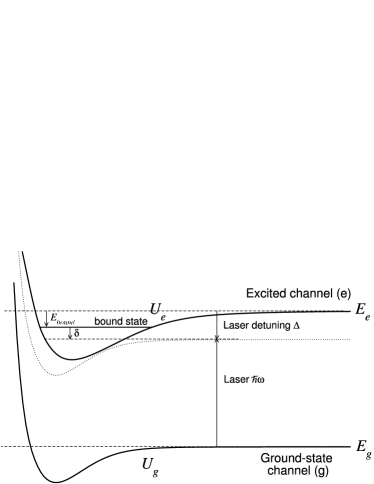
Figure 1: Scheme of the photoassociation process

Let us now turn to the standard two-channel model describing the photoassociation reaction in a thermal gas of atoms, schematized in Fig. 1, with a ground potential $U_{\text{g}}(r)$, an excited potential $U_{\text{e}}(r)+E_{e}$ and a time-dependent radiative coupling due to a laser red-detuned by $\hbar\Delta$ relative to an atomic resonance line. We assume that $U_{\text{e}}(\infty)\rightarrow E_{e}$, $U_{\text{g}}(\infty)\rightarrow 0$, $E_{e}$ being the dissociation limit of the excited potential, while the origin of energy is the dissociation limit of the ground potential. The relative motion of two atoms is described by a two-component wave function $\Phi$, with $F_{\text{ground}}(\mathbf{r},t)$ describing two atoms colliding in the potential $U_{\text{g}}$ (open channel), and $F_{\text{exc}}(\mathbf{r},t)$ describing the ro-vibrational motion in the excited potential $U_{\text{e}}$ (closed channel). For a continuous laser with constant frequency $\omega$ such that $\hbar\omega=\hbar\omega_{0}-\Delta$, in a classical model, the electric field oscillates as $\cos(\omega t)$ and is coupled with the transition dipole moment $\mathbf{D}(r)$ between the two electronic states. At low temperature, only $s$-wave scattering should be considered, and we shall neglect rotation effects and transfer of angular momentum between the light field and the pair of atoms, so that instead of ($F_{\text{ground}}(\mathbf{r},t)$, $F_{\text{exc}}(\mathbf{r},t)$) only radial functions $\phi_{\text{g}}(r,t)$, $\phi_{\text{exc}}(r,t)$ need to be introduced. Using the rotating wave approximation Allen and Eberly (1987), it is possible to eliminate the rapid oscillations in the coupling term by defining new wave functions

$$\phi_{\text{e}}(r,t)=\exp(i\omega t)\phi_{\text{exc}}(r,t)$$ (35)

so that the the time-dependent Schrödinger equation becomes Luc-Koenig et al. (2004a)

$$i\hbar\frac{\partial}{\partial t}\left(\!\begin{array}[]{c}\phi_{g}(r,t)\\ \phi_{e}(r,t)\end{array}\!\right)$$ (38)

$$=\left(\!\begin{array}[]{lc}\hat{\mathbf{T}}+U_{g}(r)&W(r,t)\\ W(r,t)&\hat{\mathbf{T}}+U_{e}(r)+E_{e}-\hbar\omega\end{array}\!\right)\left(\!\begin{array}[]{c}\phi_{g}(r,t)\\ \phi_{e}(r,t)\end{array}\!\right)$$ (43)

where we have introduced the kinetic energy operator $\hat{\mathbf{T}}$ and a coupling term:

$$W(r,t)\approx W(t)=-\frac{1}{2}\sqrt{\frac{2I(t)}{c\epsilon_{0}}}D.$$ (44)

$I(t)$ is the intensity of the laser, the constants $c$ and $\epsilon_{0}$ are respectively the ligth velocity and the vacuum permittivity, and $D$ is one component of the dipole moment operator, depending upon the polarisation of the laser, and assumed to be $r$-indedependent. Since $E_{e}-\hbar\omega$=$\Delta$, the 2-channel Hamiltonian in (38) reads

$$\mathbf{H}^{(2)}(r,t)=\left(\begin{array}[]{lc}\hat{\mathbf{T}}+U_{g}(r)&W(t)\\ W(t)&\hat{\mathbf{T}}+U_{e}(r)+\Delta\end{array}\right)$$ (45)

The relevant quantities for the photoassociation reaction are illustrated in Fig. 1.

III.2 Coupled equations for a condensate

Considering now photoassociation in a condensate, we treat the many-body problem with a two-component pair wave function $\Phi$: the usual component $\Phi_{\text{g}}$ in the ground (open) channel, and a new component $\Phi_{\text{e}}$ in the excited (closed) channel. The component in the open channel is connected at large distances to a product of condensate wave functions $\Psi$, whereas the component in the closed channel corresponds to a bound vibrational level and vanishes at large distances,

$$\Phi(\mathbf{x,y},\!t)=\left(\!\!\!\begin{array}[]{c}\Phi_{\text{g}}(\mathbf{x,y},\!t)\\ \Phi_{\text{e}}(\mathbf{x,y},\!t)\end{array}\!\!\!\right)\xrightarrow[|\mathbf{x-y}|\rightarrow\infty]{\;}\left(\!\!\!\begin{array}[]{c}\Psi(\mathbf{x},\!t)\Psi(\mathbf{y},\!t)\\ 0\end{array}\!\!\!\right)$$

For simplicity, we will consider a homogeneous system. In this case, the condensate wave function $\Psi(\mathbf{x},t)$ is uniform, and the functions $\Phi(\mathbf{x,y},t)$ and $R^{\prime}(\mathbf{x,y},t)$ depend only on the relative coordinate $\mathbf{x-y}$ = $\mathbf{r}$. Assuming an isotropic situation with s-wave scattering only we shall simply write $\Psi(t)$, $\Phi_{g}(r,t)$, $\Phi_{e}(r,t)$ and $R^{\prime}(r,t)$ for the condensate wave function, the two components of the pair wave function, and the density matrix for the non-condensate atoms in the ground state.

III.2.1 Coupled equations in the first-order cumulant approximation

The first-order cumulant equations (16-17) are generalized as follows Gasenzer (2004):

$$i\hbar\frac{\partial\Psi(t)}{\partial t} = M(t)\Psi(t)$$ (46)

$$i\hbar\frac{\partial}{\partial t}\left(\!\!\begin{array}[]{c}\Phi_{\text{g}}(r,t)\\ \Phi_{\text{e}}(r,t)\end{array}\!\!\right) = \bigg{(}\mathbf{H}^{(2)}(r,t)\bigg{)}\!\cdot\!\left(\!\!\begin{array}[]{c}\Phi_{\text{g}}(r,t)\\ \Phi_{\text{e}}(r,t)\end{array}\!\!\right)$$ (54)

$$+\;2M(t)\left(\!\!\begin{array}[]{c}\Psi^{2}(t)\\ 0\end{array}\!\!\right)$$

with the mean field:

$$M(t)=\frac{1}{\Psi(t)}\int\!\!d^{3}\textbf{r}\Psi^{*}(t)\Big{(}U_{\text{g}}(r)\Phi_{\text{g}}(r,t)+W(r,t)\Phi_{\text{e}}(r,t)\Big{)}$$ (55)

now depending upon the radiative coupling besides the ground state potential, and upon both components of the pair wave function. From $M(t)$ one can deduce a mean-field scattering length through

$$a_{M}(t)=M(t)\frac{m}{4\pi\hbar^{2}|\Psi(t)|^{2}}.$$ (56)

The conservation equation reads

$$\rho=\rho_{\text{g}}(t)+\rho_{\text{g}}^{\prime}(t)+\rho_{\text{e}}(t)$$ (57)

where $\rho$ is the total density, $\rho_{\text{g}}(t)=|\Psi(t)|^{2}$ is the density of condensate atoms in the initial channel, $\rho_{\text{g}}^{\prime}(t)=R^{\prime}(0,t)$ is the density of non-condensate atoms in the initial channel, and $\rho_{e}=4\pi\int\!\!|\Phi_{\text{e}}(r,t)|^{2}r^{2}dr$ is the density of atoms in the excited (molecular) channel. Furthermore, we still have in the ground channel the “approximate Bogoliubov relation" (24), which now reads:

$$R^{\prime}(r,t)=\int\!\!d^{3}\mathbf{z}\;\Phi_{\text{g}}^{\prime*}(\mathbf{z},t)\Phi_{\text{g}}^{\prime}(\mathbf{r-z},t).$$ (58)

and links the density matrix for the non-condensate atoms to the correlated part of the component of the pair wave function in the ground channel.

III.2.2 Coupled equations in the reduced pair wave approximation

The generalized form of Eqs. (28-29) is

$$i\hbar\frac{\partial\Psi(t)}{\partial t} \!\!=\!\! M(t)\Psi(t)$$ (59)

$$i\hbar\frac{\partial}{\partial t}\left(\!\!\begin{array}[]{c}\Phi_{\text{g}}(r,t)\\ \Phi_{\text{e}}(r,t)\end{array}\!\!\right) \!\!=\!\! \left(\!\mathbf{H}^{(2)}(r,t)+\!\left(\!\!\begin{array}[]{lc}2M(t)&0\\ 0&0\end{array}\!\!\right)\!\right)\!\cdot\!\left(\!\!\begin{array}[]{c}\Phi_{\text{g}}(r,t)\\ \Phi_{\text{e}}(r,t)\end{array}\!\!\!\right)\qquad$$ (66)

with the mean field $M(t)$ still defined by Eq. (55). The conservation equation (57) still holds, but the Bogoliubov relation (58) is no longer valid.

III.3 Introduction of the spontaneous emission

When a pair of atoms in a confining trap is photoassociated, populating a bound vibrational level of the potential $U_{e}(r)$, the excited molecule has a finite lifetime and decays back to the ground electronic state by spontaneous emission of a photon. Most often, the final state is a continuum level of the ground potential $U_{g}(r)$, where the pair of atoms has enough energy to escape the trap. In some cases, the radiative transition populates a bound level of $U_{g}(r)$, leading to the formation of stable molecules Fioretti et al. (1998); Masnou-Seeuws and Pillet (2001).

In the previous equations, decay by spontaneous emission is not considered. Assuming that it is mainly a loss phenomenon, it can be accounted for by adding an imaginary term to the excited potential $U_{e}(r)$,

$$U_{e}(r)\rightarrow U_{e}(r)-i\frac{\hbar\gamma}{2},$$ (67)

where $2\pi/\gamma$ is the radiative lifetime of the bound levels in the excited potential (we have assumed the dipole moment to be $r$-independent). The component of the pair wave function in the closed channel therefore contains an exponentially decreasing factor: as a result, the total density (57) is no longer conserved during the time evolution.

IV Mean-field equations and Rogue dissociation

As a general rule, the coupled mean-field (Gross-Pitaevskiĭ) equations of Ref. Timmermans et al. (1999) are retrieved from both approximations when the pair dynamics can be eliminated adiabatically with respect to the one-body dynamics Naidon and Masnou-Seeuws (2003). However the adiabaticity condition given in Paper I Naidon and Masnou-Seeuws (2003) (merely comparing the coupling constants in the equations) has to be refined. We give here a more relevant condition, related to the rogue dissociation analysis of Ref. Javanainen and Mackie (2002).

Let us first assume that only one excited molecular level is resonant. In this case, we call $\delta$ the detuning of the laser from this molecular level (see Fig. 1). One can write $\Phi_{e}(r,t)\approx\sqrt{2}\Psi_{m}(t)\varphi_{m}(r)$, where $\varphi_{m}(r)$ is the volume-normalized wave function for the relative motion in this resonant molecular level and $\Psi_{m}(t)$ is the (here uniform) centre-of-mass wave function corresponding to a molecular condensate. With this normalization, $|\Psi_{m}|^{2}$ is the density of molecules.

Then, the crucial point is to write the correlation in the pair wave function as a sum of an adiabatic correlation and a dynamic correlation

$$\Phi_{g}(r,t) = \Psi^{2}(t)+\Phi_{g}^{ad}(r,t)+\Phi_{g}^{dyn}(r,t)$$

$$= \Psi^{2}(t)\left(1+\varphi_{g}^{ad}(r,t)+\varphi_{g}^{dyn}(r,t)\right).$$

The adiabatic part is found by setting $\Phi_{g}^{dyn}$ and $\frac{\partial}{\partial t}\Phi_{g}^{ad}$ to zero in Eq. (54) or $\varphi_{g}^{dyn}$ and $\frac{\partial}{\partial t}\varphi_{g}^{ad}$ to zero in Eq. (66). We can then expand the correlation in terms of the scattering states $|\varphi_{\textbf{k}}\rangle$ of the ground potential $U_{g}$ :

$$\Phi_{g}(r,t) = \Psi^{2}(t)+\int\!\!\!\!\!\begin{array}[]{c}\frac{d^{3}\textbf{k}}{(2\pi)^{3}}\end{array}\left(C_{\textbf{k}}^{ad}(t)+C_{\textbf{k}}^{dyn}(t)\right)\varphi_{\textbf{k}}(r)$$

with the normalization $\langle\varphi_{\textbf{k}}|\varphi_{\textbf{q}}\rangle=(2\pi)^{3}\delta^{3}(\textbf{k-q})$ . We find:

$$C_{\textbf{k}}^{ad}(t)=-\frac{m}{\hbar^{2}k^{2}}\left(g_{\textbf{k}}\Psi^{2}+w_{\textbf{k}}\Psi_{m}\right).$$ (69)

Eliminating this adiabatic part in Eqs. (46-54) or (59-54) leads to the terms of the mean-field equations Naidon and Masnou-Seeuws (2003). The equations for $\Psi$ and $\Psi_{m}$ then read:

$$i\hbar\dot{\Psi} \!=\! \Psi^{*}\left[\left(g_{0}\Psi^{2}+\int\!\!\!\!\!\begin{array}[]{c}\frac{d^{3}\textbf{k}}{(2\pi)^{3}}\end{array}g_{\textbf{k}}C_{\textbf{k}}^{dyn}\right)+w\Psi_{m}\right]$$ (71)

$$i\hbar\dot{\Psi}_{m} \!=\! \hbar(\delta^{\prime}\!-\!i\frac{\gamma}{2})\Psi_{m}+\!\frac{1}{2}\!\!\left(\!w_{0}\Psi^{2}\!+\!\!\int\!\!\!\!\!\begin{array}[]{c}\frac{d^{3}\textbf{k}}{(2\pi)^{3}}\end{array}w_{\textbf{k}}C_{\textbf{k}}^{dyn}\!\right)\quad$$ (73)

where

• $g_{\textbf{k}}=\int d^{3}rU(r)\varphi_{\textbf{k}}(r)$ is the atom-atom scattering coupling constant (in particular $g_{0}=\frac{4\pi\hbar^{2}a}{m}$)

• $w_{\textbf{k}}=\sqrt{2}\langle\varphi_{\textbf{k}}|W|\varphi_{m}\rangle$ is the atom-molecule coupling constant

• $\delta^{\prime}=\delta+E_{self}$ is the detuning shifted by the self-energy of the molecules

The equation for the dynamic correlation in the first-order cumulant approximation is:

$$i\hbar\dot{C}_{\textbf{k}}^{dyn}=\frac{\hbar^{2}\textbf{k}^{2}}{m}C_{\textbf{k}}^{dyn}-i\hbar\dot{C}_{\textbf{k}}^{ad}$$ (74)

and in the reduced pair wave approximation:

$$i\hbar\dot{c}_{\textbf{k}}^{dyn}=\frac{\hbar^{2}\textbf{k}^{2}}{m}c_{\textbf{k}}^{dyn}-i\hbar\dot{c}_{\textbf{k}}^{ad}$$ (75)

with $c_{\textbf{k}}=C_{\textbf{k}}/\Psi^{2}$. As long as the momentum distribution of $C_{\textbf{k}}^{dyn}$ lies in the Wigner’s threshold regime, we can make the simplification: $g_{\textbf{k}}\approx g_{0}$ and $w_{\textbf{k}}\approx w_{0}$. Note that this approximation does not lead to any ultraviolet divergence, because we have eliminated the adiabatic correlation beforehand. Such an approximation, reminiscent of the use of a contact potential, would have given rise to ultraviolet divergences if we had made it in the original equations (46-54) or (59-54).

It is now clear from Eqs. (71-73), that when the dynamic correlation $C_{\textbf{k}}^{dyn}$ is negligible, one gets the Gross-Pitaevskiĭ equations of Ref. Timmermans et al. (1999):

$$i\hbar\dot{\Psi} = g_{0}|\Psi|^{2}\Psi+w_{0}\Psi^{*}\Psi_{m}$$ (76)

$$i\hbar\dot{\Psi}_{m} = \hbar(\delta^{\prime}-i\frac{\gamma}{2})\Psi_{m}+\frac{1}{2}w_{0}\Psi^{2}$$ (77)

The mean-field approximation will break down when the dynamic correlation is not negligible any more. This means that molecules break into pairs of atoms which will contribute to the non-condensate fraction instead of the condensate fraction. From Eqs. (71-73) we see that such rogue dissociation Javanainen and Mackie (2002) can be neglected as long as:

$$\left|\int\!\!\!\!\!\begin{array}[]{c}\frac{d^{3}\textbf{k}}{(2\pi)^{3}}\end{array}C_{\textbf{k}}^{dyn}\right|\ll\left|\Psi^{2}\right|$$ (78)

To give a more explicit condition, we first have to make a distinction between two different regimes of Eqs. (76-77).

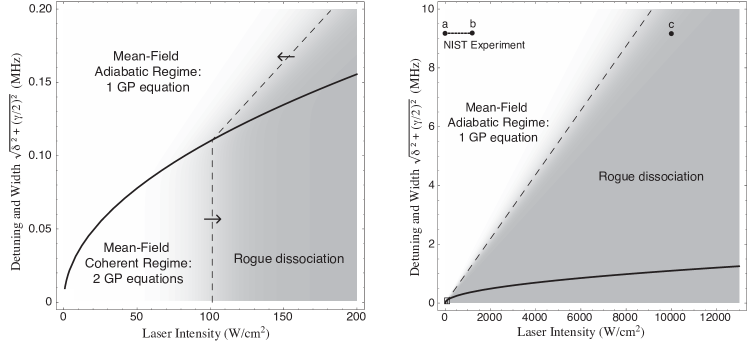
Figure 2: Different regimes of photoassociation in a condensate, as a function of laser intensity and the combined effect of detuning and spontaneous emission. These graphs correspond to the sodium resonance described in VI.1, for a density of $4\times 10^{14}$at/cm³, but spontaneous emission is taken as a free parameter. Left panel: the solid line is the limit between the adiabatic regime and the coherent regime of the mean-field equations (76-77). The mean-field approximation is valid in the white areas, and rogue dissociation occurs in the shaded areas. The vertical dashed lines corresponds to the left hand side of (85) being equal to $\pi^{2}$ and the oblique dashed line corresponds to the left hand side of (86) being equal to $\pi^{2}$. The arrows indicate how these lines move when the density is increased. Right panel: larger view showing the experimental investigation of Ref. McKenzie et al. (2002) (from dot a to dot b) where the spontaneous emission parameter $\gamma/2$ is equal to $2\pi\times$9.18 MHz; dot c corresponds to the condition of our numerical investigation described in VI.3.

IV.1 The adiabatic regime

We consider the limit when $|i\hbar\dot{\Psi}_{m}|\ll|\frac{1}{2}w_{0}\Psi^{2}|$. In this case, $\Psi_{m}$ can be eliminated adiabatically, so that:

$$\Psi_{m}\approx-\frac{w_{0}}{2\hbar(\delta^{\prime}-i\frac{\gamma}{2})}\Psi^{2}$$ (79)

and:

$$i\hbar\dot{\Psi}\approx\big{(}g-\frac{w_{0}^{2}}{2\hbar(\delta^{\prime}-i\frac{\gamma}{2})}\big{)}|\Psi|^{2}\Psi\equiv\frac{4\pi\hbar^{2}a_{M}}{m}|\Psi|^{2}\Psi$$ (80)

In this regime, the coupled equations reduce to a single Gross-Pitaevskiĭ equation Timmermans et al. (1999); Mackie et al. (2002) where the mean-field scattering length $a_{M}$ corresponds to the modified scattering length:

$$A=a+a_{\text{opt}}+ib_{\text{opt}}$$

given by the two-body theory of the resonance Fedichev et al. (1996); Bohn and Julienne (1997). Therefore, most physical properties can be described by the usual two-body theory. For instance, Eq. (80) implies that the atomic density $\rho_{g}=|\Psi|^{2}$ follows a simple rate equation:

$$\dot{\rho}_{g}=-\frac{8\pi\hbar b_{\text{opt}}}{m}\rho_{g}^{2}$$ (81)

and using (69) and (79), one can calculate the pair wave function and find the usual asymptotic behaviour:

$$\Phi_{g}(r,t)\xrightarrow[r\to\infty]{}\Psi^{2}(t)\left(1-\frac{a_{M}}{r}\right)$$ (82)

As a matter of fact, the molecular field $\Psi_{m}$ scales as $\rho$ in this regime: it is merely a two-body field playing the role of an intermediate state during the collision process. Using (79) and (80), we find that the condition $|i\hbar\dot{\Psi}_{m}|\ll|\frac{1}{2}w_{0}\Psi^{2}|$ is satisfied whenever:

$$\hbar|\delta^{\prime}+i\frac{\gamma}{2}|\gg w_{0}\sqrt{\rho},\;2g\rho$$ (83)

This corresponds to the off-resonant regime of Ref. Timmermans et al. (1999): the detuning and the spontaneous emission are large with respect to the coherent couplings.

IV.2 The coherent regime

On the other hand, we may consider the limit $|\hbar(\delta^{\prime}-i\frac{\gamma}{2})\Psi_{m}|\ll|\frac{1}{2}w_{0}\Psi^{2}|$ and $|g_{0}|\Psi|^{2}\Psi|\ll|w_{0}\Psi^{*}\Psi_{m}|$. In this case, the solutions of Eqs. (76-77) for an initially all atomic system are:

$$\Psi \approx \sqrt{\rho}/\cosh(w_{0}\sqrt{\rho}t)$$

$$\Psi_{m} \approx -i\sqrt{\rho}\tanh(w_{0}\sqrt{\rho}t)$$

There is a coherent conversion between atoms and molecules. In this regime, $\Psi_{m}$ scales as $\sqrt{\rho}$ and plays the role of a one-body field, i.e. a molecular condensate in its own right. As a result, the system cannot be described by a two-body theory any more. For instance, the pair wave function is still of the form (82), but the mean-field scattering length $a_{M}$ is now a time-dependent quantity $a-iL\sinh(2w_{0}\sqrt{\rho}t)$ where:

$$L=\frac{m}{4\pi\hbar}\frac{w_{0}}{2\sqrt{\rho}}$$

is a many-body length which depends on the density. This means that the density of atoms does not follow a rate equation.

We find that this coherent regime occurs when:

$$w_{0}\sqrt{\rho}\gg\hbar|\delta^{\prime}+i\frac{\gamma}{2}|,\;2g\rho$$ (84)

In practice, while it is possible to set the detuning to zero by varying the laser frequency, the spontaneous decay $\gamma$ is fixed by the molecular level of the system. Spontaneous emission in alkali systems, and loss processes in general, make it very difficult to reach the coherence condition (84) with realistic densities and laser intensites. For this reason, photoassociation experiments in condensates so far McKenzie et al. (2002); Theis et al. (2004); Winkler et al. (2005) have been confined to the adiabatic regime (83), and can be described simply by two-body theories.

However, we made some estimates which indicate that photoassociation for weakly-allowed transitions, such as those found in alkaline-earth dimers, would lead to the coherent regime. The reason is that spontaneous emission scales as the square of the dipole moment whereas the coherent coupling $w_{0}\sqrt{\rho}$ only scales as the dipole moment.

IV.3 Rogue dissociation

In the coherent regime, which is the regime originally investigated in Ref. Javanainen and Mackie (2002), the relevant energy scale set by the dynamics is $\hbar\Omega=w_{0}\sqrt{\rho}$ defining the coherent Rabi frequency $\Omega/2\pi$. As a result, Eq. (74) or (75) can be made dimensionless using the characteristic time $\tau=\Omega^{-1}$ and length $\xi=\sqrt{\hbar/m\Omega}=(4\pi L\rho)^{-1/2}$. Since $|\Psi|^{2}\sim\rho$ and $|C_{\textbf{k}}^{dyn}|\sim 1$, the rogue dissociation condition (78) can be written:

$$\left(\rho\xi^{3}\right)^{-1}=\left(\frac{\hbar\Omega}{\frac{\hbar^{2}\rho^{2/3}}{m}}\right)^{3/2}=\left((4\pi L)^{3}\rho\right)^{1/2}\ll 2\pi^{2}$$ (85)

This condition was presented in J. Javanainen and M. Mackie’s work Javanainen and Mackie (2002).

Similarly, in the adiabatic regime, the relevant energy scale is $\hbar\Gamma=w_{0}^{2}\rho/\sqrt{\delta^{\prime 2}+(\gamma/2)^{2}}$ corresponding to the mean field energy $\hbar\Gamma=\frac{4\pi\hbar^{2}|A|}{m}\rho$. Eq. (74) or (75) can be made dimensionless using the characteristic time $\tau_{0}=\Gamma^{-1}$ and length $\xi_{0}=\sqrt{\hbar/m\Gamma}=(4\pi|A|\rho)^{-1/2}$ (note that this is the usual healing length), and the rogue dissociation condition is now:

$$\left(\rho\xi_{0}^{3}\right)^{-1}=\left(\frac{\hbar\Gamma}{\frac{\hbar^{2}\rho^{2/3}}{m}}\right)^{3/2}=\left((4\pi|A|)^{3}\rho\right)^{1/2}\ll 2\pi^{2}$$ (86)

Both conditions (85) and (86) can be written as $\sqrt{\rho a_{M}^{3}}\ll 1$ which is a straightforward generalization of the usual condition $\sqrt{\rho a^{3}}\ll 1$ for the validity of the Gross-Pitaevskiĭ equation. This can be interpreted as follows: rogue dissociation occurs when the average spacing $\rho^{-1/3}$ between the atoms becomes of the order of the typical length associated to the adiabatic correlation, either $A$ in the adiabatic regime, or $L$ in the coherent regime. However, there is a fondamental difference. $A$ is the modified scattering length, a two-body quantity independent of the density; in the adiabatic regime, one can thus reach the rogue dissociation regime by increasing the density, so that the average spacing between the atoms becomes of the order of $A$. The mean-field equations are therefore valid at low density in the adiabatic regime. On the other hand, in the coherent regime, the many-body length $L$ decreases with density, and more rapidly than the average spacing between the atoms. As a result, one should decrease the density to observe rogue dissociation. The mean-field equations are therefore valid at high density in the coherent regime. An overview of the different regimes and conditions is given in Fig. 2.

V Numerical methods and calculations

We now turn to the numerical resolution of the time-dependent equations (46-54) and (59-66). The main difficulty is that they describe simultaneously the microscopic dynamics, with short characteristic times, and the macroscopic dynamics, with longer ones. At each time step, the mean field $M(t)$ and the mean-field scattering length $a_{M}(t)$ must be determined through Eqs. (55,56), from the two components of the pair wave function $\Phi_{\text{g}}(r,t)$ and $\Phi_{\text{e}}(r,t)$ and from the condensate wave function $\Psi(t)$. Then the mean field influences the evolution of the three wave functions in the coupled equations (46,54) or (59,66). Note that in previous calculations based on the cumulant equations Gasenzer (2004), the use of a non-local, separable potential made it possible to first perform an independent integration of the two-body equation (66), then inject the results into the condensate equation to solve a non-Markovian non-linear Schrödinger equation. This simplifying procedure is not implemented in the present paper where we use the same realistic potentials in both approaches.

The pair wave functions are represented on a grid, using a mapping procedure where the grid steps are adjusted to the local de Broglie wavelengths Kokoouline et al. (1999) in the two potentials, choosing the smallest of the two values at a given $r$. The short range oscillations are thus described with a dense grid and the long range behaviour with a diffuse one. Typical value of the grid length $L$ is 200,000 $a_{0}$. The whole set of equations, either (46-54) or (59-66)) are then solved, using the standard Crank-Nicholson method Press et al. (1996) for the propagation in time. The solutions at $t=0$ are chosen as stationary solutions for the open (ground) channel, when no laser coupling is present.

V.1 Initial state in the first-order cumulant approximation

Stationary solutions (in the rotating frame defined by Eq. (35)) of Eqs. (46-54) are given by

$$\bar{\Psi} = \sqrt{\bar{\rho}_{\text{g}}}$$ (87)

$$\left(\!\!\begin{array}[]{c}\bar{\Phi}_{\text{g}}(r,t)\\ \bar{\Phi}_{\text{e}}(r,t)\end{array}\!\!\right) = -\bigg{(}\!\mathbf{H}^{(2)}(r,t)\!-2\mu\bigg{)}^{-1}\!\cdot\!2\mu\left(\!\!\begin{array}[]{c}\bar{\rho}_{\text{g}}\\ 0\end{array}\!\!\right)$$ (92)

where $\bar{\rho}_{\text{g}}$ is the initial condensate density, and $\mu=\bar{M}$ is the chemical potential (equal to the initial mean field in the present case). When the laser is initially off, the coupling term $W$ in $\mathbf{H}^{(2)}$ is zero. To compute (87-92), we start from a given value for the condensate density $\bar{\rho}_{\text{g}}$ and a guess value for $\mu$. We determine the pair wave function from (92) by performing a matrix inversion. This gives a new value of the mean field through Eq. (55), and the procedure is iterated until convergence is reached for $\mu$. As explained in Section II, for certain values of the density $\bar{\rho}_{\text{g}}$, the matrix is singular and the solution shows an unphysical resonance of the mean-field scattering length. Between the resonances the mean-field scattering length is essentially equal to the expected scattering length of the two-atom system. This difficulty is illustrated in Fig. 3. We therefore choose an initial density that is both close to the experimental value and such that the mean-field scattering length does lie in-between the resonances.

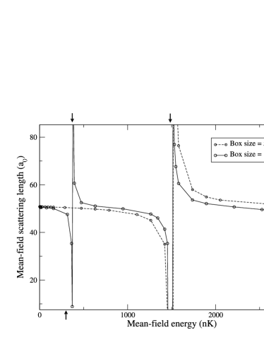
Figure 3: Mean-field scattering length as defined from Eqs. (55-56), calculated from the stationary solution of the first-order cumulant equations (16, 17), as a function of the mean-field energy. The numerical calculations shown here correspond to the case of a sodium condensate without any photoassociation laser, and are performed within a square box of width $d$= 10,000 a₀ (solid lines) or $d$=5,000 a₀ (dashed line). The position of the first two levels of the wider box are indicated by arrows on the upper horizontal axis, the second one coinciding with the first level of the $d$=5,000 box. As explained in the text, the mean-field scattering length has an unphysical divergence each time the mean-field energy coincides with an energy level of the box. The latter depend on the arbitrary size the box; in our calculations, this size can typically go up to 200,000 atomic units, which increases the number of resonances. The typical mean-field energy in the experiment of Ref. McKenzie et al. (2002) is about 6 kHz $\approx$ 300 nK, and indicated by an arrow on the lower horizontal axis.

V.2 Initial state in the reduced pair wave approximation

Stationary solutions of Eqs. (59-66) are obtained by solving

$$\bar{\Psi} = \sqrt{\bar{\rho}_{g}}$$ (93)

$$0 = \left(\!\mathbf{H}^{(2)}(r,t)\!-\!\left(\!\!\begin{array}[]{cc}0&0\\ 0&2\mu\end{array}\!\!\right)\right)\!\cdot\!\left(\!\!\begin{array}[]{c}\bar{\Phi}_{\text{g}}(r,t)\\ \bar{\Phi}_{\text{e}}(r,t)\end{array}\!\!\right)$$ (98)

The two-component function $(\bar{\Phi}_{\text{g}},\bar{\Phi}_{\text{e}})$ is therefore the zero energy stationary solution of the two-channel problem, the potential $U_{e}$ being shifted down by twice the chemical potential. This means that the energy of the optically induced Feshbach resonance is shifted by the mean-field energy of the condensate atoms, even though the collision energy is nearly zero. To determine eigenfunctions of Eq. (98) we propagate Eq. (66) in imaginary time with the Crank-Nicholson scheme Press et al. (1996). The finite value of the time step value acts as an energy filter, which selects the zero energy scattering state in a few steps.

V.3 Accuracy check: computation of the scattering length

Checks on the macroscopic dynamics can be performed by comparing with the mean-field equations (76-77) when rogue dissociation is negligible (see below). As for the microscopic dynamics, we have to ensure that the mean-field scattering length (56), deduced from the integral expression (55), is computed accurately enough at each time step. To that purpose, we have solved the stationary version of the two-body equations (38) and extracted the phase shift of the continuum wave function in the open channel from its asymptotic behaviour. The scattering length can be deduced by extrapolation to zero collision energy. In Fig. 4, we compare the scattering length computed by this method, and the mean-field scattering length given by Eq. (55). One can see from the excellent agreement that the latter is indeed accurately computed in the stationary case.

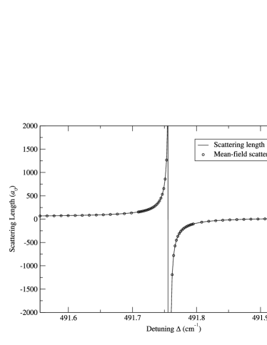
Figure 4: Optically induced Feshbach resonance: variation of the sodium scattering length as a function of the detuning of the photoassociation laser in the vicinity of the $v$=135, $J$=1 resonance McKenzie et al. (2002), for a laser intensity of 15 kW/cm², and a variable detuning $\Delta$ relative to the D₁ atomic resonance line. Spontaneous emission is not included in these calculations. Solid line: scattering length determined by phase shift from two-atom calculations. Dots: mean-field scattering length as defined by Eqs. (55-56), calculated from the stationary states in the reduced pair wave approximation, see Eq. (93-98).

VI Application: photoassociation in a sodium condensate

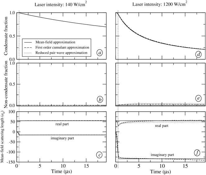
Figure 5: On-resonance photoassociation dynamics for the $v$=135 level of Na₂ A${}^{1}\Sigma_{u}^{+}$ using a cw laser of intensity (for $t>0.5\mu$s) $I$= 140 W/cm² (left column) and $I$=1200 W/cm² (right column). This corresponds to the adiabatic regime where all approximations reduce to the mean-field aproximation and are consistent with usual two-body theory. Top panels (a) and (d): the decay of the condensate fraction $\alpha_{\text{g}}(t)$ is caused by spontaneous emission and dissociation of the photoassociated molecules into pairs of atoms which escape the trap. This decay is more rapid in panel (d), due to the larger intensity (1200 W/cm²) of the photoassociation laser. Middle panels (b) and (e): time variation of the fraction of non-condensate ground state atoms $\alpha_{\text{g}}^{\prime}(t)$, which remains negligible. Bottom panels (c) and (f): time variation of the real $\Re[a(t)]$ and imaginary $\Im[a(t)]$ part of the mean-field scattering length.

VI.1 Experimental conditions of the NIST experiment

The chosen example starts from the photoassociation experiment in NIST McKenzie et al. (2002), where a condensate of sodium atoms is illuminated by a cw laser of intensity $I$ varying from 0.14 to 1.20 kW/ cm². The peak density is about $4\times 10^{14}$at/cm³. The frequency ( 16 913.37 cm^-1) is chosen at resonance with the $J$=1, $v$=135 vibrational level in the 0${}_{u}^{+}$ ($3S+3P_{1/2}$) potential curve of Na₂. The detuning of the photoassociation laser relative to the D₁ resonance line is rather large (43 cm^-1), and corresponds to the binding energy of the $v$=135 level. The molecules formed in the excited electronic state have a natural width $\gamma=2\pi\times 18.38$ MHz due to spontaneous emission.

Previous estimations McKenzie et al. (2002) based on criterion (85) Javanainen and Mackie (2002) predicted that these experimental conditions should lead to rogue dissociation, as $\left(2\pi^{2}\rho\xi^{3}\right)^{-1}\approx 3.2$ for $I=1.2$ kW/cm². However, this criterion is relevant only in the coherent regime. According to the analysis of section IV, the experiment is actually in the adiabatic regime (see Fig. 2), as $2\Omega/\gamma\sim 0.04$. Therefore, the relevant criterion is (86). As $\left(2\pi^{2}\rho\xi_{0}^{3}\right)^{-1}\approx 0.03$ for $I=1.2$ kW/cm², one concludes that no rogue dissociation should occur and the mean-field approximation should be valid, which is consistent with the experimental observation. However, if the intensity can be increased up to $10$ kW/cm², then $\left(2\pi^{2}\rho\xi_{0}^{3}\right)^{-1}\approx 0.6$ and rogue dissociation should occur (see Fig. 2). We therefore present numerical calculations simulating the experiment in this high-intensity regime to see the effects of rogue dissociation. Calculations in similar conditions were done by T. Gasenzer Gasenzer (2004) using the first-order cumulant equations with separable potentials.

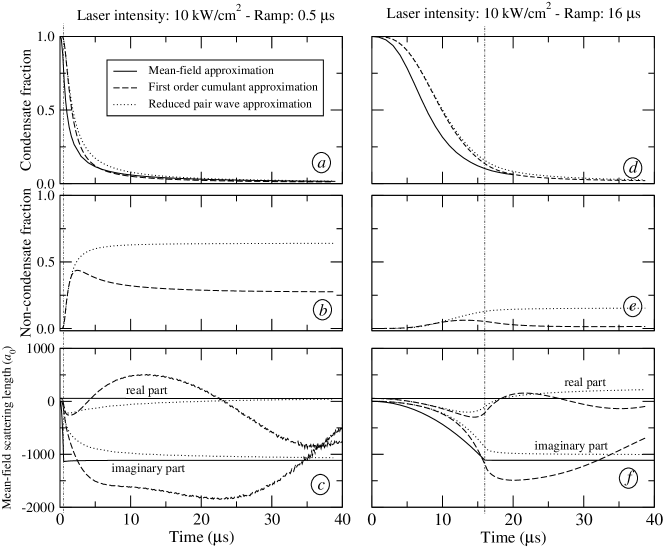
Figure 6: Same as Fig. 5 for an intensity of 10 kW/cm². Left column corresponds to a rise time of the laser of 0.5 $\mu s$, whereas right column corresponds to a rise time of 16 $\mu s$ (the end of the ramp is indicated by a dotted-dashed vertical line).

VI.2 Parameters of the calculations

For these calculations, the potentials curves for the ground state of Na₂ X${}^{1}\Sigma_{g}^{+}$ and $0_{u}^{+}$(3s+3p${}_{1/2})$ have been taken from Ref. Pellegrini (2003). The ground state potential is chosen so that the scattering length is 54.9 a₀, as in T. Gasenzer’s work Gasenzer (2004). Hyperfine structure is not included, and the last bound level has a binding energy of 317.78 MHz ( $\sim 10^{-2}$ cm^-1). In the excited curve, the level $v$=135 is bound by 49.23 cm^-1, the two neighbouring levels being $v$=134 at -52.95 cm^-1 and $v$=136 at -45.757 cm^-1. The spontaneous emission term (67) for this excited state is set to $\gamma=2\pi\times 18.36$ MHz to match the experiment McKenzie et al. (2002).

The dipole moment matrix element is taken as $D$=2, assuming linear polarisation of the laser, neglecting $r$-dependence, and deducing the atomic lifetime from the long range coefficient $C_{3}$= 6.128 of Marinescu and Dalgarno Marinescu and Dalgarno (1995). The coupling term $W$ in the equations (38) is therefore linked to the intensity I by $W=\sqrt{2I/(c\epsilon_{0})}$.

We model the cw laser as follows: the intensity starts from zero and is turned on linearly ($I_{b}(t)=I\times t/T;\,\,t\leq T$) to become constant and equal to $I$ after $t=T=0.5\mu$s. This value of $T$, previously used in the calculations by T. Gasenzer Gasenzer (2004), corresponds to the typical rise and fall-off times of the laser in the experiment of Ref. McKenzie et al. (2002). Starting from a pure sodium condensate, with a density $\rho(t=0)$=$\rho_{\text{g}}(t=0)$, and therefore assuming $\rho^{\prime}(t=0)$=$\rho_{\text{e}}(t=0)=0$, we have solved the coupled equations (46,54) and (59, 66) as well as the mean-field equations (76-77). From these calculations, we obtain the time-variation of the relative number of condensate atoms

$$\alpha_{\text{g}}(t)=\rho_{\text{g}}(t)/\rho(0);\,\,\alpha_{\text{g}}(0)=1,$$ (99)

of non-condensate atoms in the open channel,

$$\alpha_{\text{g}}^{\prime}(t)=\rho_{\text{g}}^{\prime}(t)/\rho(0);\alpha_{\text{g}}^{\prime}(0)=0$$ (100)

and the relative number of atoms in the closed channel

$$\alpha_{\text{e}}(t)=\rho_{\text{e}}(t)/\rho(0)=2\beta_{\text{e}}(t);\,\,\beta_{\text{e}}(0)=0,$$ (101)

which is twice the relative number of photoassociated molecules $\beta_{\text{e}}(t)$. The remaining fraction $1-\alpha_{\text{g}}-\alpha_{\text{g}}^{\prime}-\alpha_{\text{e}}$ corresponds to photoassociated molecules that have been deexcited by spontaneous emission, yielding either cold molecules in the ground state or pairs of “hot atoms” that usually leave the trap.

VI.3 Results for high intensities

We first performed calculations for laser intensities $I$ in the range of the experiment (from 140 to 1200 W/cm²). The photoassociation dynamics on resonance is reported in Fig. 5, showing the condensate, noncondensate fractions, as well as the mean-field scattering length as a function of time. Here we are far from the rogue dissociation limit (see dots a and b in Fig. 2). As expected, the noncondensate fraction remains negligible and all approximations agree with the mean-field approximation.

Since we are in the adiabatic regime (see Fig. 2 again), the mean-field approximation is consistent with the usual two-body theory. This can be seen in the left column of Fig. (8), where we plotted the photoassociation line shape, as well as the variation of the mean-field scattering length as a function of the frequency of the laser. The line shape presents no difference from the one predicted by two-body theory, nor does the mean-field scattering length from the optically modified scattering length of the two-body theory Fedichev et al. (1996); Bohn and Julienne (1997).

We then performed calculations for $I$=10 kW/cm². We are now in the rogue dissociation regime where deviations from the mean-field approximation are expected. The on-resonance dynamics is ploted in Fig. 6. We observe the following effects in both the FOC and RPW approximations:

1. First, there is a significant final fractions of non-condensate atoms, which of course are ignored in the Gross-Pitaevskiĭ picture.

2. Second, the decay of the condensate at short times is slower than the one predicted by the Gross-Pitaevskiĭ coupled equations.

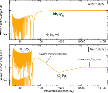
Figure 7: Modulus of the two components $\phi_{g}(r)$ and $\phi_{e}(r)$ of the pair wave function in the FOC approximation, as a function of the interatomic distance. Note that a logarithmic scale is used on both axes. Upper graph: before applying the laser: only ground state pairs exist, $\phi_{e}(r)=0$; the wave function $\phi_{g}(r)$ corresponds to a zero-energy scattering state: it oscillates in the short distance region, where the potential $U_{g}(r)$ is not negligible; for distances $r>$1000 $a_{0}$, the amplitude is equal to the initial condensate density $\rho_{0}$. Lower graph: after applying a cw laser of intensity $I$= 10 kW/cm² during 40 $\mu$s, a level of the excited potential has been populated: $\phi_{e}(r)$ oscillates up to the classical turning point of this level; the population transfer to this excited state is visible in the decrease of both the short-range amplitude of $\phi_{g}(r)$, and its very long-range amplitude corresponding to the condensate density. Note that a strong maximum emerges around $r\sim 55$a₀; it is the near-resonance signature of a weakly bound state in the ground-state channel. At large distances, $\phi_{g}(r)$ shows oscillations, interpreted as outward motion of “hot” correlated pairs ($T\sim$ 4 to 40 $\mu$K).

These two effects arise from the dynamic correlation $\Phi_{g}^{dyn}$ discussed in section IV, but have different interpretations.

VI.3.1 Creation of correlated pairs

Let us first study how the non-condensate atoms are produced. This can be done by analysing the ground state component of the pair wave function, illustrated in Fig. 7. We see that a strong maximum emerges in the wave function $\Phi_{g}$ around 55 a₀, which we identify with the presence of weakly bound molecules, corresponding to population of the last vibrational levels in the X ${}^{1}\Sigma_{g}^{+}$ potential. However, these bound states give a very small contribution to the fraction of non-condensate atoms and they disappear when the laser is turned off. They are in fact a near-resonance feature of the adiabatic correlation $\Phi_{g}^{ad}$ which is already explained by the stationary two-body theory.

The significant fraction of non-condensate atoms is explained by the appearance of waves in the pair wave function at larger distances (Fig. 7). In both FOC and RPW calculation, these waves are created at short distances as soon as the laser is turned on and then propagate in the outward direction, reaching distances where they are no longer affected by the laser coupling -they are not affected when the laser is switched off. This explains why the fraction of non-condensate atoms becomes mostly constant after 5 ${\mu}$s. Thus, these non-condensate atoms correspond to correlated pairs of free atoms with opposite momenta. Their typical kinetic energy is expected to be of the order of $\hbar\Gamma\sim 2\,\mu K$, which is consistent with the wave length of the waves observed in the pair wave function. For weak trapping potentials, they may leave the system. Otherwise, one should treat the collisions between these correlated pairs and the condensate atoms in the presence of the laser field. However this goes beyond both the FOC and RPW approximations.

The appearance of the correlated pairs at high intensity has already been predicted in T. Gasenzer’s work and it was shown that it leads to a saturation of the number of possible stable molecules formed by spontaneous emission Gasenzer (2004). However, it is worth noting that the formation of these pairs is a consequence of the fast rise ($T$=0.5 $\mu$s) of the laser intensity, and is most probably related to a two-body non-adiabatic effect - the waves also appear in a time-dependent two-body calculation. The right column of Fig. 6 shows the on-resonance dynamics when the laser intensity is rised more slowly for $T=16$ $\mu$s. We can see that the final fraction of non-condensate atoms is notably reduced in both approximations. This shows that the creation of correlated pairs is greatly sensitive to the way the laser is turned on. In contrast, the depletion of the condensate still shows a marked deviation from the mean-field prediction. We can then proceed with the discussion of this depletion, ignoring the non-condensate atoms.

VI.3.2 Limitation of the decay rate

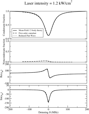
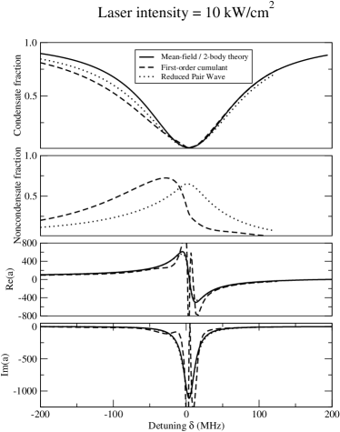
Figure 8: Photoassociation line shape and optical Feshbach resonance: condensate, non-condensate fractions and mean-field scattering length after 40 $\mu s$, as a function of the laser detuning $\delta$ from the bare molecular state (see Fig. 1). At high intensity (10 kW/cm²), the first-order cumulant equations predict highly asymmetric behaviours with respect to the resonance.

In all models, the decay rate of the condensate $K(t)=\frac{h}{m}4|\Im{[a_{M}(t)]}|$ is proportional to the imaginary part of the mean-field scattering length, the latter being one fourth of the photoassociation characteristic length introduced in Ref. McKenzie et al. (2002). The imaginary part of the mean-field scattering is plotted in the bottom panels of Fig. 6. At short times, both the FOC and RPW approximations lead to the same rate, which is clearly smaller than the one predicted by the mean-field approximation. Such a limitation of the rate was already pointed out in the coherent regime Javanainen and Mackie (2002), and also observed in the adiabatic regime Gasenzer (2004).

Our interpretation is the following: because of the rogue dissociation, excited molecules are coupled back to the condensate through the dynamic correlation. This extra correlation reduces the efficiency of the coupling between the condensate and the excited molecules, thereby reducing the loss from the condensate. The fact that this effect does not depend on the way the laser is turned on suggests that it is a genuine many-body effect, namely the influence of the dynamics of the medium on the pair dynamics. We also note that the dynamic correlation responsible for this limitation of the rate gives a very small contribution to the non-condensate atoms, unlike the part corresponding to the correlated free atoms. We suspect from Eqs. (71-75) that the Fourier transform of this correlation scales as $1/k^{4}$.

Note that at longer times in the reduced pair wave approximation, the rate (and more generally the mean-field scattering length) approaches the standard two-body rate (standard scattering length $A$). On the other hand, in the first-order cumulant approximation the rate finally exceeds the standard rate and starts oscillating. However, these differences are not so significant from the experimental point of view because they occur at a point where there are very few condensate atoms remaining in the system.

VI.3.3 Symmetry of the line shape

The differences between the RPW anf FOC approximations are more conspicuous in the line shape of the resonance - see right column of Fig. 8. In the RPW approximation the final condensate and non-condensate fractions are symmetric with respect to the resonance. On the other hand, in the FOC approximation the line shape becomes very asymmetric: on the “blue” side of the resonance (where the bare resonant state lies below the dressed threshold) the condensate is more depleted and more non-condensate atoms are produced than on the “red” side. We suspect that this asymmetry is due to the strong dependence of the scattering properties on the mean-field energy in the FOC approximation, as we saw in Section II.4.2. Indeed, at high-intensity the mean-field energy becomes large and positive on the blue side while it is large and negative on the red side. On the other hand, the scattering properties in the RPW approximation correspond mainly to those of the usual zero energy scattering problem.

Comparison of these predictions with experiment may not be straightforward. First, there are important experimental issues such as inhomogeneous broadenening to overcome at these high intensities McKenzie et al. (2002). Second, collisions between condensate and non-condensate atoms are neglected in both approximations, and as we already pointed out in Section II.5, the RPW approximation brings some correction to the FOC approximation, but only in an incomplete way. However, at a qualitative level, the symmetry of the experimental line shapes at these high intensities could show the relevance of this mean-field correction occurring at short interatomic distance.

VI.3.4 Realistic potentials and cw lasers

Finally, we should note that our calculations using the FOC approximation with realistic potentials agree with T. Gasenzer’s calculations which use a separable potential Gasenzer (2004), except for times when the condensate fraction becomes negligible. This shows that no major improvement is brought by the details of the potential in these cw laser photoassociation calculations. Using the simplified equations (71-75) in this case would lead to similar results. In fact, since we have addressed only the adiabatic regime (see Fig. 2), only two equations would be sufficient, namely (71) and (74) or (71) and (75), as the molecular condensate $\Psi_{m}$can be eliminated adiabatically in these equations. Note that these equations are very similar to those of say, Ref. Javanainen and Mackie (2002), but are free of any ultraviolet divergence or renormalization process as the adiabatic correlation have been eliminated from the equations in the first place.

In the more complex photoassociation processes involving pulsed lasers, the simplified equations are inadequate and we shall use the more general equations and numerical procedures described in this paper to investigate these situations.

VII Conclusion

We have compared two many-body approximations for the time-dependent description of photoassociation and optically-induced Feshbach resonances in an atomic condensate: the first-order cumulant approximation and the reduced pair wave approximation. These approximations differ only in the way the influence of the mean field on a pair of condensate atoms is treated at short separations. Each approximation leads to a set of coupled equations describing the microscopic and macroscopic dynamics for a two-channel problem. We demonstrated that these equations can be solved numerically with realistic molecular potentials, which should prove essential when addressing experiments with chirped laser pulses, for which details of the interaction potentials may influence the dynamics.

From the general equations, we identified several regimes. We define the adiabatic regime when the excited molecular channel is just an intermediate state during the collision of two condensate atoms. In contrast, we define the coherent regime when the excited channel gives rise to a molecular condensate having the features of a one-body condensate. In each of these two regimes, a mean-field theory is obtained when the pair correlation in the ground channel can be eliminated adiabatically. In the coherent regime, this leads to two coupled Gross-Pitaevskiĭ equations Timmermans et al. (1999). In the adiabatic regime, this leads to a single Gross-Pitaevskiĭ equation with a complex scattering length predicted by two-body theories. This is the usual regime investigated so far experimentally McKenzie et al. (2002); Theis et al. (2004); Winkler et al. (2005).

The condition for the breakdown of the mean-field approximation (or so-called rogue dissociation Javanainen and Mackie (2002)) is different in each regime. We showed that, contrary to previous estimates Javanainen and Mackie (2002); McKenzie et al. (2002), the condition for current experiments are under the adiabatic regime.

Solving the general equations numerically, we investigated the case of a sodium condensate where a photoassociation cw laser is turned on in conditions similar to the experiment of McKenzie et al McKenzie et al. (2002). At high intensities ($\sim$10 kW/cm²), which could not be attained in McKenzie et al. (2002) and where rogue dissociation is expected to occur, we observed the following effects:

1. Ground-state correlated pairs of free atoms are produced. This is agrees with the saturation predicted by T. Gasenzer Gasenzer (2004). The creation of such atom pairs can indeed strongly limit the final yield of ground-state molecules formed by spontaneous decay. However, Ref. Gasenzer (2004) considered only a rapid turn on of the laser. By introducing a slower switching procedure, leading to a more adiabatic behaviour, the present work shows that the production of hot atom pairs may be decreased.

2. The photoassociation rate of the condensate at short times is smaller than the rate predicted in the mean-field approximation. This limitation happens at much lower intensities than the unitary limit of the two-body theory. This effect has already been predicted by J. Javanainen and M. Mackie Javanainen and Mackie (2002) in the coherent regime. We interpret it as the appearance of a dynamic many-body correlation in the condensate.

3. The photoassociation line shape becomes asymmetric in the first-order cumulant approximation, while it remains symmetric in the reduced pair wave approximation.

We think this last point should be a good qualitative effect to experimentally distinguish between the two approximations. Future work will investigate the time dependence of the formation of stable molecules, via two-colour or one-colour experiments with pulsed lasers, using the theoretical and numerical tools developed in the present paper.

Acknowledgements P.N. is very grateful to Eite Tiesinga for his essential remarks on this work. Discussions with Arkady Shanenko, Paul Julienne, Thorsten Köhler, Christiane Koch, Eliane Luc-Koenig, Philippe Pellegrini are gratefully acknowledged as well. This work was performed in the framework of the European Research Training Network “Cold Molecules”, funded by the European Commission under contract HPRN CT 2002 00290. P.N. acknowledges for an invitation in Clarendon Laboratory, Oxford.

VIII Appendix

VIII.1 Definition of the non-commutative cumulants

If $\hat{A}_{1},\;\hat{A}_{2},\>...\hat{A}_{n}$ are $n$ bosonic operators, the $n$-order cumulant $\langle\hat{A}_{1}\hat{A}_{2}...\hat{A}_{n}\rangle^{c}$ is defined recursively as follows Köhler and Burnett (2002):

$$\langle\hat{A}_{1}\rangle = \langle\hat{A}_{1}\rangle^{c}$$

$$\langle\hat{A}_{1}\hat{A}_{2}\rangle = \langle\hat{A}_{1}\rangle^{c}\langle\hat{A}_{2}\rangle^{c}+\langle\hat{A}_{1}\hat{A}_{2}\rangle^{c}$$

$$\langle\hat{A}_{1}\hat{A}_{2}\hat{A}_{3}\rangle = \langle\hat{A}_{1}\rangle^{c}\langle\hat{A}_{2}\rangle^{c}\langle\hat{A}_{3}\rangle^{c}\;+\;\langle\hat{A}_{1}\rangle^{c}\langle\hat{A}_{2}\hat{A}_{3}\rangle^{c}$$

$$+\;\langle\hat{A}_{2}\rangle^{c}\langle\hat{A}_{1}\hat{A}_{3}\rangle^{c}\;+\;\langle\hat{A}_{3}\rangle^{c}\langle\hat{A}_{1}\hat{A}_{2}\rangle^{c}$$

$$+\;\langle\hat{A}_{1}\hat{A}_{2}\hat{A}_{3}\rangle^{c}$$

$$\vdots$$

where $\langle...\rangle$ denotes the quantum average in the many-body states of the system. For an ideal gas, we can check that all cumulants containing more than two bosonic operators are zero, according to Wick’s theorem. For a system close to the ideal gas, the cumulants are non-zero but tend to zero as the order is increased. They are therefore a sort of measure of the deviation from the ideal case.

VIII.2 In-medium effective wave functions

VIII.2.1 General expressions

The in-medium pair wave function approach, as we may call it, was initiated by a series of papers by A. Yu. Cherny and A. A. Shanenko. Its aim is to have a many-body description of the dilute Bose gas which remains valid at short interatomic distances, so that interaction potentials with strong repulsive cores can be treated directly. The authors have mainly addressed the problem of the ground state for a homogeneous system. In Ref. Naidon and Masnou-Seeuws (2003), we have generalized some of their ideas to the inhomogeneous time-dependent case. We will recall here the derivation of the in-medium pair wave functions given in Naidon and Masnou-Seeuws (2003), and will show in addition how three-body wave functions can be constructed out of these pair wave functions. This will lead to the reduced pair wave approximation used in this paper.

The starting point is to consider the reduced density matrices of the the many-boson system. As these matrices are hermitian, they can be diagonalized in a basis of orthogonal eigenvectors, associated with positive eigenvalues. For example, the following one-body, and two-body reduced density matrices can be diagonalized as follows:

$$\langle\hat{\psi}^{\dagger}(\mathbf{x})\hat{\psi}(\mathbf{y})\rangle = \sum_{i}\Psi_{i}^{*}(\mathbf{x})\Psi_{i}(\mathbf{y})$$ (102)

$$\frac{1}{2}\langle\hat{\psi}^{\dagger}(\mathbf{w})\hat{\psi}^{\dagger}(\mathbf{z})\hat{\psi}(\mathbf{x})\hat{\psi}(\mathbf{y})\rangle = \sum_{i}\Phi_{i}^{*}(\mathbf{w,z})\Phi_{i}(\mathbf{x,y})\qquad$$ (103)

where the $\Psi_{i}$ are the eigenvectors of the one-body density matrix, and $\Phi_{i}$ are the eigenvectors of the two-body density matrix. We have normalized these vectors to their respective eigenvalues, which means that $N_{i}=\int d^{3}\mathbf{x}|\Psi_{i}(\mathbf{x})|^{2}$ is the eigenvalue associated with $\Psi_{i}$, and $M_{i}=\int d^{3}\mathbf{y}d^{3}\mathbf{x}|\Phi_{i}(\mathbf{x,y})|^{2}$ is the eigenvalue associated with $\Phi_{i}$. As these eigenvectors have the form of wave functions, we call them effective one-body wave functions and effective pair wave functions. $N_{i}$ is interpreted as the average number of particles of the system in the one-body state $|\Psi_{i}\rangle$, and $M_{i}$ is interpreted as the average number of pairs in the two-body state $|\Phi_{i}\rangle$. We can check that $\sum_{i}N_{i}=N$ and $\sum_{i}M_{i}=\frac{1}{2}N(N-1)$, where $N$ is the total number of particles in the system.

In the case of a condensate, a certain one-body wave function $\Psi_{0}$ has a macroscopic occupation number $N_{0}\gg\sum_{i\neq 0}N_{i}$. In the $U(1)$ symmetry breaking picture, this one-body wave function is identified with the condensate wave function, or order parameter $\langle\hat{\psi}\rangle$. According to the Bogoliubov prescription, the field operator $\hat{\psi}$ can then be decomposed into its average value $\Psi_{0}$ and a remaining fluctuating operator $\hat{\theta}$. Expanding the two-body density matrix (103) with the Bogoliubov prescription, and refactorising the expression, we showed that it can be written:

$$\sum_{i=0}^{\infty}\Phi_{0i}^{*}(\mathbf{w,z})\Phi_{0i}(\mathbf{x,y})$$ (104)

$$+\frac{1}{2}\langle\hat{\theta}^{\dagger}(\mathbf{w})\hat{\theta}^{\dagger}(\mathbf{z})\hat{\theta}(\mathbf{x})\hat{\theta}(\mathbf{y})\rangle-\sum_{i\neq 0}^{\infty}{\Phi^{\prime}}_{0i}^{*}(\mathbf{w,z})\Phi^{\prime}_{0i}(\mathbf{x,y})$$

where:

$$\Phi_{00}(\mathbf{x,y}) = \frac{1}{\sqrt{2}}\Psi_{0}(\mathbf{x})\Psi_{0}(\mathbf{y})\;+\;\Phi_{00}^{\prime}(\mathbf{x,y})$$ (105)

$$\Phi_{0i}(\mathbf{x,y}) = \frac{\Psi_{0}(\mathbf{x})\Psi_{i}(\mathbf{y})+\Psi_{0}(\mathbf{y})\Psi_{i}(\mathbf{x})}{\sqrt{2}}+\Phi_{0i}^{\prime}(\mathbf{x,y})\qquad$$ (106)

for $i\neq 0$ and:

$$\Phi_{00}^{\prime}(\mathbf{x,y}) = \frac{1}{\sqrt{2}}\langle\hat{\theta}(\mathbf{x})\hat{\theta}(\mathbf{x})\rangle$$

$$\Phi_{0i}^{\prime}(\mathbf{x,y}) = \int d^{3}\mathbf{z}\frac{\Psi_{i}(\mathbf{z})}{\sqrt{2N_{i}}}\langle\hat{\theta}^{\dagger}(\mathbf{z})\hat{\theta}(\mathbf{x})\hat{\theta}(\mathbf{y})\rangle\quad\text{for $i\neq 0$}$$

As the $\Phi_{0i}$’s and $\Phi_{00}$ are orthogonal in the limit of large systems, we conclude that we have found the first pair wave functions of the diagonalized form (103).

$\Phi_{00}$ is interpreted as the condensate-condensate wave function, ie the wave function for a pair of particles both coming from the condensed part. It is composed of two terms: an asymptotic term $\frac{1}{\sqrt{2}}\Psi_{0}(\mathbf{x})\Psi_{0}(\mathbf{y})$ corresponding to the free motion of two independent condensate particles, and a scattering term $\Phi_{00}^{\prime}$ corresponding to their correlated motion due to their interaction. Similarly, $\Phi_{0i}$ for $i\neq 0$ is interpreted as the condensate-noncondensate wave function, ie the wave function for two particles, one coming from the condensed part and the other coming from the non-condensed part. It is also composed of an asymptotic term $\frac{\Psi_{0}(\mathbf{x})\Psi_{i}(\mathbf{y})+\Psi_{0}(\mathbf{y})\Psi_{i}(\mathbf{x})}{\sqrt{2}}$ (note the symmetrization) and a scattering term $\Phi_{0i}^{\prime}$. We can check that for a sufficiently large system the norm of $\Phi_{00}$ is $\frac{1}{2}N_{0}^{2}$, the number of condensate pairs, and the norm of $\Phi_{0i}$ is $N_{0}N_{i}$, the number of pairs involving a condensate particle and a non-condensate particle in state $|\Psi_{i}\rangle$. The presence of a condensate therefore implies a condensation of unbound pairs, as $\frac{1}{2}N_{0}^{2}\gg\sum_{i\neq 0}N_{0}N_{i}$.

The last line of Eq. (104) corresponds to the remaining pair wave functions of the system. We have no explicit expression for those, but if we assume that the non-condensate particles form an ideal gas (ie do not interact), we can use Wick’s theorem to express the last line, and check that it is equal to:

$$\sum_{0<i\leq j}\Phi_{ij}^{*}(\mathbf{w,z})\Phi_{ij}(\mathbf{x,y})$$

with:

$$\Phi_{ij}(\mathbf{x,y}) = \Psi_{i}(\mathbf{x})\Psi_{i}(\mathbf{y})$$

$$\Phi_{ij}(\mathbf{x,y}) = \frac{\Psi_{i}(\mathbf{x})\Psi_{j}(\mathbf{y})+\Psi_{i}(\mathbf{y})\Psi_{j}(\mathbf{x})}{\sqrt{2}}\quad\text{for }i\neq j$$

which are indeed the expected pair wave functions for two non-interacting non-condensate atoms .

For convenience, we may rewrite the scattering terms appearing in (107) and (108) with multiplicative correlation functions $\varphi_{0i}$ defined as follows:

$$\Phi_{00}(\mathbf{x,y}) \equiv \frac{1}{\sqrt{2}}\Psi_{0}(\mathbf{x})\Psi_{0}(\mathbf{y})\varphi_{00}(\mathbf{x,y})$$ (107)

$$\Phi_{0i}(\mathbf{x,y}) \equiv \frac{\Psi_{0}(\mathbf{x})\Psi_{i}(\mathbf{y})+\Psi_{0}(\mathbf{y})\Psi_{i}(\mathbf{x})}{\sqrt{2}}\varphi_{0i}(\mathbf{x,y})\qquad$$ (108)

Figure 9: Schematic reprensentations of some effective in-medium wave functions in a condensate: the condensate pair wave function $(a)$, the condensate-noncondensate pair wave function $(b)$, the condensate three-body wave function $(c)$, and the condensate-condensate-noncondensate three-body wave function $(d)$. The circles indicate the asymptotic one-body behaviours, and the dashed lines represent the correlation.

We call these functions $\varphi_{0i}$ the reduced pair wave functions. Assuming that the particles must be decorrelated at large distances, we expect that the reduced pair wave functionstend to 1 at large distances. Thus, we may write $\varphi_{0i}=1+\varphi_{0i}^{\prime}$ for convenience, with $\varphi_{0i}^{\prime}$ vanishing at large distances. Another important property is that for an interaction with a strong repulsive core, the probability of finding two particles close to each other should tend to zero at short distances; we therefore expect that the reduced pair wave functions$\varphi_{0i}$ tend to zero at short distances. This is precisely because they tend to zero at short distances that they have a regularising effect when multiplied with the interaction potential.

We can now express the quantum averages found in Eqs. (9) and (14) in terms of pair wave functions. By expanding the quantum average in Eq. (9) with the Bogoliubov prescription and refactorising the terms, we find:

$$\langle\hat{\psi}^{\dagger}(\textbf{z})\hat{\psi}(\textbf{z})\hat{\psi}(\mathbf{x})\rangle=\sqrt{2}\sum_{i=0}^{\infty}\Psi_{i}^{*}(\mathbf{z})\Phi_{0i}(\mathbf{z,x})$$ (109)

This gives a clear interpretation of this term in Eq. (9): the condensate particles can collide either with another condensate particle or with a non-condensate particle. Each type of collision gives rise to a term looking like a scattering amplitude, where the corresponding two-body wave function is involved.

Similarly, by expanding the quantum average in Eq. (14) in terms of cumulants, and refactorising the terms, we find:

$$\langle\hat{\psi}^{\dagger}(\textbf{z})\hat{\psi}(\textbf{z})\hat{\psi}(\mathbf{x})\hat{\psi}(\mathbf{y})\rangle=\sqrt{3!}\sum_{i=0}^{\infty}\Psi_{i}^{*}(\mathbf{z})\Omega_{00i}(\mathbf{z,x,y})$$ (110)

with the three-body wave functions:

$$\Omega_{000}(\mathbf{z,x,y}) \equiv \;\frac{1}{\sqrt{3!}}\Psi_{0}(\!\mathbf{z}\!)\Psi_{0}(\!\mathbf{x}\!)\Psi_{0}(\!\mathbf{y}\!)\>\Big{(}1+{\varphi^{\prime}}_{00}(\mathbf{z,\!x})+{\varphi^{\prime}}_{00}(\mathbf{z,\!y})+{\varphi^{\prime}}_{00}(\mathbf{x,\!y})\Big{)}\;+\;\Omega_{000}^{\prime}(\mathbf{z,x,y})$$

$$\Omega_{00i}(\mathbf{z,x,y}) \equiv \;\frac{1}{\sqrt{3!}}\left(\begin{array}[]{c}\quad\Psi_{i}(\!\mathbf{z}\!)\Psi_{0}(\!\mathbf{x}\!)\Psi_{0}(\mathbf{y})\>\Big{(}1+\varphi_{0i}^{\prime}(\mathbf{z,\!x})+\varphi_{0i}^{\prime}(\mathbf{z,\!y})+\varphi_{00}^{\prime}(\mathbf{x,\!y})\Big{)}\\ +\;\Psi_{i}(\!\mathbf{y}\!)\Psi_{0}(\!\mathbf{z}\!)\Psi_{0}(\mathbf{x})\>\Big{(}1+\varphi_{00}^{\prime}(\mathbf{z,\!x})+\varphi_{0i}^{\prime}(\mathbf{z,\!y})+\varphi_{0i}^{\prime}(\mathbf{x,\!y})\Big{)}\\ +\;\Psi_{i}(\!\mathbf{x}\!)\Psi_{0}(\!\mathbf{z}\!)\Psi_{0}(\mathbf{y})\>\Big{(}1+\varphi_{0i}^{\prime}(\mathbf{z,\!x})+\varphi_{00}^{\prime}(\mathbf{z,\!y})+\varphi_{0i}^{\prime}(\mathbf{x,\!y})\Big{)}\end{array}\right)\;+\;\Omega_{00i}^{\prime}(\mathbf{z,x,y})$$

where:

$$\Omega^{\prime}_{000}(\mathbf{z,x,y}) = \frac{1}{\sqrt{3!}}\langle\hat{\theta}(\mathbf{z})\hat{\theta}(\mathbf{x})\hat{\theta}(\mathbf{y})\rangle^{c}$$

$$\Omega^{\prime}_{00i}(\mathbf{z,x,y}) = \int\!\!d^{3}\mathbf{w}\frac{\Psi_{i}(\mathbf{w})}{\sqrt{3!}N_{i}}\langle\hat{\theta}^{\dagger}(\mathbf{w})\hat{\theta}(\mathbf{z})\hat{\theta}(\mathbf{x})\hat{\theta}(\mathbf{y})\rangle^{c}$$

We note that the first term of each three-body wave functions is not the wave function of independent particles, contrary to what we found with pair wave functions. Indeed, it already contains some pair correlation through the terms $\varphi^{\prime}$. However, these pair correlations are not complete. For an interaction with a strong repulsive core, the probability for finding three atoms very close to one another must tend to zero. But here, the first term of each three-body wave function does not vanish when $\mathbf{x}\approx\mathbf{y}\approx\mathbf{z}$. We think this is because this first term is only the asymptotic behaviour of the three-body wave function at large distances. The terms $\Omega^{\prime}$ must contain stronger correlations at short distances. We expect that at short distances, the three-body wave functions are in fact fully correlated through a product of reduced pair wave functions akin to a Jastrow wave functionJastrow (1955):

$$\Omega_{000}(\mathbf{z,x,y}) \equiv \;\frac{1}{\sqrt{3!}}\Psi_{0}(\!\mathbf{z}\!)\Psi_{0}(\!\mathbf{x}\!)\Psi_{0}(\!\mathbf{y}\!)\>{\varphi}_{00}(\mathbf{z,\!x}){\varphi}_{00}(\mathbf{z,\!y}){\varphi}_{00}(\mathbf{x,\!y})\;+\;\Omega_{000}^{\prime\prime}(\mathbf{z,x,y})$$

$$\Omega_{00i}(\mathbf{z,x,y}) \equiv \;\frac{1}{\sqrt{3!}}\left(\begin{array}[]{c}\quad\Psi_{i}(\!\mathbf{z}\!)\Psi_{0}(\!\mathbf{x}\!)\Psi_{0}(\mathbf{y})\>{\varphi}_{0i}(\mathbf{z,\!x}){\varphi}_{0i}(\mathbf{z,\!y}){\varphi}_{00}(\mathbf{x,\!y})\\ +\;\Psi_{i}(\!\mathbf{y}\!)\Psi_{0}(\!\mathbf{z}\!)\Psi_{0}(\mathbf{x})\>{\varphi}_{00}(\mathbf{z,\!x}){\varphi}_{0i}(\mathbf{z,\!y}){\varphi}_{0i}(\mathbf{x,\!y})\\ +\;\Psi_{i}(\!\mathbf{x}\!)\Psi_{0}(\!\mathbf{z}\!)\Psi_{0}(\mathbf{y})\>{\varphi}_{0i}(\mathbf{z,\!x}){\varphi}_{00}(\mathbf{z,\!y}){\varphi}_{0i}(\mathbf{x,\!y})\end{array}\right)\;+\;\Omega_{00i}^{\prime\prime}(\mathbf{z,x,y})$$

This is the most natural structure which preserves the symmetry of the three-body wave functions and leads to a zero probability at short distances. The remaining terms $\Omega^{\prime\prime}$ are supposed to contain the three-body correlations which cannot be expressed in terms of two-body correlations. Note again that the norm of $\Omega_{000}$ is $\frac{1}{3!}N_{0}^{3}$ corresponding to the number of condensate triplets, while the norm of $\Omega_{00i}$ is $\frac{1}{2}N_{0}^{2}N_{i}$, corresponding to the number of triplets involving two condensate particles and one particle in the non-condensate state $|\Psi_{i}\rangle$.

The interpretation of (110) appearing in Eq. (14) is again very simple: the pairs of condensate atoms can collide either with another condensate atom, or with a non-condensate atom. Each type of collision is accounted for by a scattering amplitude-like term, involving the corresponding three-body wave function.

VIII.2.2 Simplified expressions

Neglecting the collisions with non-condensate particles as well as the three-body correlation $\Omega_{000}^{\prime\prime}$, we can express the quantum averages in terms of only the condensate wave function $\Psi\equiv\Psi_{0}$ and the condensate pair wave function $\Phi=\sqrt{2}\Phi_{00}$:

$$\langle\hat{\psi}^{\dagger}(\textbf{w})\hat{\psi}(\textbf{z})\hat{\psi}(\mathbf{x})\rangle \approx \Psi^{*}(\mathbf{w})\Phi(\mathbf{z,x})$$ (113)

$$\langle\hat{\psi}^{\dagger}(\mathbf{w})\hat{\psi}^{\dagger}(\mathbf{z})\hat{\psi}(\mathbf{x})\hat{\psi}(\mathbf{y})\rangle \approx \Phi^{*}(\mathbf{w,z})\Phi(\mathbf{x,y})$$ (114)

$$\langle\hat{\psi}^{\dagger}(\textbf{w})\hat{\psi}(\textbf{z})\hat{\psi}(\mathbf{x})\hat{\psi}(\mathbf{y})\rangle \approx \Psi^{*}(\mathbf{w})\frac{\Phi(\mathbf{z,x})\Phi(\mathbf{z,y})\Phi(\mathbf{x,y})}{\Psi(\mathbf{x})\Psi(\mathbf{y})\Psi(\mathbf{z})}\qquad$$ (115)

Note that all these expressions respect the symmetry of the quantum averages by exchange of coordinates. Approximations (113) and (114) are found within the first-order cumulant approach, but not Approximation (115). The reduced pair wave approximation (27) used in this paper is a simplified version of (115) where the correlation between $\mathbf{z}$ and $\mathbf{x}$ is neglected.

References

- Sauer et al. (1994) B. E. Sauer, J. Wang, and E. A. Hinds, Bull. Am. Phys. Soc. Ser. H. 39, 1060 (1994).
- E.A.Hinds (1997) E.A.Hinds, Physica Scripta T70, 34 (1997).
- Heinzen et al. (2000) D. J. Heinzen, R. Wynar, P. D. Drummond, and K. V. Kheruntsyan, Phys. Rev. Lett. 84, 5029 (2000).
- Donley et al. (2002) E. A. Donley, N. R. Claussen, S. T. Thompson, and C. E. Wieman, Nature 417, 529 (2002).
- Claussen et al. (2002) N. Claussen, E. Donley, S. Thompson, and C. Wieman, Phys. Rev. Lett. 89, 010401 (2002).
- Herbig et al. (2003) J. Herbig, T. Kraemer, M. Mark, T. Weber, C. Chin, H.-C. Nägerl, and R. Grimm, Science 301, 1510 (2003).
- Xu et al. (2003) K. Xu, T. Mukaiyama, J. R. Abo-Shaeer, J. K. Chin, D. E. Miller, and W. Ketterle, Phys. Rev. Lett. 91, 210402 (2003).
- Dürr et al. (2004) S. Dürr, T. Volz, A. Marte, and G. Rempe, Phys. Rev. Lett. 92, 020406 (2004).
- Regal et al. (2003) C. A. Regal, C. Ticknor, J. L. Bohn, and D. S. Jin, Nature 424, 47 (2003).
- Zwierlein et al. (2003) M. W. Zwierlein, C. A. Stan, C. H. Schunck, S. M. F. Raupach, S. Gupta, Z. Hadzibabic, and W. Ketterle, Phys. Rev. Lett. 91, 250401 (2003).
- Strecker et al. (2003) K. E. Strecker, G. B. Partridge, and R. G. Hulet, Phys. Rev. Lett. 91, 080406 (2003).
- Cubizolles et al. (2003) J. Cubizolles, T. Bourdel, S. Kokkelmans, G. Shlyapnikov, and C. Salomon, Phys. Rev. Lett. 91, 240401 (2003).
- Jochim et al. (2003a) S. Jochim, M. Bartenstein, A. Altmeyer, G. Hendl, C. Chin, J. H. Denschlag, and R. Grimm, Phys. Rev. Lett. 91, 240402 (2003a).
- Jochim et al. (2003b) S. Jochim, M. Bartenstein, A. Altmeyer, G. Hendl, S. Riedl, C. Chin, J. H. Denschlag, and R. Grimm, Science 302, 2101 (2003b).
- Regal et al. (2004) C. A. Regal, M. Greiner, and D. S. Jin, Phys. Rev. Lett. 92, 040403 (2004).
- Fedichev et al. (1996) P. O. Fedichev, Y. Kagan, G. V. Shlyapnikov, and J. T. M.Walraven, Phys. Rev. Lett. 77, 2913 (1996).
- Bohn and Julienne (1997) J. L. Bohn and P. S. Julienne, Phys. Rev. A 56, 1486 (1997).
- Kokoouline et al. (2001) V. Kokoouline, J. Vala, and R. Kosloff, J. Chem. Phys. 114, 3046 (2001).
- Fatemi et al. (2000) F. Fatemi, K. Jones, and P. Lett, Phys. Rev. Lett. 85, 4462 (2000).
- Theis et al. (2004) M. Theis, G. Thalhammer, K. Winkler, M. Hellwig, G. Ruff, R. Grimm, and J. H. Denschlag, Phys. Rev. Lett. 93, 123001 (2004).
- Thalhammer et al. (2005) G. Thalhammer, M. Theis, K. Winkler, R. Grimm, and J. H. Denschlag, Phys. Rev. A 71, 033403 (2005).
- Koch et al. (2005) C. P. Koch, F. Masnou-Seeuws, and R. Kosloff, Phys. Rev. Lett. 94, 193001 (2005).
- Koch et al. (2004) C. P. Koch, J. P. Palao, R. Kosloff, and F. Masnou-Seeuws, Phys. Rev. A 70, 013402 (2004).
- Drummond and Kheruntsyan (1998) P. Drummond and K. Kheruntsyan, Phys. Rev. Lett. 81, 3055 (1998).
- Timmermans et al. (1999) E. Timmermans, P. Tommasini, M. Hussein, and A. Kerman, Phys. Rep. 315 (1999).
- Vardi et al. (2001) A. Vardi, V. A. Yurovksi, and J. Anglin, Phys. Rev. A 64, 063611 (2001).
- Kokkelmans and Holland (2002) S. J. J. M. F. Kokkelmans and M. J. Holland, Phys. Rev. Lett. 89, 180401 (2002).
- Mackie et al. (2002) M. Mackie, K.-A. Suominen, and J. Javanainen, Phys. Rev. Lett. 89, 180403 (2002).
- Köhler et al. (2003) T. Köhler, T. Gasenzer, P. S. Julienne, and K. Burnett, Phys. Rev. Lett. 91, 230401 (2003).
- Drummond and Kheruntsyan (2004) P. Drummond and K. Kheruntsyan, Phys. Rev. A 70, 033609 (2004).
- Vala et al. (2001) J. Vala, O. Dulieu, F. Masnou-Seeuws, and R. Kosloff, Phys. Rev. A 63, 013412 (2001).
- Luc-Koenig et al. (2004a) E. Luc-Koenig, R. Kosloff, F. Masnou-Seeuws, and M. Vatasescu, Phys. Rev. A 70, 033414 (2004a).
- Luc-Koenig et al. (2004b) E. Luc-Koenig, M. Vatasescu, and F. Masnou-Seeuws, Eur. Phys. J. D 31, 239 (2004b).
- Köhler and Burnett (2002) T. Köhler and K. Burnett, Phys. Rev. A 65, 033601 (2002).
- Köhler et al. (2003) T. Köhler, T. Gasenzer, and K. Burnett, Phys. Rev. A 67, 013601 (2003).
- Góral et al. (2004) K. Góral, T. Köhler, T. Gasenzer, and K. Burnett, J. Mod. Opt. 51, 1731 (2004).
- Fricke (1996) J. Fricke, Ann. Phys. 252, 479 (1996).
- Naidon and Masnou-Seeuws (2003) P. Naidon and F. Masnou-Seeuws, Phys. Rev. A 68, 033612 (2003).
- Cherny and Shanenko (2000) A. Y. Cherny and A. A. Shanenko, Phys. Rev. E 62, 1646 (2000).
- Cherny and Shanenko (2002) A. Y. Cherny and A. A. Shanenko, Phys. Lett. A 293, 287 (2002).
- McKenzie et al. (2002) C. McKenzie, J. H. Denschlag, H. Häffner, A. Browaeys, L. E. de Araujo, F. Fatemi, K. M. Jones, J. Simsaran, D. Cho, A. Simoni, et al., Phys. Rev. Lett. 88, 120403 (2002).
- Pitaevskiĭ and Stringari (2003) L. Pitaevskiĭ and S. Stringari, Bose-Einstein Condensation (Oxford University Press, 2003).
- Leggett (2001) A. J. Leggett, Rev. Mod. Phys. 73, 307 (2001).
- Lee et al. (1957) T. D. Lee, K. Huang, and C. N. Yang, Phys. Rev. 106, 1135 (1957).
- Kokkelmans et al. (2002) S. Kokkelmans, J. Milstein, M. Chiofalo, R. Walser, and M. Holland, Phys. Rev. A 65, 053617 (2002).
- Jastrow (1955) R. Jastrow, Phys. Rev. 98, 1479 (1955).
- Yukalov (1990) V. I. Yukalov, Phys. Lett. A 42, 3324 (1990).
- Leggett (2003) A. J. Leggett, New Journal of Physics 5, 103.1 (2003).
- Cherny and Brand (2004) A. Y. Cherny and J. Brand, Phys. Rev. A 70, 043622 (2004).
- Gasenzer (2004) T. Gasenzer, Phys. Rev. A 70, 021603(R) (2004).
- Allen and Eberly (1987) L. Allen and J. Eberly, Optical resonance and two-level atoms (Dover, New York, 1987).
- Fioretti et al. (1998) A. Fioretti, D. Comparat, A. Crubellier, O. Dulieu, F.Masnou-Seeuws, and P. Pillet, Phys. Rev. Lett. 80, 4402 (1998).
- Masnou-Seeuws and Pillet (2001) F. Masnou-Seeuws and P. Pillet, Adv. At. Mol. Opt. Phys 47, 53 (2001).
- Javanainen and Mackie (2002) J. Javanainen and M. Mackie, Phys. Rev. Lett. 88, 090403 (2002).
- Winkler et al. (2005) K. Winkler, G. Thalhammer, M. Theis, H. Ritsch, R. Grimm, and J. H. Denschlag, Phys. Rev. Lett. 95, 063202 (2005).
- Kokoouline et al. (1999) V. Kokoouline, O. Dulieu, R. Kosloff, and F. Masnou-Seeuws, J. Chem. Phys. 110, 9865 (1999).
- Press et al. (1996) W. H. Press, S. A. Teukolsky, W. T. Vettering, and B. P. Flannery, Numerical recipes (2nd edition) (Cambride University Press, 1996), www.nr.com.
- Pellegrini (2003) P. Pellegrini, Ph.D. thesis (2003).
- Marinescu and Dalgarno (1995) M. Marinescu and A. Dalgarno, Phys. Rev. A 52, 311 (1995).