Scattering functions of knotted ring polymers

Abstract

We discuss the scattering function of a Gaussian random polygon with $N$ nodes under a given topological constraint through simulation. We obtain the Kratky plot of a Gaussian polygon of $N=200$ having a fixed knot for some different knots such as the trivial, trefoil and figure-eight knots. We find that some characteristic properties of the different Kratky plots are consistent with the distinct values of the mean square radius of gyration for Gaussian polygons with the different knots.

I Introduction

Ring polymers have attracted much interest in polymer physics, and various properties have been studied both theoretically and experimentally. Casassa ; Vologodskii ; Roovers ; Semlyen ; Burchard ; tenBrinke For the Gaussian random polygon the analytic expression of the static structure factor was obtained by Casassa. Casassa The Kratky plot of the scattering function is compared with that of star polymers with four or five arms. Casassa ; Burchard The scattering data of cyclic polystyrene in deuteriated cyclohexane was obtained by the SANS experiment. tenBrinke

Recently statistical properties of ring polymers under topological constraints have been investigated extensively mainly through computer simulation. desCloizeaux-Let ; Deutsch ; GrosbergPRL ; Miyuki ; Akos ; Matsuda ; Moore ; PRE2001R ; PRE-Miyuki It is first conjectured by des Cloizeaux that a topological constraint should lead to an effective repulsion among segments of ring polymers desCloizeaux-Let . The conjecture is supported by the numerical observations that the mean square radius of gyration of ring polymers with a fixed knot is larger than that of no topological constraint. Deutsch ; Miyuki ; Akos ; Matsuda ; Moore ; PRE2001R ; PRE-Miyuki In fact, the topological swelling is observed particularly for ring polymers with small or zero excluded volume. PRE2001R ; PRE-Miyuki

In this paper we discuss the scattering function of ring polymers under a topological constraint. It should be fundamental for studying ring polymers in scattering experiments. We consider ring polymers in solution at the $\theta$ temperature, and they are modeled by random polygons. Here, random polygons have no excluded volume, i.e. they have no thickness. We shall evaluate the radial distribution function in simulation, and then take the Fourier transformation. We shall show the Kratky plot of the scattering function of a random polygon having some fixed knot type.

II Simulation Methods

Making use of the conditional probability distribution desCloizeaux-Mehta , we have systematically constructed $10^{5}$ samples of the Gaussian random polygon with $200$ nodes. We have calculated two knot invariants, $\Delta_{K}(-1)$ and $v_{2}(K)$, to each of the $10^{5}$ configurations, and effectively classified them into different topological classes. Here the symbol $\Delta_{K}(-1)$ denotes the determinant of a knot $K$, which is given by the Alexander polynomial $\Delta(t)$ evaluated at $t=-1$. The symbol $v_{2}(K)$ is the Vassiliev invariant of the second degree. We select such polygons that have the same set of values of the two knot invariants. Here we calculate $v_{2}(K)$ by the algorithm Polyak . The two knot invariants are practically useful for computer simulation of random polygons with a large number of polygonal nodes DeguchiPLA .

We consider four different topological classes: the trivial knot ($0$), the trefoil knot ($3_{1}$), the figure-eight knot ($4_{1}$) and the other knots ($other$), in the paper. We denote by “$all$” such polygons that have no topological constraint.

Let us denote by $\langle R_{G,K}^{2}\rangle$ the mean square radius of gyration for such Gaussian polygons that have $N$ nodes and a given topological constraint $K$. The estimates of $\langle R_{G,K}^{2}\rangle$ for $N=200$ are given in Table 1 for several knots. For different numbers of $N$, they have been obtained in Ref. Miyuki, . The fraction of Gaussian polygons with a given knot has also been evaluated for some knots. Tsurusaki

$K$	$\langle R_{G,K}^{2}\rangle$	errors
$0$	18.033	0.082
$3_{1}$	16.208	0.120
$4_{1}$	15.043	0.250
$other$	13.459	0.118
$all$	16.674	0.060

Table 1: Mean square radius of gyration $\langle R_{G,K}^{2}\rangle$ of a Gaussian random polygon with a topological condition $K$. Here $N=200$.

Figure 1: The probability distribution $4\pi r^{2}\,g_{K}(r)\Delta r/N$ versus the distance $r$. Here $N=200$ and $\Delta r=0.1$. The plots of the five topological conditions, $all$, $0$, $3_{1}$, $4_{1}$ and $other$, are represented by crosses, tilted crosses, double crosses, open squares and open circles, respectively.

III Radial distribution functions

Let us define the segment pair correlation function of a random polygon with $N$ nodes by Doi

$$g({\bm{r}})={\frac{1}{N}}\sum_{m,n=1}^{N}\langle\delta({\bm{r}}-({\bm{R}}_{m}-{\bm{R}}_{n}))\rangle\,.$$ (1)

Here ${\bm{R}}_{m}$ denotes the position vector of the $m$th node for $m=1,2,\ldots,N$. Due to spherical symmetry, the function $g({\bm{r}})$ depends only on the distance, $r=|{\bm{r}}|$, and we denote it by $g(r)$. We call it the radial distribution function. Here we note that $4\pi r^{2}g(r)\Delta r/N$ gives the probability of other segments appearing in a spherical shell from radius $r$ to $r+\Delta r$ centered at a given segment.

For a Gaussian polygon under a topological condition $K$, we denote by $g_{K}({\bm{r}})$ and $g_{K}(r)$ the pair correlation function and the radial distribution function, respectively. The graphs of the probability distribution $4\pi r^{2}g_{K}(r)\Delta r/N$ are plotted against $r$ in Fig. 1. They are consistent with a preliminary result proceedings .

We now generalize the recent observation that for random polygons the peak position of the probability distribution $4\pi r^{2}g(r)\Delta/N$ should be given by the gyration radius. Kamata Let us denote by $R_{G,K}$ the square root of the mean-square radius of gyration, i.e. $R_{G,K}=\sqrt{\langle R_{G,K}^{2}\rangle}$. The estimates of the peak position of the probability distribution $4\pi r^{2}g_{K}(r)\Delta r/N$ for the five topological conditions are listed in Table 2 together with those of the gyration radius, $R_{G,K}$. They are almost identical up to numerical errors. Thus, we have $r_{\rm peak}=R_{G,K}$ within errors. This is characteristic to ring polymers. In fact, for a Gaussian linear chain, the peak position of the probability distribution $4\pi r^{2}g(r)\Delta r/N$ is located at $r\approx 0.74R_{G,lin}$, where $R_{G,lin}$ denotes the square root of the mean square radius of gyration for the linear chain. Teraoka

$K$	$r_{\rm peak}$	$R_{G,K}$
$0$	4.25	4.246
$3_{1}$	4.05	4.026
$4_{1}$	3.85	3.879
$other$	3.65	3.669
$all$	4.05	4.083

Table 2: Peak position $r_{\rm peak}$ of the probability distribution $4\pi r^{2}g_{K}(r)\Delta r/N$ for a topological condition $K$. The estimates of $r_{\rm peak}$ may have errors of order 0.1 at most.

IV Scattering functions

For a random polygon with $N$ nodes, we define the (single-chain) static structure factor $g({\bm{q}})$ by the Fourier transform of the pair correlation function as follows Doi

$$g({\bm{q}})=\int d{\bm{r}}e^{i{\bm{q}}\cdot{\bm{r}}}g({\bm{r}})={\frac{1}{N}}\sum_{m,n=1}^{N}\langle\exp(i{\bm{q}}\cdot({\bm{R}}_{m}-{\bm{R}}_{n}))\rangle$$ (2)

We also call it the scattering function. The scattering function $g({\bm{q}})$ depends only on $q=|{\bm{q}}|$, and we denote it by $g(q)$. For a Gaussian polygon under a topological condition $K$, we denote the static structure factor or the scattering function by the symbol $g_{K}(q)$.

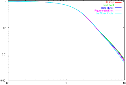
Figure 2: Double logarithmic plot of the form factor $P_{K}(q)$ of an $N$-noded Gaussian polygon under a topological condition $K$ versus the variable $u=qR_{G,K}$. The curves colored with red, green, blue, magenta, and cyan correspond to the cases of $all$, $0$, $3_{1}$, $4_{1}$ and $other$, respectively.

Let us introduce the form factor $P_{K}(q)$ for a Gaussian polygon under a topological condition $K$ as follows

$$P_{K}(q)={\frac{g_{K}(q)}{g_{K}(0)}}$$ (3)

We have $P_{K}(q)=g_{K}(q)/N$ from (2). We have evaluated the form factor $P_{K}(q)$ for the five topological conditions. Let us define variable $u$ by $u=qR_{G,K}$. The double logarithmic plot of the form factor $P_{K}(q)$ versus $u$ is shown in Fig. 2. Here we recall that the form factor $P_{all}(q)$ was evaluated analytically in terms of the Dawson integral. Casassa

In the region from $u=0$ up to $u=2$ or 3, the form factors $P_{K}(q)$ for the five topological conditions overlap each other. For $u>5$, the graphs of the different topological conditions make parallel lines. The gradient is almost given by $-2$, which is consistent with the Gaussian asymptotic behavior.

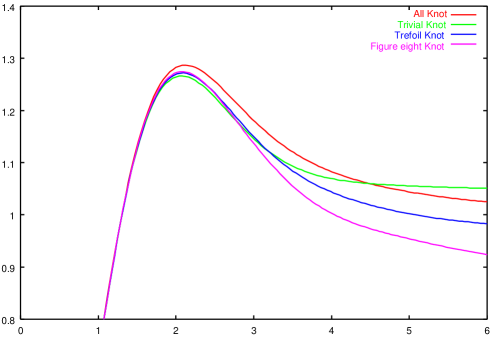
Figure 3: Plot of $(qR_{G,K})^{2}\,P_{K}(q)$ versus $u=qR_{G,K}$. The Kratky plots of the trivial, trefoil and figure-eight knots are represented by the green, blue and magenta curves, respectively. The red curve corresponds to the case of no topological constraint.

Let us discuss the Kratky plots of the form factors $P_{K}(q)$ for some different topological conditions. The plots of $(qR_{G,K})^{2}P_{K}(q)$ versus the variable $u=qR_{G,K}$ are shown in Fig. 3. Here we have numerically evaluated the Fourier transformations of the radial distribution functions by an interpolation method Kamata .

$K$	$u_{\rm peak}$	peak height
$0$	2.08	1.266
$3_{1}$	2.09	1.272
$4_{1}$	2.09	1.275
$other$	2.09	1.300
$all$	2.08	1.287

Table 3: Peak position $u_{\rm peak}$ of the Kratky plot $(qR_{G,K})^{2}\,P_{K}(q)$ versus $u=qR_{G,K}$ for the Gaussian random polygon under a given topological condition $K$. The $q$ value is given by an integral multiple of $0.01$.

For the graphs shown in Fig. 3 we observe that the mean square radius of gyration, $\langle R_{G,K}^{2}\rangle$, plays a central role in the scattering function of the Gaussian polygon under a topological condition, $K$. In the small $u$ region such as $u<2$, the plots for the different topological conditions overlap completely, while for $u>2$ the graphs become separate. Here, the peak positions of the Kratky plots are given by the same value of $u$ for all the five topological conditions. The estimates of the peak positions are given in Table 3. The peak height depends on topological conditions. The Kratky plot for the trivial knot has the smallest peak height. The peak height for the trefoil knot is a little larger than that of the trivial knot. However, for the Kratky plots of the trefoil and figure-eight knots, the peak heights are given by almost the same value.

The Kratky plots of Fig. 3 are not in contradiction with those of previous studies, and even generalize them. For lattice random polygons with $N=160$, the Kratky plots were numerically evaluated for all polygons and knotted polygons, respectively. tenBrinke Since the majority of polygons with nontrivial knots for $N=200$ are given by those of the trefoil knot, the Kratky plots of all polygons and knotted polygons in Ref. tenBrinke, approximately correspond to those of no topological constraint and the trefoil knot shown in Fig. 3, respectively.

For $u>5$, we observe that each of the Kratky plots of Fig. 3 approach constant values. We thus suggest an asymptotic behavior that for any topological constraint $K$ the form factor $P_{K}(q)$ should become close to that of the Gaussian polygon for $u\gg 1$, such as $P_{K}(q)\propto 1/(qR_{G,all})^{2}$. Here we recall that when $u\gg 1$ the form factor $P_{lin}(q)$ of a Gaussian linear chain is approximated by $P_{lin}(q)\approx 2/(q^{2}{R^{2}_{G,lin}})$. We thus have

$$(qR_{G,K})^{2}\,P_{K}(q)\propto{\frac{R_{G,K}^{2}}{R_{G,all}^{2}}}\quad(u\gg 1)$$ (4)

The asymptotic constant value of the Kratky plot of a knot $K$ should become smaller when the knot $K$ becomes more complex. It is consistent with the observation of Fig. 3 that the order of the asymptotic constant values are the same with that of the values $\langle R_{G,K}^{2}\rangle$ in Table 1, for the three knots. For $u>10$, systematic errors of the Kratky plots may be larger than statistical errors of the gyration radius $R_{G,K}$.

The distribution function between two given nodes of a random polygon with a fixed knot is recently evaluated through simulation, and it is found to be close to the Gaussian one. Yao The interpretation (4) should be also consistent with the observation.

V Conclusion

We have evaluated the scattering functions of Gaussian random polygons with $N=200$ under different topological conditions $K$. The Kratky plots have been obtained for the different $K$. They overlap up to $u=2$, and they become separate for $u>2$, and they approach constant values for $u\gg 1$. Several characteristic properties are explained in terms of the different values of the gyration radius $R_{G,K}$.

References

- (1) E. F. Casassa, J. Polym. Sci., Part A 3, 605 (1965).
- (2) A.V. Vologodskii, A.V. Lukashin, M.D. Frank-Kamenetskii, and V.V. Anshelevich, Sov. Phys. JETP 39, 1059 (1974).
- (3) J. R. Roovers and P. M. Toporowski, Macromolecules 16, 843 (1983).
- (4) Cyclic Polymers, ed. J.A. Semlyen (Elsevier Applied Science Publishers, London and New York, 1986); 2nd Edition (Kluwer Academic Publ., Dordrecht, 2000).
- (5) W. Burchard, in Cyclic Polymers, ed. J.A. Semlyen (Elsevier Applied Science Publishers, London and New York, 1986) pp. 43–84.
- (6) G. ten Brinke and G. Hadziioannou, Macromolecules 20, 480 (1987).
- (7) J. des Cloizeaux, J. Physique Letters (France) 42 , L433 (1981).
- (8) J. M. Deutsch, Phys. Rev. E 59, R2539 (1999).
- (9) A. Yu. Grosberg, Phys. Rev. Lett. 85, 3858 (2000).
- (10) M. K. Shimamura and T. Deguchi, J. Phys. A: Math. Gen. 35, L241 (2002).
- (11) A. Dobay, J. Dubochet, K. Millett, P. E. Sottas and A. Stasiak, Proc. Natl. Acad. Sci. USA 100, 5611 (2003).
- (12) H. Matsuda, A. Yao, H. Tsukahara, T. Deguchi, K. Furuta and T. Inami, Phys. Rev. E 68, 011102 (2003).
- (13) N. T. Moore, R. C. Lua and A. Y. Grosberg, Proc. Natl. Acad. Sci. USA 101, 13431 (2004).
- (14) M. K. Shimamura, and T. Deguchi, Phys. Rev. E 64, 020801(R) (2001)
- (15) M. K. Shimamura and T. Deguchi, Phys. Rev. E 65, 051802 (2002).
- (16) J. des Cloizeaux and M. L. Mehta, J. Phys. (Paris) , 665 (1979).
- (17) M. Polyak and O. Viro, Int. Math. Res. Not. No.11, 445 (1994).
- (18) T. Deguchi and K. Tsurusaki, Phys. Lett. A 174, 29 (1993).
- (19) T. Deguchi and K. Tsurusaki, Phys. Rev. E. 55, 6245 (1997) .
- (20) M. Doi, Introduction to Polymer Physics (Clarendon Press, Oxford, 1996)
- (21) M. K. Shimamura and T. Deguchi, preprint.
- (22) I. Teraoka, Polymer Solutions (John Wiley Sons, Inc., New York, 2002).
- (23) K. Kamata, Scattering functions of circular polymers (in Japanese), Master thesis, Ochanomizu University, March 2005.
- (24) A. Yao, H. Tsukahara, T. Deguchi and T. Inami, J. Phys. A: Math. Gen. 37, 7993 (2004).