Bound states in Andreev billiards with soft walls

Abstract

The energy spectrum and the eigenstates of a rectangular quantum dot containing soft potential walls in contact with a superconductor are calculated by solving the Bogoliubov-de Gennes (BdG) equation. We compare the quantum mechanical solutions with a semiclassical analysis using a Bohr–Sommerfeld (BS) quantization of periodic orbits. We propose a simple extension of the BS approximation which is well suited to describe Andreev billiards with parabolic potential walls. The underlying classical periodic electron-hole orbits are directly identified in terms of “scar” like features engraved in the quantum wavefunctions of Andreev states determined here for the first time.

I Introduction

The interface between a normal-conducting (N), ballistic quantum dot and a superconductor (S) gives rise to the coherent scattering of electrons into holes.Blonder et al. (1982) This phenomenon, which is of great experimental Morpurgo et al. (1997); Pothier et al. (1994); Charlat et al. (1996) and theoretical Lambert and Raimondi (1998); Bagwell (1992); Stone (1996); Beenakker (1997); Kosztin et al. (1995); Wiersig (2002); Duncan and Györffy (2002); Mortensen et al. (1999); Cserti et al. (2000) interest, is generally known as Andreev reflection.Andreev (1964) A N-S hybrid structure consisting of a superconductor attached to a normal cavity is commonly called an Andreev billiard. For a recent and comprehensive review of these systems see, e.g., Ref. Beenakker, 2004 and references therein.

An important quantity for Andreev billiards is the density of states (DOS) which has been studied theoretically by many authors.Melsen et al. (1996); Lodder and Nazarov (1998); Adagideli and Goldbart (2002); Cserti et al. (2004a, 2002a, 2002b); Kormányos et al. (2003, 2004); Cserti et al. (2004b) Its behavior close to the Fermi energy depends on the classical dynamics found in the isolated normal conducting cavity: In the integrable case, the DOS is proportional to the energy, while for a classically chaotic normal cavity, a minigap (which is smaller than the bulk superconductor gap $\Delta_{0}$) develops. Moreover, depending on the geometry of the normal cavity one can observe singularities in the DOS. A well-known example of such a behavior of the DOS is an Andreev billiard formed from a normal metal film attached to a superconductor studied long ago by de Gennes and Saint-James.de Gennes and Saint-James (1963) Recently, similar singular features of the DOS have been found in other Andreev billiards.Cserti et al. (2002a, b); Kormányos et al. (2003); Koltai et al. (2004); Cserti et al. (2004b)

To calculate the DOS for Andreev billiards many researchers have successfully applied the Bohr–Sommerfeld (BS) approximation.Melsen et al. (1996); Lodder and Nazarov (1998); Adagideli and Goldbart (2002); Schomerus and Beenakker (1999); Ihra et al. (2001); Cserti et al. (2004a, 2002a, 2002b); Kormányos et al. (2003); Koltai et al. (2004); Cserti et al. (2004b); Beenakker (2004) It was shown that the DOS can be related to the purely geometry-dependent path length distribution $P(l)$ which is the classical probability that an electron entering the N region at the N-S interface returns to the interface after a path length $l$.

In the present work, we discuss on the one hand quantum and semiclassical results for Andreev billiards with walls which are mediating a smooth transition between the interior of the cavity and the region outside. On the other hand, we calculate, for the first time, the wavefunctions of eigenstates in such Andreev billiards. As a prototypical example for an Andreev billiard confined by soft walls, we choose a parabolic wall profile, as shown in Fig. 1. Such soft-walled Andreev billiards are of interest because they describe the potential profile found in studies of typical quantum dots realized by remote surface gates.Bird et al. (1995) Soft walls are a quite realistic approximation which extends previous theoretical work where infinitely high walls were employed. We demonstrate that with suitable adaptions, the BS approximation can describe N-S hybrid systems in which the electrostatic potential in the normal conducting cavity is modelled by a parabolic potential. Recently, Silvestrov et al. Silvestrov et al. (2003) have presented a quasiclassical study of Andreev billiards containing smoothly varying potentials inside the normal dot. However, no exact quantum mechanical calculation of the energy levels of such Andreev billiards has been performed. We succesfully tested the predictions for the DOS obtained from our BS approximation by comparing them to results found from exact quantum mechanical calculations using the Bogoliubov-de Gennes (BdG) equation.

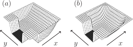
Figure 1: Andreev billiard with parabolic walls at ($a$) the wall opposite to the lead and ($b$) at all sides except the one the superconducting lead is attached to. The superconducting area is shaded.

A better understanding of the BS approximation can be gained by the analysis of electron and hole wavefunctions of Andreev states which we determine by the modular recursive Green’s function method (MRGM).Rotter et al. (2000, 2003) Based on recent theoretical studies Leadbeater and Lambert (1995); Claughton et al. (1995) the wave function patterns observed in Andreev billiards may be scanned by measuring the tunneling conductance of such systems. We show that the wave functions feature enhanced density over continuous families of classical periodic orbits (“bundles”Wirtz et al. (1997)). These bundles of classical orbits give rise to peaks in the pathlength distribution $P(l)$ and, as a consequence, the DOS shows singular behavior at certain energies. Moreover, a close similarity between the electron and the hole components of the eigenstates is observed in line with the semiclassical picture of the Andreev retroreflection process.

This paper is organized as follows. In Sec. II the method for calculating the quantum mechanical eigenenergies and eigenstates is presented along with our extended semiclassical approach. In Sec. III our numerical results are presented. Finally, the paper concludes with a short summary in Sec. IV.

II Methods

In this section we outline our quantum mechanical method for determining the energy levels and the corresponding eigenstates of the N-S hybrid systems shown in Figs. 1($a$) and ($b$). Moreover, we present the semiclassical approach for the density of states.

The normal region of the N-S hybrid system is a ballistic, rectangular cavity. The length of the side of the cavity parallel to the N-S interface is $L$. For the spatial dependence of the confining potential $V(\mathbf{x})$, we consider in this work two cases: i) one parabolic-type soft wall is placed opposite to the N-S interface and all other sides of the rectangle (apart from the N-S interface) are hard walls (see Fig. 1($a$)), i.e.

$$V(\mathbf{x})=\left\{\begin{array}[]{ll}\alpha\,E_{F}(x-x_{0})^{2}\Theta\left(x-x_{0}\right)&\rm{if}\ \ 0\leq y\leq L\\ \infty&\rm{elsewhere}\end{array}\right.$$ (1a)

and ii) three sides of the normal cavity are confined by a parabolic-type soft wall (see Fig. 1($$b V(\mathbf{x})$$)) and hence is given by

$$V(\mathbf{x}) = \alpha E_{\rm{F}}\left[\left(x-x_{0}\right)^{2}\Theta(x-x_{0})+y^{2}\Theta(-y)\right.$$ (1b)

$$\left.+\left(y-L\right)^{2}\Theta(y-L)\right],$$

where in both cases $\alpha$ is a parameter controlling the steepness of the soft wall, $\Theta$ is the Heaviside function, while the parameters $x_{0}$ and $L$ fix the position of the potential. The superconducting region of width $W$ ($W\leq L$) is attached to the remaining side of the cavity. An ideal interface between the normal and the superconducting region is assumed, i.e. the effective masses and the Fermi energies are the same in the N and S regions, and no tunnel barrier is present at the interface.

The superconducting pairing potential $\Delta_{0}$ is constant in the S region and zero in the N region. This approximation is valid if the superconducting coherence length $\xi$ is small compared to the characteristic size of the rectangular cavity.Beenakker (1997) Thus, the pairing potential is given by a step function model $\Delta(\mathbf{x})=|\Delta_{0}|\ \Theta(x_{\rm{NS}}-x)$, where the coordinate system $\mathbf{x}=(x,y)$ is chosen such that the N-S interface is located at $x_{\rm{NS}}=0$.

II.1 Quantum mechanical solution

The quantum mechanical description of the N-S hybrid system is given by the BdG equation de Gennes and Saint-James (1963)

$$\left(\begin{array}[c]{cc}H_{0}&\Delta\\ \Delta^{*}&-H_{0}^{*}\end{array}\right)\left(\begin{array}[c]{c}u(\mathbf{x})\\ v(\mathbf{x})\end{array}\right)=\varepsilon\left(\begin{array}[c]{c}u(\mathbf{x})\\ v(\mathbf{x})\end{array}\right),$$ (2)

where $H_{0}={\bf p}^{2}/(2m^{*})+V(\mathbf{x})-E_{\rm{F}}$ is the single-particle Hamiltonian with the confining potential $V(\mathbf{x})$ that defines the normal dot and $m^{*}$ is the effective mass. The electron and the hole part of the quasiparticle wave function are denoted by $u(\mathbf{x})$ and $v(\mathbf{x})$, respectively, whereas $\varepsilon$ is the excitation energy of the quasiparticle measured from the Fermi energy $E_{\rm{F}}$. In this work we study the bound states of Andreev billiards, i.e. the eigenenergies $\varepsilon$ are in the range $0\leq\varepsilon\leq\Delta$.

The energy levels $\varepsilon_{i}$ of the hybrid system are found by matching the wave functions at the N-S interface. To construct the wave functions satisfying the Bogoliubov-de Gennes equation in the two regions we follow the methods of Beenakker Beenakker (1991, 2004) and Cserti et al.. Cserti et al. (2002b) The wave function in the normal region can be expressed in terms of the scattering matrix $S(\varepsilon)$ of the open system in which the superconductor is replaced by a normal lead. This scattering matrix is calculated by the modular recursive Green’s function method developed by Rotter et al. Rotter et al. (2000, 2003) Note that this method to study Andreev billiards is, within the model assumption outlined above, exact. In particular, it does not rely on the usual Andreev approximation,Blonder et al. (1982) i.e., $\Delta_{0}\ll E_{\rm{F}}$, and the assumption of quasi-particles whose angle of incidence/reflection are approximately perpendicular to the N-S interface.Lambert and Raimondi (1998)

The integrated density of states (in the following called state counting function) can be obtained from the energy levels $\varepsilon_{i}$ as

$$N_{\rm{QM}}(\varepsilon)=\sum_{i}\Theta(\varepsilon-\varepsilon_{i}).$$ (3)

In our numerical calculations discussed below $N_{\rm QM}(\varepsilon)$ can be obtained directly. Therefore, it is straightforward to compare the state counting functions obtained from the exact quantum mechanical calculations with that from the BS approximation. The numerical differentiation to determine the DOS can thus be by-passed.

We now sketch the method for calculating the wave functions in the two regions. From the matching conditions one can find the expansion coefficients $b_{n}^{e}\,,\ b_{n}^{h}$ of the wave functions in the S region, and $c_{n}^{e,\pm}\,,\ c_{n}^{h,\pm}$ in the N region in terms of the right ($+$) and left ($-$) moving plane waves given by

$$\chi_{n}^{\pm}(\mathbf{x};E)=\sqrt{\frac{2m^{*}}{\hbar k_{x,n}W}}\ e^{\pm ixk_{x,n}}\sin(yk_{y,n}),$$ (4)

where $k_{y,n}=n\pi/W$ and $k^{2}_{x,n}=2m^{*}E/\hbar^{2}-k_{y,n}^{2}$ are the transverse and longitudinal wavenumbers respectively, and $W$ is the width of the N-S interface (here the wave functions are flux normalized). The wave function in the S region is given by

$$u_{S}(\mathbf{x}) = \sum_{n}\left[\gamma b_{n}^{e}\chi_{n}^{-}(\mathbf{x};E^{+})+\gamma^{*}b_{n}^{h}\chi_{n}^{+}(\mathbf{x};E^{-})\right]$$ (5a)

$$v_{S}(\mathbf{x}) = \sum_{n}\left[b_{n}^{e}\chi_{n}^{-}(\mathbf{x};E^{+})+b_{n}^{h}\chi_{n}^{+}(\mathbf{x};E^{-})\right],$$ (5b)

where $\gamma=\Delta/(\varepsilon+i\sqrt{\Delta^{2}-\varepsilon^{2}})$, $E^{\pm}=E_{\rm{F}}\pm i\sqrt{\Delta^{2}-\varepsilon^{2}}$, and the asterisk denotes complex conjugation. Note that to ensure the boundary conditions at $x\to-\infty$, only the right (left) moving plane waves $\chi_{n}^{+}(\mathbf{x};E^{-})$ ($\chi_{n}^{-}(\mathbf{x};E^{+})$) enter in the expansion of the wave function in the S region.

Calculation of the wave function in the normal dot requires two steps. At first we obtain the wave function at the N-S interface using the expansion coefficients $c_{n}^{e,\pm}$ and $c_{n}^{h,\pm}$ calculated from the matching conditions at the N-S interface. Secondly, the wave function inside the dot can be written as

$$u_{N}(\mathbf{x},\varepsilon) = \sum_{n}c_{n}^{e,+}\psi_{n}(\mathbf{x},\varepsilon),$$ (6a)

$$v_{N}(\mathbf{x},\varepsilon) = \sum_{n}c_{n}^{h,-}\psi_{n}(\mathbf{x},-\varepsilon),$$ (6b)

where the $\psi_{n}(\mathbf{x},\varepsilon)$ are the scattering wave functions of a particle inside the dot which can be obtained by projecting the retarded Green function $G(\mathbf{x},\mathbf{x}^{\prime},E)$ of the cavity onto the incoming wave:Baranger and Stone (1989)

$$\psi_{n}(\mathbf{x},\varepsilon)=i\hbar\sqrt{v_{x,n}}\int_{0}^{W}\!\!\!\!\!\!\rm{d}y^{\prime}\ G(\mathbf{x},\mathbf{x}^{\prime},E_{\rm{F}}+\varepsilon)\eta_{n}(y^{\prime}),$$ (7)

where $\eta_{n}(y)=\sqrt{2/W}\,\sin\left(\frac{n\pi y}{W}\right)$ and $v_{x,n}=\hbar k_{x,n}/m^{*}$. While the wavefunction in the superconductor is given as a sum of analytically determined functions in the continuum limit, the wavefunction in the normal conductor is determined numerically on a tight-binding grid. In spite of these two very different approaches, we were able to fulfill the matching conditions with remarkable accuracy. The latter is a measure for the degree of convergence of the tight-binding grid calculation towards the continuum limit.

II.2 Semiclassical treatment

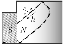
Figure 2: A rectangular Andreev billiard with one parabolic wall defined by Eq. (1a) (darker shading in the N region corresponds to higher potential). One typical Andreev orbit, consisting of an electron part (dashed line) and a hole part (dotted line), is shown.

Over the last decade, the Bohr–Sommerfeld approximation for the smoothed density of states has been successfully applied to Andreev billiards.Melsen et al. (1996); Lodder and Nazarov (1998); Adagideli and Goldbart (2002); Schomerus and Beenakker (1999); Ihra et al. (2001); Cserti et al. (2004a, 2002a, 2002b); Kormányos et al. (2003); Koltai et al. (2004); Cserti et al. (2004b); Beenakker (2004) In the case of a normal dot confined by one N-S interface and infinitely high potential walls, the integrated density of states or smoothed state counting function in the BS approximation reads

$$N_{\rm{BS}}(\varepsilon)=M\sum_{n=0}^{\infty}\int_{l_{n}(\varepsilon)}^{\infty}P(l)dl,$$ (8)

where the integer part of $M=k_{\rm F}W/\pi$ is the number of propagating modes in a lead of width $W$ at the Fermi energy $E_{\rm F}=\hbar^{2}k_{\rm F}^{2}/(2m^{*})$ (here $k_{\rm F}$ is the Fermi wave number) and $P(l)$ denotes the path length distribution, i.e. the classical probability density for electrons entering the billiard at the N-S contact to exit after a path length $l$. Finally, $l_{n}(\varepsilon)$ is given by

$$l_{n}(\varepsilon)=\left[n\pi+\rm{arccos}\left(\frac{\varepsilon}{\Delta}\right)\right]\frac{\hbar v_{\rm{F}}}{\varepsilon},$$ (9)

with $v_{\rm{F}}$ the Fermi velocity. In order to derive Eq. (9), one assumes that the hole retraces the path of the electron (retracing approximation, see Fig. 2). This allows one to quantize the periodic orbits created by two subsequent Andreev reflections using the BS quantization condition for N-S systems:

$$S_{e}-S_{h}=\int_{\Gamma}(\mathbf{p}_{e}-\mathbf{p}_{h})d\mathbf{q}=2\pi\hbar\,(n+\frac{\mu}{4}+\phi).$$ (10)

In Eq. (10) $\mu$ stands for the Maslov index (for details see, e.g., Ref. Brack and Bhaduri, 1997), $\phi=\frac{1}{\pi}\,\arccos(\varepsilon/\Delta)$ represents the energy dependent phase shift resulting from Andreev reflection at the N-S interface and $\Gamma$ is an arbitrary path of geometric length $l_{g}$ connecting one point at the N-S interface with another (see e.g. the one indicated in Fig. 2). The integral in Eq. (10) for a normal dot with hard walls results in $S_{e}-S_{h}=2\varepsilon\,l/v_{\rm{F}}$ from which Eq. (9) follows.

We now extend the BS quantization to soft walls constructed from harmonic potentials. Due to the form of the confining potential $V(\mathbf{x})=V(x)+V(y)$ defined in Eq. (1), the component of the momentum parallel to the soft wall is a constant of motion. Therefore the action (Eq. (10)) for the part of $\Gamma$ which lies in the $V(\mathbf{x})\neq 0$ region can be decomposed as $S_{e}-S_{h}=S_{\parallel}+S_{\perp}$, where $S_{\parallel}$ ($S_{\perp}$) involves the momentum components parallel (${\bf p}_{e,\parallel}-{\bf p}_{h,\parallel}$) and perpendicular (${\bf p}_{e,\perp}-{\bf p}_{h,\perp}$) to the wall. Calculation of $S_{\parallel}$ is trivial since ${\bf p}_{e,\parallel}-{\bf p}_{h,\parallel}$ is constant, resulting in $S_{\parallel}=({\bf p}_{e}-{\bf p}_{h})l_{\parallel}\sin\vartheta$ where $\vartheta$ denotes the angle between ${\bf p}_{e}$ and ${\bf p}_{e,\parallel}$ or between ${\bf p}_{h}$ and ${\bf p}_{h,\parallel}$, while $l_{\parallel}$ corresponds to the displacement parallel to the soft wall which is approached by the particle. $S_{\perp}$ can be evaluated for the parabolic potential (Eq. (1)) as

$$S_{\perp}=\pi\,\sqrt{\frac{2m^{*}}{\alpha E_{\rm{F}}}}\,\varepsilon\cos^{2}\vartheta.$$ (11)

Note that within the retracing approximation the vectors ${\bf p}_{e}$ and ${\bf p}_{h}$ at a given position $\mathbf{x}$ are antiparallel to each other while their magnitude is different for $\varepsilon\neq 0$, i.e. $|{\bf p}_{e}|\neq|{\bf p}_{h}|$. Finally, in Eq. (10), the integration over that part of $\Gamma$ that lies in the potential-free region gives $2\varepsilon\,l/v_{\rm{F}}$, where $l$ represents the path length of the electron travelling in the potential-free region. Putting all these pieces together, the total integral in Eq. (10) can be expressed as $S_{e}-S_{h}=2\varepsilon\,\tilde{l}/v_{\rm{F}}$, where

$$\tilde{l}=l+l_{\parallel}\sin\vartheta+\pi\frac{\cos^{2}\vartheta}{\sqrt{\alpha}}\,.$$ (12)

This result implies that for soft-wall billiards with a confining potential given by Eq. (1), the Bohr–Sommerfeld approximation to the state counting function (Eq. (8)) is still applicable if the classical geometric pathlength distribution $P(l)$ is modified to account for the potential contribution to the action (Eq. (11)). The BS quantization therefore involves a modified pathlength distribution $\tilde{P}(\tilde{l})$. Accordingly, we perform a Monte Carlo simulation with typically $10^{6}$ trajectories, where each trajectory is calculated by a forth-order Runge-Kutta integration. We determine its length $l$ in the potential free region as well as the contribution from the displacement parallel to the soft wall $l_{\parallel}$. Subsequently, $l$ is transformed to $\tilde{l}$ (Eq. (12)) for each encounter with one of the soft walls. Note that the return probability $\tilde{P}(\tilde{l})$ obtained in this way differs from that calculated from the geometric length of the curved trajectories. The effective path length $\tilde{l}$ (Fig. (3)) associated with the action of the particle in the harmonic potential is longer than the geometric length $l_{g}$. The reason for this surprising behavior is that while the individual actions $S_{\perp}^{e}$ and $S_{\perp}^{h}$ of the particle and the hole propagating in the parabolic potential are smaller than $l_{g}\,p_{\perp}^{0}$, with the geometric length $l_{g}$ and the constant momentum $p_{\perp}|_{V=0}=p_{\perp}^{0}$, the difference between the particle and the hole actions $S_{\perp}^{e}-S_{\perp}^{h}$ is larger than $l_{g}(p_{\perp}^{0,e}-p_{\perp}^{0,h})$.

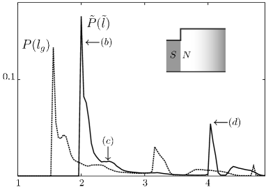
Figure 3: Comparison between the geometric path length distribution $P(l_{g})$ (taking into account the length of the curved trajectories) and the modified path length distribution $\tilde{P}(\tilde{l})$ (Eq. (12)). Both $l_{g}$ and $\tilde{l}$ are given in units of $L$. The inset shows the geometry: Andreev billiard with one parabolic wall, $W=0.7L$, $\alpha=6.7$, $x_{0}=0.4L$. The letters ($b$)-($d$) denote the lengths $\tilde{l}$ of those bundles of classical orbits, at which the wave functions show enhancement in Fig. 4.

III Numerical results

In this section we compare the state counting function obtained from the exact numerical quantum calculations with that predicted by the BS approximation presented above. We consider a ballistic dot confined by ($a$) one or ($b$) three parabolically shaped potential walls as shown in Fig. 1. Moreover, we present both particle as well as hole components of the wavefunction of eigenstates of these N-S hybrid systems.

III.1 One soft wall

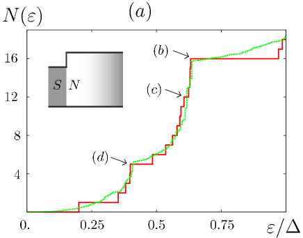
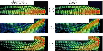
Figure 4: (color online) ($a$) Comparison between the quantum mechanical state counting function $N(\varepsilon)$ (solid red staircase) and the BS prediction, $N_{\rm{BS}}(\varepsilon)$, (Eq. (8), dashed green line) for a N-S system shown in the upper left inset. The modulus square $|u_{N}|^{2}$ and $|v_{N}|^{2}$ (see Eq. (6)) of the three eigenstates marked in ($a$) are shown in ($b$-$d$) to illustrate the correspondence between continuous families of classical trajectories and the quantum mechanical wavefunctions. The parameters are $M=15$, $W=0.7L$, $h=0$, $\alpha=6.7$, $x_{0}=0.4L$ and $\Delta/E_{\rm F}=0.02$.

We first consider an N-S system in which the normal dot is confined by one parabolic potential as shown in Fig. 1($a$). Numerically we have found that most classical trajectories starting from the N-S interface will hit the parabolic wall once, before returning to the superconductor (see e.g. the trajectory indicated in Fig. 2). This feature allows us to test our semiclassical approach on a comparatively simple level before proceeding to the more complicated case of three parabolic walls. We find that the agreement between the exact quantum mechanical calculations for $N_{\rm QM}(\varepsilon)$ and its semiclassical counterpart $N_{BS}(\varepsilon)$ is generally very good (see Fig. 4($a$)), which proves that our semiclassical approach extended to Andreev billiards with soft walls is well suited to describe these systems. A small discrepancy arises only at excitation energies above the cusp marked ($b$) in Fig. 4($a$). We also note, that both curves show a distinct cusp structure, which has also been found in other Andreev billiards. Cserti et al. (2002a, 2000, 2004b) These cusps can be understood from the BS approximation as being the consequence of the behavior of the path length distribution $\tilde{P}(\tilde{l})$ at certain path lengths. For example, as shown in Fig. 3, $\tilde{P}(\tilde{l})$ has a peak at $\tilde{l}=2L$ which results in the most pronounced cusp of the state counting function at $\varepsilon/\Delta=0.63$, as obtained from Eq. (9). This cusp, marked ($b$) in Fig. 4($a$), corresponds to the shortest classical orbits possible in the system. The electron leaves perpendicular to the N-S interface, is reflected back at the soft wall, and then reaches the N-S interface again. Such trajectories are similar to the stationary chords found in Ref. Adagideli and Goldbart, 2002. The corresponding peak in $\tilde{P}(\tilde{l})$ (also marked as ($b$) in Fig. 3) represents a continuous family of trajectories (or bundlesWirtz et al. (1997)) that feature the same topology and bouncing pattern and (almost) the same length, but different initial conditions. In this case, the bundle is generated by a continuous change in the $y$ coordinate at the N-S interface. The corresponding probability density of the wave function in Fig. 4($b$) displays a pronounced enhancement along the bundle of classical periodic orbits. A similar phenomenon has recently been found in pseudointegrable normal billiards Bogomolny and Schmit (2004) and was called superscarring.

According to Eq. (8), for constant quantum number $n$, smaller excitation energies $\varepsilon/\Delta$ correspond to longer classical orbits. This suggests that the excitation energies below the pronounced cusp at $\varepsilon/\Delta=0.63$ correspond to classical orbits with lengths $\tilde{l}>2L$. Indeed, for smaller $\varepsilon/\Delta$ certain wavefunctions mirror bundles of longer classical orbits. Some examples are shown in Fig. 4($c,d$), (see also Fig.  3 for the correspondig path lenghts). The “superscarring” of the corresponding wavefunction near the bundles of short orbits also suggests that the BS approximation reflects the essential features of the underlying quantum dynamics.

III.2 Three soft walls

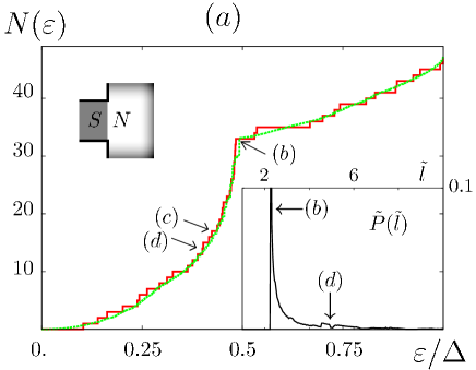
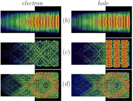
Figure 5: (color online) ($a$) Quantum mechanical state counting function (red solid staircase) and BS approximation (green dashed line) for $\alpha=5.5$. The parameters are $M=30$, $W=L$, $\alpha=125$, $x_{0}=L$ and $\Delta/E_{\rm F}=0.02$. $(b)-(d)$ show selected eigenstates (see text).

We now consider the more complicated case of N-S systems in which the normal dot is confined by three soft walls as shown in Fig. 1($b$).

The agreement between the semiclassical BS approximation (Fig. 5($a$)) and the quantum mechanical calculation for the state counting function is again very good. The position of the cusp in $N_{\rm QM}(\varepsilon)$ can be predicted by the BS approximation to originate from the bundle of shortest trajectories. The corresponding peak in $\tilde{P}(\tilde{l})$ (shown in the lower right inset of Fig. 5($a$)) is located at $\tilde{l}=2.7L$ resulting in a cusp at $\varepsilon/\Delta=0.49$. The wave function of the energy level at the cusp (see Fig. 5($b$)) shows a density enhancement over a bundle of classical periodic orbits analogous to the one discussed for the dot with only one soft wall. As the shortest orbits do not explore the upper and lower horizontal walls, this similarity is to be expected.

Fig. 5($d$) presents projections of an Andreev state that explores the additional soft walls. It mirrors in both the particle and hole components a bundle of classical trajectories all bouncing in sequence at all three soft walls. In line with the retracing approximation, their length $\tilde{l}=3$ is reflected in $\tilde{P}(\tilde{l})$ (marked as ($d$)). The “width” of the bundle (i.e. the continuous range of initial conditions) is, however, narrower than the bundle discussed in the previous paragraph, resulting in a strongly reduced slope in $N_{\rm{BS}}(\varepsilon)$.

A very different scenario emerges for the Andreev eigenstate depicted in Fig. 5($c$). The particle and hole parts display a drastically different pattern pointing to the limitation of the ideal retracing approximation. While the hole part $v_{\rm N}(\mathbf{x})$ is characterized by the “bouncing ball” type scar of trajectories bouncing at the upper and lower horizontal wall, the electron part $u_{\rm N}(\mathbf{x})$ shows no distinct enhancements. Furthermore, integrating $|u_{\rm{N}}(\mathbf{x})|^{2}$ and $|v_{\rm{N}}(\mathbf{x})|^{2}$ over the area of the normal dot we find that the probability of finding the quasiparticle in the hole state is 79% while the probability of the electron state is only 12% (and altogether 9% of finding the quasiparticle in the superconductor). Taking into account also that the hole component $v_{\rm{N}}(\mathbf{x})$ has a very low amplitude at the N-S interface, one can come to the conclusion that the hole part is only weakly coupled to the superconductor. The Andreev state of Fig. 5($c$) can therefore be quantized by assuming that the particle is quasi-bound in the hole space where it spends most of its time with only infrequent and short excursions into the electron space, where it travels on trajectories scattering off the soft walls before returning to the hole space. This observation suggests that for certain individual Andreev states, semiclassical EBK quantization becomes possible, complementing the BS approximation for the smoothed state counting function. The almost vanishing density of $|v_{\rm{N}}|^{2}$ at the N-S interface allows us to assume that the wave function satisfies hard wall boundary conditions along the left wall of the cavity. Accordingly, the eigenenergies are to leading order determined by the quantized actions in the hole space in analogy to long-lived shape resonances. The EBK quantization conditions for the “isolated” hole state therefore read

$$2p_{x}W_{x}+\frac{\pi p_{x}^{2}}{2\sqrt{2m^{*}\alpha E_{F}}} = 2\pi\hbar\left(n+\frac{\mu_{1}}{4}\right)$$ (13a)

$$2p_{y}W_{y}+\frac{\pi p_{y}^{2}}{\sqrt{2m^{*}\alpha E_{F}}} = 2\pi\hbar\left(m+\frac{\mu_{2}}{4}\right)$$ (13b)

where $W_{x}$ and $W_{y}$ are the linear dimensions of the rectangular region where $V=0$, while $p_{x}$ and $p_{y}$ are the $x$ and $y$ components of the momentum of the particle. Here $n$ and $m$ are the quantum numbers characterizing the actions on the tori and $\mu_{1}$ and $\mu_{2}$ are the Maslov indices. The left hand sides of these two equations describe the classical actions corresponding to the motion of the particle along the $x$ (Eq. (13a)) and $y$ (Eq. (13b)) directions.

The Maslov index of $\mu_{1}=3$ in (Eq. (13a)) originates from one reflection at the soft wall and one reflection at the hard wall which replaces the N-S interface, while $\mu_{2}=2$ in Eq. (13b) due to the reflections at the two soft walls. The two equations (13) can be solved for $p_{x}$ and $p_{y}$ as functions of the two quantum numbers $n,m$. The eigenenergy of the N-S system in EBK quantization is then given by $\varepsilon=(p_{x}^{2}+p_{y}^{2})/(2m^{*})-E_{\rm F}$. By inspection of Fig. 5($c$) we find for the hole part of the wave function $|v_{N}|^{2}$ three maxima along the $x$, and 35 along the $y$ direction, respectively. Thus, the two quantum numbers in Eq. (13) are to be taken as $n=2$ and $m=34$, resulting in $|\varepsilon/\Delta|=0.47$. The excitation energy of the state shown in Fig. 5($c$) was found to be $\varepsilon/\Delta=0.448$. This is a remarkable agreement, given that the mean level spacing $\delta_{N}$ of the normal dot in units of $\Delta$ is $0.05$, and taking into account that semiclassical methods usually cannot, to the leading order, resolve the energy spectra on much finer scale than the mean level spacing. The small difference between the energies obtained from the BdG equation and the semiclassical calculation can partly also be attributed to the fact that the wave function at the N-S interface is not exactly zero, i.e., a weak coupling of the normal cavity to the superconductor is present. This result implies that the Andreev state in Fig. 5($c$) is, to a very good approximation, equivalent to an eigenstate of the hole in an isolated cavity. A similar effect of the decoupling of the wave function from the superconductor has been observed in a system of a superconducting disk surrounded concentrically by a normal conductor.Cserti et al. (2002a) In this hybrid system such states were called whispering gallery states.

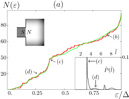
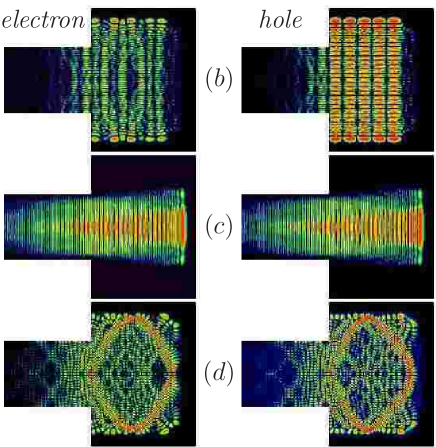
Figure 6: (color online) ($a$) Quantum mechanical state counting function (red solid staircase) and BS approximation (green dashed line) for the same system as in Fig. 5 except for a smaller value of $\alpha=5.5$ (curvature of parabolic wall). $(b)-(d)$ show selected eigenstates (see text).

Finally, we investigate how a smaller $\alpha$, corresponding to a shallower soft wall, affects the agreement with our semiclassical description. We consider the same system as in Fig. 5, only the parabolic slope $\alpha$ (or steepness of the wall) is reduced from $125$ to $5.5$. In such a system, the particle spends more time in the region where $V\neq 0$. The resulting state counting function is shown in Fig. 6($a$). The cusp structure is predicted very accurately by our BS approximation. The most pronounced cusp, marked ($c$) in Fig. 6($a$), is located at an energy of $\varepsilon/\Delta=0.37$. The position of this cusp can again be determined by the peak in the path length distribution $\tilde{P}(\tilde{l})$ at $\tilde{l}=3.3L$, corresponding to the bundle of shortest trajectories. Note, however, that the non-geometric shift in length introduced by Eq. (12) is $1.3L$, and is now comparable to the system size.

The eigenstate shown in Fig. 6($b$) is another example of an Andreev state which, in a very good approximation, corresponds to a bound state of the normal conducting billiard. The hole wavefunction shows 5 maxima in $x$, and 50 maxima in $y$ direction. Inserting $n=4$, $m=49$ into Eq. (13) yields an energy of $|\varepsilon/\Delta|=0.84$. The exact energy of the eigenstate shown in Fig. 6($b$) is $\varepsilon/\Delta=0.86$, while the mean level spacing of the normal dot for this system is $\delta_{N}/\Delta=0.026$. Note that the mean level spacing is changed as compared to the previous case where $\alpha=125$, because the classically allowed area entering into the expression of the mean level spacing of a two dimensional dot is increased.

IV Conclusions

We investigate an Andreev billiard system with harmonic potential walls. A quantum mechanical approach using the BdG equation is presented to calculate the density of Andreev states, and their wave functions for both the electron and hole component. We develop a semiclassical Bohr–Sommerfeld approximation for the smoothed state counting function of a soft-walled Andreev billiard. The quantum mechanical wavefunctions show scar-like density enhancements which correspond to bundles of semiclassical Andreev orbits. Additionally, we find states which feature very different wavefunctions for electron and hole. These states can be understood as quasi-bound states of the electron or hole component of the normal conducting cavity. Their eigenenergies can be determined, in a very good approximation, by using an EBK quantization, assuming hard wall boundary conditions at the N-S interface.