Dynamical scaling in Ising and vector spin glasses

Abstract

We have studied numerically the dynamics of spin glasses with Ising and $XY$ symmetry (gauge glass) in space dimensions 2, 3, and 4. The nonequilibrium spin-glass susceptibility $\chi_{\rm ne}(t_{\rm w},T)$ and the nonequilibrium energy per spin $e_{\rm ne}(t_{\rm w},T)$ of samples of large size $L_{\rm b}$ are measured as a function of anneal time $t_{\rm w}$ after a quench to temperatures $T$. The two observables are compared to the equilibrium spin-glass susceptibility $\chi_{\rm eq}(L,T)$ and the equilibrium energy $e_{\rm eq}(L,T)$, respectively, measured as functions of temperature $T$ and system size $L$ for a range of system sizes. For any time and temperature a nonequilibrium time-dependent length scale $L^{*}(t_{\rm w},T)$ can be defined by writing $\chi_{\rm ne}(t_{\rm w},T)=\chi_{\rm eq}(L^{*},T)$ (or the equivalent expression for the energy). Our analysis shows that for all systems studied, an “effective dynamical critical exponent” parametrization $L^{*}(t_{\rm w},T)=A(T)t^{1/z(T)}$ fits the data well at each temperature within the whole temperature range studied, which extends from well above the critical temperature $T_{\rm c}$ to near $T=0$ for dimension 2 or to well below $T_{\rm c}$ for the other space dimensions studied. In addition, the data suggest that the dynamical exponent $z$ varies smoothly when crossing the transition temperature.

I Introduction

The dynamics of laboratory spin glasses manifests a number of fascinating phenomena, linked to the fact that below the glass temperature $T_{\rm c}$ the systems never achieve true thermodynamic equilibrium.Binder and Young (1986); Young (1998) It has gradually become clear that a slow increase of the coherence length (also known as “dynamic correlation length”) with time plays an important role in the memory and rejuvenation effects seen experimentally in spin glasses under various cooling and heating protocols.Dupuis et al. (2001); Bouchaud et al. (2003); Jönsson et al. (2002a); Bert et al. (2004); Jimenez et al. (2004); Berthier and Young (2005)

Numerical work can also bring light to bear on the question. Finite-size scaling theory states that the dependence of the equilibrium spin-glass susceptibility $\chi_{\rm eq}$ on the system size $L$ at the critical temperature $T_{\rm c}$ is given by

$$\chi_{\rm eq}(L)\sim L^{2-\eta}\;\;\;\;\;\;\;\;\;(T=T_{\rm c}),$$ (1)

where $\eta$ is the “anomalous dimension” static scaling exponent for the correlation function of the system. In addition, at $T_{\rm c}$, the equilibrium autocorrelation relaxation time increases with sample size $L$ as

$$\tau(L)\sim L^{z_{\rm c}}\;,$$ (2)

where $z_{\rm c}$ is the dynamical critical exponent, as conventionally defined for the standard single-spin Glauber update dynamics. HuseHuse (1989) remarked that the critical anneal-time dependence of the nonequilibrium spin-glass susceptibility for large samples after a quench to $T_{\rm c}$ is

$$\chi_{\rm ne}(t_{\rm w})\sim t_{\rm w}^{(2-\eta)/z_{\rm c}}\;,$$ (3)

where $t_{\rm w}$ is the time after quench and $z_{\rm c}$ is again the equilibrium dynamical critical exponent. Equation (3) is strictly equivalent to the definition of an effective time-dependent length scale via

$$L^{*}(t_{\rm w})=A_{\rm c}t_{\rm w}^{1/z_{\rm c}}\;,$$ (4)

with $A_{\rm c}$ an appropriate prefactor. The fact that the nonequilibrium scaling should depend only on the equilibrium dynamical critical exponent $z_{\rm c}$ is important and nontrivial. In the first case the system is quenched from infinite temperature; thus its effective temperature is changing with time all through the annealing process. In the second case $z_{\rm c}$ represents the dynamical scaling for thermal fluctuations within the set of configurations at thermodynamic equilibrium. A rigorous theoretical justification for the nonequilibrium approach exactly at criticality has been given by Jannsen et al.Jannsen et al. (1989) Nonequilibrium dynamics has been studied numerically in considerable detail for many regular magnetic systems,com (a) principally because such data can give accurate information on the critical behavior (see, for instance, Ref. Zheng et al., 1999).

Spin-glass critical nonequilibrium behavior has already been studied numerically in a number of Ising spin glasses (ISG’s) and the gauge glass (GG).Huse (1989); Blundell et al. (1992); Mari and Campbell (2002); Bernardi and Campbell (1997); Katzgraber and Campbell (2004) Relaxation becomes very slow below $T_{\rm c}$ in glassy systems; the phrase “time is length” has been coined for the link between coherence length $\ell(t_{\rm w})$ and anneal time $t_{\rm w}$,Berthier and Bouchaud (2002) and the fact has been underlined that the physically relevant length scales involved in the dynamics of spin glasses below $T_{\rm c}$ are short, even for experimental times which are always very long compared to microscopic time scales. This is because the values of $z_{\rm c}$ in spin glasses are intrinsically high, as the mean field $z_{\rm c}$ at the ISG upper critical dimension $d=6$ is already equal to $4$, and $z_{\rm c}(d)$ increases to yet higher values at lower dimensions.

In numerical simulations of ISG’s below $T_{\rm c}$ the time dependence of the dynamical correlation length $\ell(t_{\rm w})$ has been estimatedParisi et al. (1996); Kisker et al. (1996); Berthier and Bouchaud (2002); Yoshino et al. (2002) by measuring the time-dependent correlation function explicitly and parametrizing using an appropriate assumption for the form of the function. Early correlation length data were analyzed using the phenomenological assumption that a dynamical scaling relationship of the critical functional form, Eq. (4), continues to hold for $\ell(t_{\rm w})$ at temperatures below $T_{\rm c}$, with a temperature-dependent effective dynamical exponent $z(T)$.Kisker et al. (1996); Parisi et al. (1996) It has been suggested that $z(T)\propto 1/T$.Parisi et al. (1996)

Alternatively a “dynamic droplet scaling” has been proposed, where below $T_{\rm c}$ an excitation barrier increases algebraically with correlation length.Fisher and Huse (1988, 1988) For ISG’s in three and four dimensions the consequences of an analysis based on this approach have been discussed in detail in Refs. Berthier and Bouchaud, 2002, Kisker et al., 1996, and Yoshino et al., 2002. This form of parametrization has been widely employed in analyses of experimental dataMattsson et al. (1995); Dupuis et al. (2001); Bouchaud et al. (2001); Jönsson et al. (2002b); Bert et al. (2004) although it should be noted that length scales are never measured directly in experiments.

In the paramagnetic state ($T>T_{\rm c}$), relaxation is fast compared with the time scales of most experiments; therefore measurements of relaxation rates are very difficult. No numerical studies of dynamical length scales seem to have been undertaken either in the regime above the spin-glass freezing temperature in systems having a finite $T_{\rm c}$, except for the two-dimensional (2D) Edwards-Anderson (EA) ISG for which $T_{\rm c}=0$, where careful studies have been undertaken.Kisker et al. (1996); Rieger et al. (2004)

In this work we present results from simulations of the EA ISG with Gaussian-distributed interactions, as well as the GG in dimensions 2, 3, and 4. We choose these models as they are paradigmatic representatives of spin glasses with Ising as well as with vector spin symmetry. We define a temperature-dependent length scale $L^{*}(t_{\rm w},T)$ and find that the equation having the same functional form as Eq. (4) valid at criticality,

$$BL^{*}(t_{\rm w},T)=A(T)t_{\rm w}^{1/z(T)}\;,$$ (5)

with a temperature-dependent effective exponent $z(T)$ and a weakly temperature-dependent prefactor $A(T)$, gives an excellent parametrization of the data in each system, not only at temperatures below $T_{\rm c}$ (confirming the conclusions of Refs. Parisi et al., 1996 and Kisker et al., 1996), but also above $T_{\rm c}$. In addition, we find a disagreement with “droplet dynamic scaling”Berthier and Bouchaud (2002); Yoshino et al. (2002) for the Ising spin glasses, which becomes apparent for temperatures below $\sim T_{\rm c}/2$. For temperatures above $T_{\rm c}$ neither the droplet approach nor the replica symmetry breaking (RSB) approach appears to give any predictions as to a dynamic scaling. For both pictures, “barriers” in the energy landscape disappear above $T_{\rm c}$, therefore relaxation becoming trivial.

In Sec. II we define and discuss a time-dependent length scale which will be needed to rescale the data. In Secs. III and IV we present data for the two-, three-, and four-dimensional gauge glass and Ising spin glass, respectively. After a brief summary (Sec. V), droplet dynamic scaling is discussed in Sec. VI, followed by concluding remarks in Sec. VII.

II Spatiotemporal scaling

The relationship between time and length is defined and discussed below using the internal energy and the spin-glass susceptibility. In general, the internal energy for a spin Hamiltonian is given by

$$e=\frac{1}{N}[\langle{\mathcal{H}}\rangle]_{\rm av}\;.$$ (6)

Here $N=L^{d}$ represents the number of spins described by a Hamiltonian ${\mathcal{H}}$ on a hypercubic lattice of linear size $L$ and $\langle\cdots\rangle$ represents a thermal average, whereas $[\cdots]_{\rm av}$ corresponds to a disorder average.

The spin-glass susceptibility (related to the nonlinear susceptibility measured experimentally) can be expressed as

$$\chi=N[\langle|q|^{2}\rangle]_{\rm av}\;.$$ (7)

Here $q$ represents the Edwards-Anderson order parameter which in the case of the gauge glass is given by

$$q=\frac{1}{N}\sum_{j=1}^{N}\exp[i(\phi_{j}^{\alpha}-\phi_{j}^{\beta})]\;,$$ (8)

with $\phi_{j}$ representing the phases of the $XY$ spins, and $\alpha$ and $\beta$ are two copies of the system with the same disorder. For the Ising spin glass $q$ is given by

$$q={1\over N}\sum_{j=1}^{N}S_{j}^{\alpha}S_{j}^{\beta},$$ (9)

where $S_{j}=\pm 1$ represent Ising spins.

II.1 Definition of a length scale

For any fixed $T$, as the system size $L$ is increased or the anneal time $t_{\rm w}$ lengthed, the SG equilibrium and nonequilibrium susceptibilities $\chi_{\rm eq}(L,T)$ and $\chi_{\rm ne}(t_{\rm w},T)$ grow while the internal equilibrium and nonequilibrium energies per spin, $e_{\rm eq}(L,T)$ and $e_{\rm ne}(t_{\rm w},T)$, respectively, drop towards the infinite-size equilibrium value $e_{\rm eq}(\infty,T)$. If $T$ is above the ordering temperature, $\chi_{\rm eq}(L,T)$ and $\chi_{\rm ne}(t_{\rm w},T)$ will both saturate at a temperature-dependent limiting value $\chi_{\rm eq}(\infty,T)$; $e_{\rm eq}(L,T)$ and $e_{\rm ne}(t_{\rm w},T)$ will always saturate at $e_{\infty}(T)$ for all $T$.

Quite generally, if at any temperature $T$ the equilibrium SG susceptibility as a function of sample size $L$ is $\chi_{\rm eq}(L,T)$ and the nonequilibrium SG susceptibility after an anneal time $t_{\rm w}$ following a quench to temperature $T$ is $\chi_{\rm ne}(t_{\rm w},T)$ for a large sample of size $L_{\rm b}$, then an infinite-sample-size time-dependent length scale $L^{*}(t_{\rm w})$ can be rigorously defined by writing

$$\chi_{\rm eq}[L^{*}(t_{\rm w}),T]=\chi_{\rm ne}(t_{\rm w},T)\;,$$ (10)

as long as $L^{*}(t_{\rm w},T)\ll L_{\rm b}$. This length scale definition applies to any temperature and any anneal time, and the length scale $L^{*}(t_{\rm w},T)$ can be estimated numerically to high precision if data of sufficient statistical accuracy are available. A practical limitation to precision under some conditions is the need to intrapolate between the $\chi_{\rm eq}(L,T)$ sequence of values for integer $L$ to provide a continuous function with which to compare the time-dependent data. In the paramagnetic regime, as $\chi_{\rm eq}(L,T)$ and $\chi_{\rm ne}(t_{\rm w},T)$ both saturate at the equilibrium infinite-size $\chi_{\rm eq}(\infty,T)$ value, $L^{*}(t_{\rm w},T)$ can only be determined up to some temperature-dependent finite time.

An analogous equation can be derived for the energy per spin,

$$e_{\rm eq}[L^{*}(t_{\rm w}),T]=e_{\rm ne}(t_{\rm w},T)\;,$$ (11)

providing an independent estimate for $L^{*}(t_{\rm w},T)$. Later, we show that similar estimates of $L^{*}(t_{\rm w},T)$ are obtained from a completely independent analysis of the data for the susceptibility $\chi$ and energy $e$.

Note that $L^{*}(t_{\rm w},T)$ is not the time-dependent coherence length $\ell(t_{\rm w},T)$,Berthier and Bouchaud (2002) but it is closely related to it. During the anneal each individual spin is surrounded by a growing cohort of spins in equilibrium correlation with it at the temperature $T$, up to a time-dependent cutoff length. This correlated volume can be considered equivalent to a box of linear size $L^{*}(t_{\rm w},T)$. Because $\ell(t_{\rm w},T)$ is defined as a correlation length and $L^{*}(t_{\rm w},T)$ from the box size, we should expect $L^{*}(t_{\rm w},T)\simeq 2\ell(t_{\rm w},T)$. Here, $\ell(t_{\rm w},T)$ has been estimated from directly measured correlation functions, although a fully rigorous definition is not easy to give because of nontrivial prefactors.Kisker et al. (1996); Parisi et al. (1996); Berthier and Bouchaud (2002); Yoshino et al. (2002) For the 3D EA ISG where the comparison can be made directly, the equivalence between $L^{*}(t_{\rm w},T)$ and $2\ell(t_{\rm w},T)$ is indeed found to be correct. It should be borne in mind that because of the disorder, the length values represent averages over different samples and the effective length scale $L^{*}(t_{\rm w},T)$ may be slightly different depending over which observable the mean is being taken.

II.2 Comparison between effective length scales of different observables

There is a straightforward way to test the assumption that the observables $\chi_{\rm ne}(t_{\rm w},T)$ and $e_{\rm ne}(t_{\rm w},T)$ are controlled by a single length scale. At each $T$, the equilibrium energy $e_{\rm eq}(L,T)$ can be written as a function of the equilibrium susceptibility $\chi_{\rm eq}(L,T)$ with $L$ as an implicit parameter: $e_{\rm eq}(L,T)={f}_{e}[\chi_{\rm eq}(L,T)]$. Suppose that Eqs. (10) and  (11) hold, with one and the same $L^{*}(t_{\rm w},T)$ for both observables. Then the nonequilibrium energies $e_{\rm ne}(t_{\rm w},T)$ are given by the identical function ${f}_{e}[\chi_{\rm ne}(t_{\rm w},T)]$ of the nonequilibrium susceptibility $\chi_{\rm ne}(t_{\rm w},T)$, with $t_{\rm w}$ an implicit parameter (see Fig. 1). A plot of nonequilibrium $[e_{\rm ne}(t_{\rm w},T)-e_{\rm eq}(\infty,T)]$ against $\chi_{\rm ne}(t_{\rm w},T)$ data is superimposed on a plot of $[e_{\rm eq}(L,T)-e_{\rm eq}(\infty,T)]$ against $\chi_{\rm eq}(L,T)$ data [by definition the equilibrium and nonequilibrium energy measurements tend to the identical $e_{\rm eq}(\infty,T)$ which we estimate by extrapolation]. These figures are simple displays of raw data, and no fitting procedure whatsoever is involved; at this stage no assumption is made as to the functional form of $L^{*}(t_{\rm w},T)$.

In what follows we present data for the gauge glass, as well as the Ising spin glass.

III Gauge Glass

The gauge glass is a canonical vector spin glass (see, for instance, Refs. Kosterlitz and Akino, 1998; Olson and Young, 2000; Akino and Kosterlitz, 2002) where $XY$ spins on a (hyper)cubic lattice in $d$ dimensions of size $L$ interact through the Hamiltonian

$${\cal H}=-J\sum_{\langle i,j\rangle}\cos(\phi_{i}-\phi_{j}-A_{ij})\;,$$ (12)

the sum ranging over nearest neighbors. The angles $\phi_{i}$ represent the orientations of the $XY$ spins, and the $A_{ij}$ are quenched random variables uniformly distributed between $[0,2\pi]$ with the constraint that $A_{ij}=-A_{ji}$ (here $J=1$). Periodic boundary conditions are applied. The GG ordering temperatures have been shown to be $T_{\rm c}=0$, $0.46(1)$, and $0.89(1)$ in dimensions $2$, $3$, and $4$, respectively.Simkin (1996); Granato (1998); Olson and Young (2000); Katzgraber (2003); Katzgraber and Campbell (2004)

For $XY$ spin systems there is a choice to be made in the allowed single-spin acceptance angle for individual updating steps. To optimize the updating procedure at low temperatures, the limiting angle is often chosen to be less than $2\pi$ for an $XY$ spinKatzgraber and Young (2001) and linearly dependent on temperature. The numerical prefactor for the temperature-dependent window is chosen so that the acceptance ratios for the local Monte Carlo updates is $\sim 0.4$. As far as the final equilibrium parameters are concerned, this choice plays no role. However, for the nonequilibrium simulations it is essential to use the full $2\pi$ acceptance angle window to obtain physically significant results as otherwise the limited angle introduces an artificial temperature variation in the relaxation.

III.1 Two dimensions

The GG in space dimension 2 has a zero-temperature ordering transition.Fisher et al. (1991); Gingras (1992); Reger and Young (1993); Simkin (1996); Granato (1998); Akino and Kosterlitz (2002); Katzgraber and Young (2002); Katzgraber (2003) Therefore all the measurements discussed in this section necessarily refer to the paramagnetic state. Dimension $d=2$ presents the advantage that systems can be equilibrated up to large $L$, so in at least part of the temperature range comparisons can be made between $\chi_{\rm ne}(t_{\rm w},T)$ and $\chi_{\rm eq}(L,T)$ over a wide range of system sizes.com (b) Details of the simulations are presented in the Appendix, Table 2 for equilibrium and Table 8 for nonequilibrium measurements, respectively.

As the systems are always paramagnetic at finite $T$, for the whole temperature range $\chi_{\rm eq}(L)$ must finally saturate at the thermodynamic infinite-size limit and a plot of $\log[\chi_{\rm eq}(L,T)]$ against $\log(L)$ is always curved (although the curvature is weak at small sizes and low $T$). At each temperature a comparison between the nonequilibrium data for the susceptibility $\chi_{\rm ne}(t_{\rm w},T)$ and energy $e_{\rm ne}(t_{\rm w},T)$ and the equilibrium susceptibility $\chi_{\rm eq}(L,T)$ and energy $e_{\rm eq}(L,T)$ can be made. Figures 1–6 show examples at two different temperatures $T=0.173$ and $T=0.513$. In each case a plot is first made of

$$e_{\rm p}(t_{\rm w})=[e_{\rm ne}(t_{\rm w},T)-e_{\rm eq}(\infty,T)]$$ (13)

against $\chi_{\rm ne}(t_{\rm w},T)$ and of

$$e_{\rm p}(L,T)=[e_{\rm eq}(L,T)-e_{\rm eq}(\infty,T)]$$ (14)

against $\chi_{\rm eq}(L,T)$. The excellent superpositions show that to good accuracy the effective length scale $L^{*}(t_{\rm w},T)$ for the two observables is the same throughout the anneal at each temperature. In both equations $e_{\rm eq}(\infty,T)$ is estimated by extrapolation. The evaluation of $L^{*}(t_{\rm w},T)$ from the energy data is not sensitive to $e_{\rm eq}(\infty,T)$ as long as exactly the same value is used for the equilibrium and nonequilibrium data.

To obtain $L^{*}(t_{\rm w},T)$ explicitly, the $\chi_{\rm ne}(t_{\rm w},T)$ data are scaled onto the equilibrium $\chi_{\rm eq}(L,T)$ data, translating to $\chi(L^{*},T)$ by assuming the space-time relation in Eq. (5) and adjusting $A(T)$ and $z(T)$ to obtain optimum scaling. Scaling plots are shown for the same two temperatures. The condition $L^{*}(t_{\rm w},T)\ll L_{\rm b}$ is well satisfied for all the data with the present ranges of sizes and maximum anneal time. At the higher temperatures studied (as in Fig. 4 for $T=0.513$), $\chi_{\rm eq}(L,T)$ and $\chi_{\rm ne}(t_{\rm w},T)$ saturate and the range of points from which the fit is usable is restricted to lengths and times before the onset of saturation. For $T=0.513$ accurate scaling can still be obtained, but this condition leads to a practical upper limit on the temperatures over which $A(T)$ and $z(T)$ can be estimated. Note that these two temperatures are chosen as typical examples of the behavior in the two regimes in which the data sets do not or do arrive at saturation, respectively, within the available ranges of $L$ and $t_{\rm w}$. In other space dimensions and for the Ising systems the equivalent plots always take on one or other of the behaviors depending on the temperature.

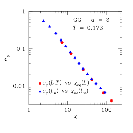
Figure 1: (Color online) Energy difference between the energy per spin for a large sample ($L=128$) at time $t_{\rm w}$ after quench and the infinite time energy, Eq. (13), plotted against the large-sample spin-glass susceptibility after quench $\chi_{\rm ne}(t_{\rm w})$ (triangles) for the two-dimensional GG at $T=0.173$. On the same plot the equilibrium energy difference for size $L$ [Eq. (14)] is plotted against the equilibrium susceptibility $\chi_{\rm eq}(L)$ for the same size (squares). These are raw data, and no fitting is involved in these plots.

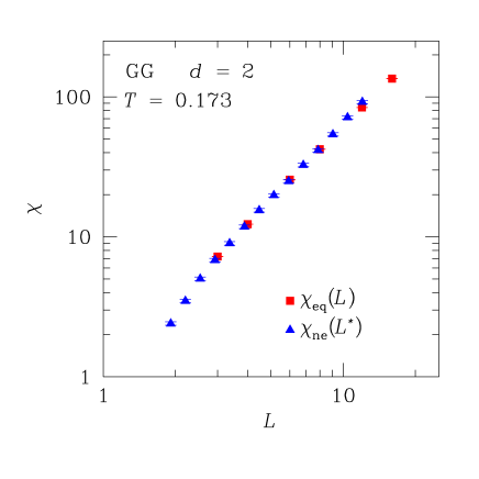
Figure 2: (Color online) Finite-size equilibrium susceptibilities $\chi_{\rm eq}(L)$ vs $L$ (squares) for the two-dimensional GG at $T=0.173$. In addition, the susceptibilities $\chi_{\rm ne}(t_{\rm w})$ at time $t_{\rm w}$ after a quench are plotted against $L^{*}(t_{\rm w})=A(t_{\rm w})t_{\rm w}^{1/z(T)}$ with the parameters $A$ and $z$, both temperature dependent, adjusted for optimal overall overlap with the equilibrium data points (triangles). In this figure $L^{*}(t_{\rm w})=1.66t_{\rm w}^{1/4.9}$.

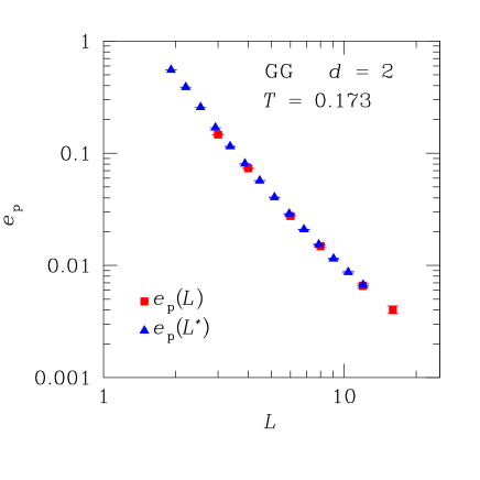
Figure 3: (Color online) Finite-size equilibrium energy differences $e_{\rm p}(L)$ [Eq. (14)] vs $L$ (squares) for the two-dimensional GG at $T=0.173$. On the same plot the energy differences $e_{\rm p}(t_{\rm w})$ at time $t_{\rm w}$ [Eq. (13)] after a quench are plotted against $L^{*}(t_{\rm w})=A(t_{\rm w})t_{\rm w}^{1/z(T)}$ with identical parameters $A(T)$ and $z(T)$ as used in Fig. 2 (triangles). In this figure $e_{\rm p}=e+1.502$.

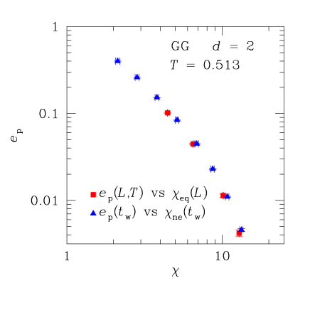
Figure 4: (Color online) Two-dimensional GG equilibrium (squares) and nonequilibrium (triangles) susceptibility and energy data for $T=0.513$, as in Fig. 1. Note the nontrivial functional form.

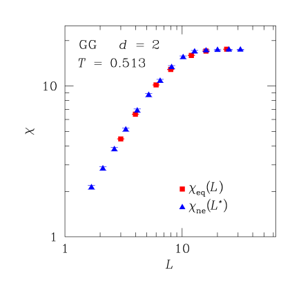
Figure 5: (Color online) Two-dimensional GG equilibrium (squares) and nonequilibrium (triangles) susceptibility data plotted as in Fig. 2, for $T=0.513$ with appropriate adjustment for optimum $A(T)$ and $z(T)$ for this temperature. In this figure $L^{*}(t_{\rm w})=1.346t_{\rm w}^{1/3.08}$.

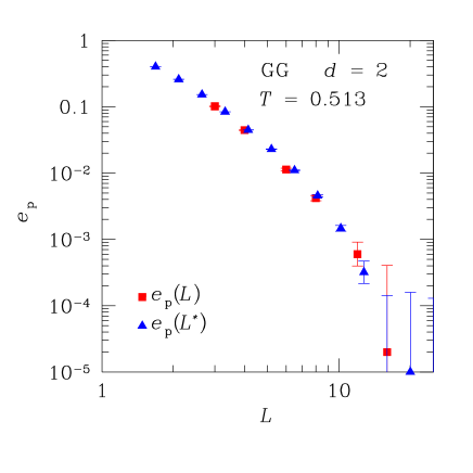
Figure 6: (Color online) Two-dimensional GG equilibrium (squares) and nonequilibrium (triangles) energy data are plotted as in Fig. 3, for $T=0.513$ with the same parameters $A(T)$ and $z(T)$ used in Fig. 5. In this figure $e_{\rm p}=e+1.263$.

The size-dependent equilibrium energy data $e_{\rm p}(L,T)=[e_{\rm eq}(L,T)-e(\infty,T)]$ and the time-dependent nonequilibrium energy data $e_{\rm p}(t,T)=[e_{\rm ne}(t_{\rm w},T)-e(\infty,T)]$ translated to $e_{\rm p}(L^{*},T)$ can also be plotted together assuming exactly the same scaling as for the susceptibility data as discussed above. To the present accuracy, for these temperatures the $z(T)$ values obtained from the energy data are indistinguishable from the values estimated from the susceptibility scaling [although the effective prefactors $A(T)$ are slightly different]. The errors in each $z(T)$ data point are subjective estimates obtained by varying the parameters around the optimal values.

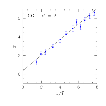
Figure 7: (Color online) Effective dynamical exponent $z(T)$ as a function of $1/T$ for the two-dimensional GG. The dashed line corresponds to a fit of the form $z(T)=2.18(9)+0.41(2)/T$ and is meant as a guide to the eye.

The estimates for $z(T)$ against $1/T$ are shown in Fig. 7. The data can be parametrized using

$$z(T)=2.18(9)+0.41(2)/T\;,$$ (15)

with $\chi^{2}\simeq 0.60$ for the fit. This implies a diverging dynamical exponent $z(T)$ as $T$ approaches zero and $z(T)$ tending to near $2$ at infinite temperature. Note that $z=2$ for a random walk.

We conclude from this section that for the GG in dimension 2 which orders at zero temperature, a time-dependent length scale $L^{*}(t_{\rm w},T)$ can be measured over a wide range of temperatures in the paramagnetic state. This length scale obeys the effective dynamical critical exponent scaling relationship, Eq. (5). The sets of values of $z(T)$ determined from the nonequilibrium spin-glass susceptibility $\chi_{\rm ne}(t_{\rm w},T)$ and the nonequilibrium energy per spin $e_{\rm ne}(t_{\rm w},T)$ are the same to within the present precision.

III.2 Three dimensions

The GG in dimension 3 has an ordering temperature $T_{\rm c}=0.46(1)$.Olson and Young (2000); Katzgraber and Campbell (2004) The analysis protocol used is essentially the same as in dimension 2 (Sec. III.1); parameters of the simulation are listed in the Appendix, Table 3 for equilibrium and Table 8 for nonequilibrium measurements, respectively. Below $T_{\rm c}$ and in the $L$ and $t_{\rm w}$ ranges that we have studied, the equilibrium susceptibility increases as $\chi_{\rm eq}(L,T)\propto L^{x(T)}$ and the nonequilibrium susceptibility as $\chi_{\rm ne}(t_{\rm w},T)\propto t_{\rm w}^{y(T)}$ with $T$-dependent $x(T)$ and $y(T)$. This algebraic behavior facilitates the analysis because the log-log plots of $\chi$ are all straight lines.

As in the two-dimensional case, at each temperature an effective dynamical exponent $z(T)$ and prefactor $A(T)$ can be defined from the scaling of the equilibrium and nonequilibrium susceptibility data using Eq. (5). As in two dimensions the energy data can be scaled satisfactorily using the same $z(T)$ obtained at each $T$ from the analysis of the susceptibility data. Below $T_{\rm c}$ the prefactors $A(T)$ are slightly different for both the energy, as well as the scaling of the susceptibility (not shown).

In three dimensions $z(T)$ also increases $\sim 1/T$ and has an intercept $z(\infty)\approx 2$—i.e.,

$$z(T)=1.95(8)+1.17(4)/T\;,$$ (16)

with $\chi^{2}\simeq 1.06$ for the fit.

The present estimate for $z_{\rm c}$ at $T_{\rm c}=0.46(1)$ is $z_{\rm c}=4.5(1)$, in agreement with previous estimates.Katzgraber and Campbell (2004)

It is important to note that $z(T)$ traverses $T_{\rm c}$ smoothly with no apparent anomaly; see Fig. 8. This implies that in terms of the evolution of length scales with time, the dynamics above and below the ordering temperature follow the same pattern although in the final equilibrium configuration all the spins are ordered below $T_{\rm c}$ and while they are only correlated over a finite length scale above $T_{\rm c}$. In this system the critical behavior is not exceptional as far as the length scale dynamics is concerned.

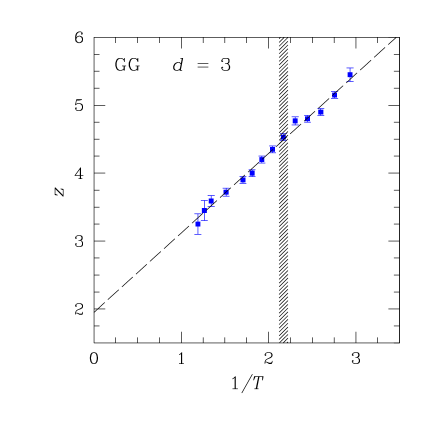
Figure 8: (Color online) Effective dynamical exponent $z(T)$ as a function of $1/T$ for the three-dimensional GG. The dashed line corresponds to a fit of the form $z(T)=1.95(8)+1.17(4)/T$. The shaded region denotes $T_{\rm c}=0.46(1)$. In this and the following figures, the width of the shaded area represents the error bar on the estimate of the critical temperature.

III.3 Four dimensions

The GG in four dimensions has an ordering transition at $T\approx 0.89(1)$.Katzgraber and Campbell (2004) We perform a similar analysis as done in the two- and three-dimensional case. Parameters of the simulation are listed in the Appendix, Tables 4 and 8. A very similar pattern of behavior is observed as in the GG with lower space dimensions, with $z(T)$ increasing linearly with inverse temperature—i.e.,

$$z(T)=1.75(13)+2.4(1)/T\;.$$ (17)

Here $\chi^{2}\simeq 0.3$ for the fit.

As in dimension 3 there is no sign of any change of behavior in the region of $T_{\rm c}$; see Fig. 9. At $T_{\rm c}\approx 0.89$ we obtain $z_{\rm c}=4.5(1)$, in agreement with Ref. Katzgraber and Campbell, 2004.

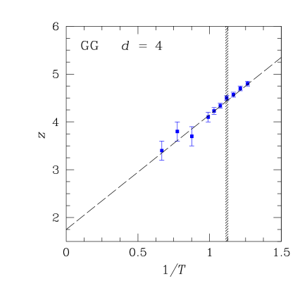
Figure 9: (Color online) Effective dynamical exponent $z(T)$ as a function of $1/T$ for the four-dimensional GG. The dashed line corresponds to a fit of the form $z(T)=1.75(13)+2.4(1)/T$. The shaded region denotes $T_{\rm c}=0.89(1)$.

IV Ising Spin Glass

The Hamiltonian of the Edwards-Anderson Ising spin glassEdwards and Anderson (1975) is given by

$${\cal H}=-\sum_{\langle i,j\rangle}J_{ij}S_{i}S_{j},$$ (18)

where the sum is over nearest-neighbor pairs of sites on a hypercubic lattice in $d$ dimensions, the $S_{i}$ are Ising spins taking values $\pm 1$, and the $J_{ij}$ are Gaussian distributed with zero mean and standard deviation unity. Simulations are done using periodic boundary conditions. Parameters of the simulation are listed in the Appendix.

IV.1 Two dimensions

As in the case of the two-dimensional GG, the EA ISG with Gaussian interactions in dimension 2 orders only at zero temperature;McMillan (1984); Bray and Moore (1984); Rieger et al. (1996); Palassini and Young (1999); Hartmann and Young (2001); Hartmann et al. (2002) thus, all the data concern the paramagnetic regime. Details of the simulations are summarized in the Appendix, Tables 5 and 9. The data show that an analysis according to Eq. (5) provides an excellent parametrization of the growth of correlations. The results are in good agreement with direct measurements of the correlation functions.Kisker et al. (1996); Rieger et al. (2004)

The energy per spin data, $e(t_{\rm w},T)$, can be parametrized consistently in terms of the same effective set of dynamical exponents $z(T)$ as used for the analysis of the $\chi(T)$ data.

The temperature dependence of $z(T)$ is much stronger than for the GG systems, and $z(T)$ deviates somewhat from a linear variation with inverse temperature; cf. Fig. 10. For $1/T\leq 5$, the $z(T)$ data can be approximately parametrized by $z(T)\simeq 3.9/T$. (It is possible that the curve could bend at low $1/T$ to a nonzero intercept.) The present analysis is consistent with those of Refs. Kisker et al., 1996 and Rieger et al., 2004, who obtain $z(T)\simeq 4.3/T$ using a different numerical technique. In Fig. 10 the dashed line is a quadratic fit in $x=1/T$ and should serve as a guide to the eye.

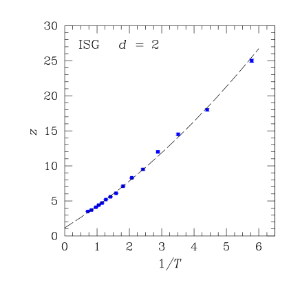
Figure 10: (Color online) The effective dynamical exponent $z(T)$ as a function of $1/T$ for the two-dimensional ISG. The line is a guide to the eye.

IV.2 Three dimensions

There is general consensus that the freezing temperature of the three-dimensional EA ISG with Gaussian interactions is $T_{\rm c}=0.94(2)$ (Refs. Marinari et al., 1998; Campbell et al., 2000; Ballesteros et al., 2000; Mari and Campbell, 2001) and that the dynamical critical exponent is $z_{\rm c}\simeq 6.45(10)$. The equilibrium SG susceptibility $\chi_{\rm eq}(L,T)$ and energy per spin, $e_{\rm eq}(L,T)$, are measured at temperatures between $T=0.1$ and $T=3.0$ for several intermediate sample sizes, see Table 6. Nonequilibrium measurements are made for $L_{\rm b}=24$; see Table 9. For temperatures up to $T_{\rm c}$ and for the range of sizes used, to a good approximation (as in the GG below $T_{\rm c}$)

$$\chi_{\rm eq}(L,T)=C(T)L^{x(T)}\;,$$ (19)

with $C(T)$ a temperature-dependent prefactor and $x(T)$ an effective exponent which becomes equal to the true static critical exponent $2-\eta$ at $T_{\rm c}$. $x(T)$ can never exceed $d$; for this system it reaches values very close to $3$ as $T$ tends to zero. $C(T)$ remains very close to $1$ for the whole temperature range. We can note that by definition $\chi_{\rm eq}(L=1)=1$ for all $T$. In the low-temperature range, for the equilibrium susceptibility $\chi_{\rm eq}(L,T)$ we make the assumption that $\log[\chi_{\rm eq}(L,T)]$ extrapolates linearly with $\log(L)$ to zero at $L=1$. ($L=2$ measurements have not been used, as at this particular size there are intrinsic “wrap-around” problems associated with the definition of the interactions.)

The effective dynamical critical exponent scaling parametrization analysis using Eq. (5) is satisfactory over the whole temperature range covered. Below $T_{\rm c}$, the present $z(T)$ values, Fig. 11, are consistent with those of Refs. Parisi et al., 1996 and Kisker et al., 1996 but more accurate. The prefactors $A(T)$ vary only slightly with $T$, and $A(T)\simeq 2B(T)$ where $B(T)$ are the prefactors for the coherence length $\ell(t_{\rm w},T)$ estimated by Refs. Parisi et al., 1996 and Kisker et al., 1996. This agreement confirms the conjecture made above that as a general rule the correlation length $\ell(t_{\rm w})$ can be taken as equal to $L^{*}(t_{\rm w})/2$ to a good approximation. For temperatures above $T_{\rm c}$, a scaling of the effective exponent form remains very satisfactory; see Fig. 11.

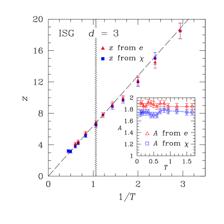
Figure 11: (Color online) The effective dynamical exponent $z(T)$ as a function of $1/T$ for the three-dimensional ISG. The line corresponds to a fit of the form $z(T)=6.40(15)/T$. The squares correspond to data for $z(T)$ as estimated from the energy, whereas the triangles represent data for $z(T)$ calculated using the spin-glass susceptibility. The inset shows the prefactor $A$ of the scaling relation in Eq. (5) as estimated for the energy and susceptibility. The data show little temperature dependence.

As found by Refs. Parisi et al., 1996 and Kisker et al., 1996, $z(T)$ varies approximately linearly with $1/T$. The present data (which are more accurate than those of the previous work), including points in the paramagnetic region up to about $2.5T_{\rm c}$, are consistent with $z(T)\simeq 6.40(15)/T$ ($\chi^{2}\simeq 0.85$). The points for $z(T)$ vary smoothly and continuously through $T_{\rm c}$, as in the three- and four-dimensional GG.

Again, one can carry out a scaling plot for the nonequilibrium energy $e_{\rm ne}(t_{\rm w},T)$ in the same way as for the susceptibility. The effective $z(T)$ values estimated from the energy scaling are consistent with the values from the susceptibility scaling, but the prefactors $A(T)$ become slightly different in the lower temperature range. This confirms that one single anneal-time-dependent length growth law controls both susceptibility and energy during the anneal, which seems a more satisfactory form of analysis than, for instance, that given in Sec. VI A of Ref. Yoshino et al., 2002.

It would be of interest to carry out further measurements so as to obtain significantly more information at low and moderate temperatures, but this would require nonequilibrium simulations extending to much longer annealing times.

IV.3 Four dimensions

For the EA ISG with Gaussian couplings in four dimensions it is known that $T_{\rm c}=1.78(2)$,Parisi et al. (1996); Bernardi and Campbell (1997); Campbell et al. (2000) with a dynamical critical exponent $z_{\rm c}=4.9(2)$.Bernardi and Campbell (1997); Campbell et al. (2000) The present data are analyzed in just the same way as for the three-dimensional ISG. There is excellent agreement between estimates for $z(T)$ between susceptibility and energy data.

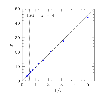
Figure 12: (Color online) The effective dynamical exponent $z(T)$ as a function of $1/T$ for the four-dimensional ISG. The line corresponds to a fit of the form $z(T)=9.15(20)/T$.

In four dimensions $z(T)$ varies approximately linearly with inverse temperature—i.e., $z(t)\simeq 9.15(20)/T$ with $\chi^{2}\simeq 2.8$; see Fig. 12. The estimate for $z$ at $T_{\rm c}$ is $z_{\rm c}=5.1(2)$, in agreement with previous work.Bernardi and Campbell (1997) Once more, $z(T)$ evolves smoothly as $T$ passes through $T_{\rm c}$.

V Summary

The observed behavior of the dynamical exponent $z(T)$ for the six systems studied is summarized in Table 1. It can be seen that for the GG systems the data in each dimension can be parametrized in the form $z(T)\simeq a+b/T$ with the constants $a\approx 2$ and $b$ increasing with dimension $d$. For the EA ISG systems, $z(T)\simeq b/T$—i.e., $a=0$, with $b$ values again increasing strongly with space dimension $d$; in each dimension the value of $b$ is higher than that of the GG by a factor of 5–10. For each of the ISG’s the data could be compatible with a nonzero infinite-temperature intercept if there is some curvature in $z(1/T)$ at temperatures higher than those we have studied. In two dimensions the data potentially suggest such a behavior.

Table 1: Temperature dependence of the dynamical exponent $z(T)=a+b/T$ for the different models studied at different space dimensions $d$. GG refers to the gauge glass, ISG to the Ising spin glass with Gaussian interactions. For the Ising spin glass in two dimensions the quoted value of $b$ corresponds to a linear fit which is a poor approximation to the behavior seen in this system (marked with an asterisk).

System	$d$	$a$	$b$
GG	$2$	$2.18(9)$	$0.41(2)$
GG	$3$	$1.95(8)$	$1.17(4)$
GG	$4$	$1.75(13)$	$2.4(1)$
ISG∗	$2$	$0$	$3.9(1)$
ISG	$3$	$0$	$6.40(15)$
ISG	$4$	$0$	$9.15(20)$

VI Droplet dynamics approach

We have obtained very satisfactory scaling of the Ising spin glass and gauge glass dynamics using the effective exponent parametrization, Eq. (5). We now discuss an alternative analysis based on the dynamical droplet approach, which distinguishes critical behavior near $T_{\rm c}$ from activated behavior with a barrier exponent $\psi$ further below $T_{\rm c}$.Bouchaud et al. (2001) Berthier and BouchaudBerthier and Bouchaud (2002, 2003) (BB) carried out four-spin correlation function measurements on the three-dimensional EA ISG similar to those of Refs. Parisi et al., 1996 and Kisker et al., 1996, but analyzed their data on the basis of the droplet dynamics formula.Bouchaud et al. (2001)

A similar analysis of Heisenberg spin-glass dynamics (see Fig. 11 of Ref. Berthier and Young, 2004) shows qualitatively different behavior from that of the systems reported here. We have no data on Heisenberg systems although the present technique could potentially be applied there as well.

The BB droplet dynamics leads to a growth law with time corresponding to a coherence length $\ell(t)$

$$t_{\rm w}[\ell(t,T)]\simeq\tau^{*}[\ell(t,T)]^{z_{\rm c}}\exp[\Upsilon(T)\ell(t,T)^{\psi}/T]\;,$$ (20)

where $z_{\rm c}$ is the dynamical critical exponent, $\psi$ is the barrier exponent, $\Upsilon(T)=\Upsilon_{0}(1-T/T_{\rm c})^{\nu\psi}$, and $\tau^{*}$ is a prefactor. BB scale the data using $z_{\rm c}=7$, $\nu=1.65$, $\psi=1$, and $\Upsilon_{0}=5.5$ and assume $\tau^{*}\sim 2$ but to find good overall fits they needed to choose temperature-dependent values for $\tau^{*}$.

Yoshino et al.Yoshino et al. (2002) made a closely related analysis of measurements on the four-dimensional $\pm J$ ISG. They introduce a “crossover length”

$$L_{0}(T)=T^{1/\psi}(1-T/T_{\rm c})^{-\nu}$$ (21)

and a “crossover time”

$$\tau_{0}(T)=[L_{0}(T)]^{z_{\rm c}}$$ (22)

together with a general scaling law for the coherence length,

$$\ell(t_{\rm w})/L_{0}(T)=f_{\ell}[t_{\rm w}/\tau_{0}(T)]\;,$$ (23)

which relates the coherence length $\ell(t_{\rm w})$ to the elapsed time $t_{\rm w}$. Here $f_{\ell}$ represents an unknown scaling function. The scaling curve depends on the critical parameters ($T_{\rm c}$, $z_{\rm c}$, and $\nu$) which can be taken as known from measurements at $T_{\rm c}$, and on the barrier exponent $\psi$. It can be readily shown that the BB equation, Eq. (20), is an inversion of the scaling equation of Yoshino et al., Eq. (23), with an explicit functional form which can be written as

$$t_{\rm w}/\tau_{0}(T)=\tau^{*}[\ell(t_{\rm w})/L_{0}(T)]^{z_{\rm c}}\exp\{\Upsilon_{0}[\ell(t_{\rm w})/L_{0}(T)]^{\psi}\}\;.$$ (24)

We now analyze the present data for the EA ISG in three dimensions in terms of the BB/Yoshino droplet dynamics approach.com (c) In Fig. 13 we plot the present data in three dimensions for $L^{*}(t_{\rm w},T)$ as a function of $t_{\rm w}$ at different $T$ in the scaling form proposed by Yoshino et al.;Yoshino et al. (2002) i.e., we plot $L^{*}(t_{\rm w},T)/2L_{0}(T)$ against $t_{\rm w}/\tau_{0}(T)$ with $L_{0}(T)=T^{1/\psi}(1-T/T_{\rm c})^{-\nu}$ and $\tau_{0}=[L_{0}(T)]^{z_{\rm c}}$ [the factor $1/2$ corresponds to the translation from $L^{*}(t_{\rm w},T)$ to $\ell(t_{\rm w},T)$] (see inset of Fig. 11). For this scaling we adopt for the three-dimensional EA system the parameters proposed by BB: $z_{\rm c}=7$, $\nu=1.65$, and $\psi=1$. According to Yoshino et al., the entire data set scaled this way should lie on a single (but unspecified) scaling curve. The extra BB scaling parameters define one specific scaling curve within the same plot. On the “Yoshino plot” we therefore draw the full BB scaling plot, Eq. (24), using the two remaining fit parameters from the BB parameter set: $\Upsilon_{0}=5.5$ and $\tau^{*}=2$.

In the temperature region from $T_{\rm c}$ down to about $T_{\rm c}/2$ the overall Yoshino scaling and the agreement between the present data and the BB scaling curve is acceptable. This is the same temperature range as covered by the BB simulations. However, in the temperature range below $T_{\rm c}/2$ where the activated droplet dynamics should be valid because little is affected by critical dynamics, the scaling breaks down. The curves for different $T$ are not superimposed, and the deviations from the BB curve correspond to many orders of magnitude along the time axis.

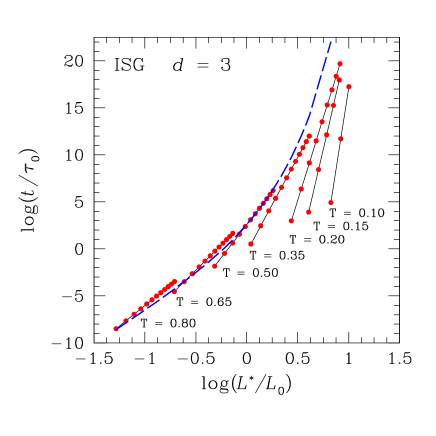
Figure 13: (Color online) Three-dimensional ISG data plotted following to the parametrization of Yoshino et al. (Ref. Yoshino et al., 2002). According to this droplet dynamics approach all the data presented in this way should lie on a single scaling curve. The long-dashed line is the particular scaling curve calculated using the specific parameters proposed by Berthier and Bouchaud in Ref. Berthier and Bouchaud, 2002 for this system. For the definitions of the parameters $L_{0}$ and $\tau_{0}$ see the text, Eqs. (21) and (22), respectively.

An analysis of the EA ISG data in four dimensions leads to the same conclusion. The measurements of Yoshino et al.Yoshino et al. (2002) were made on the $\pm J$ model while the present measurements correspond to the model with Gaussian disorder, but if we adopt the critical parameters $T_{\rm c}=1.8$, $z_{\rm c}=4.5$, and $\nu=0.93$, together with $\psi=4.5$ from Yoshino et al.,Yoshino et al. (2002) we obtain an overall scaling plot for the present EA ISG results in four dimensions. Once again the agreement between the scaling prediction (a unique scaling curve) and the data set is acceptable for temperatures $T_{\rm c}/2\leq T\leq T_{\rm c}$, but it breaks down at lower temperatures (not shown).

Thus for these two canonical ISG systems the standard droplet dynamics scaling below $T_{\rm c}$ does not give a satisfactory global account of the data; by suitably adjusting the various fit parameters the droplet scaling relation, Eq. (23), can be made to conform reasonably well to the data over limited ranges of temperature and annealing time, but at low temperatures this form of scaling predicts a time scale $t/\tau_{0}$ which diverges much more rapidly with increasing length scale $L^{*}/L_{0}$ than is observed.

If we attempt to determine $\psi$ for the three-dimensional GG from scaling our data using this droplet expression, we find only poor scaling whatever $\psi$ values are assumed for a very wide range of values.

Kisker et al.,Kisker et al. (1996) as well as fitting very successfully their EA ISG data in two and three dimensions to Eq. (5), also compared their data to a different phenomenological droplet-dynamics-inspired formula:

$$\ell(t_{\rm w})-\ell_{0}=\lambda(T)[\ln(t_{\rm w})]^{1/\psi}$$ (25)

and found that this relation was capable of giving a satisfactory fit to their low-temperature data. However, as they point out in Ref. Kisker et al., 1996, this formulation has a number of defects; in particular, one would not expect the droplet formula to be applicable in the paramagnetic region. We can also examine the mathematical basis of the equation. Suppose that the true time dependence is $\ell(t_{\rm w})=At_{\rm w}^{1/z}$—i.e., $\ln[\ell(t_{\rm w})]=\ln(A)+(1/z)\ln(t_{\rm w})$—with $z$ large. The parametrization, Eq. (25), can be recast as $\ell(t_{\rm w})=\ell_{0}\cdot(1+x)$ or $\ln[\ell(t_{\rm w})]=\ln(\ell_{0})+\ln(1+x)$, with $x=[B\ln(t_{\rm w})]^{1/\psi}$, where $B=(\lambda(T)/\ell_{0})^{\psi}$ is small. Because $\ln(1+x)=x-x^{2}/2+...$, we have $\ln[\ell(t_{\rm w})]=\ln(\ell_{0})+[B\ln(t_{\rm w})]^{1/\psi}-[B\ln(t_{\rm w})]^{2/\psi}/2+\cdots$. If $1/\psi>1$, on a $\log[\ell(t_{\rm w})]$ against $\log(t_{\rm w})$ plot there will be an upbending from the second term compensated by a growing negative third term. Trial and error shows that if $\psi\simeq 2/3$, this parametrization produces to quite good accuracy a linear dependence of $\log[\ell(t_{\rm w})]$ on $\log(t_{\rm w})$ over a wide range of $t_{\rm w}$, typically from $t_{\rm w}=10$ to $t_{\rm w}=10^{8}$, successfully mimicking $\ln[\ell(t_{\rm w})]=\ln(A)+(1/z)\ln(t_{\rm w})$. Thus a fit to the parametrization in Eq. (25) can be obtained with a pseudo “barrier exponent” $\psi$ even when the true behavior is better described by $\ell(t_{\rm w})=At_{\rm w}^{1/z}$, so this fit is a mathematical artifact. The value of $\psi$ obtained from such a fit can be expected to be $\simeq 2/3$ regardless of the system studied, which explains why the apparent $\psi$ estimated in Ref. Kisker et al., 1996 both for the three-dimensional ISG well below $T_{\rm c}$ and for the paramagnetic two-dimensional ISG at low temperatures are close to this value.

We conclude from this section that the standard droplet scaling approach does not give a satisfactory overall account of the numerical Ising spin-glass dynamical data in dimensions 3 and 4.

VII Conclusion

We have studied the dynamical behavior of ISG’s and GG’s in dimensions 2, 3, and 4 as functions of anneal time $t_{\rm w}$ after a quench to a temperature $T$. We define a time-dependent correlation length scale $L^{*}(t_{\rm w},T)$ by relating the time-dependent nonequilibrium susceptibility $\chi_{\rm ne}(t_{\rm w},T)$ to the size-dependent equilibrium susceptibility $\chi_{\rm eq}(L,T)$ and the time-dependent energy $e_{\rm ne}(t_{\rm w},T)$ data to the equilibrium energy $e_{\rm eq}(L,T)$ data. In each system and at all temperatures (below and above the freezing temperature $T_{\rm c}$, as well as at $T_{\rm c}$) a growth law for the length scale $L^{*}(t_{\rm w},T)=A(T)t_{\rm w}^{1/z(T)}$ gives a good parametrization of the data, with an effective temperature-dependent dynamical exponent $z(T)$ and a prefactor $A(T)$ which is only weakly temperature dependent. In each case, independent estimates of $z(T)$ from the susceptibility and from the energy measurements are the same within the precision of the measurements; the prefactors $A(T)$ corresponding to the susceptibility and to the energy can be marginally different. $z(T)$ diverges approximately as $1/T$ at low temperatures in all the systems, and at high temperatures it appears to tend to a limiting value consistent with $z(\infty)\sim 2$ for the GG systems and to a value which extrapolation suggests is close to zero for the ISG systems. The evolution of $z(T)$ as the temperature passes through the freezing temperature $T_{\rm c}$ is smooth for all four systems having a nonzero $T_{\rm c}$. In the Ising spin glasses the dynamic droplet critical scaling approachBerthier and Bouchaud (2002); Yoshino et al. (2002) is incompatible with the present measurements for the region below $T_{\rm c}/2$. The droplet picture gives no predictions whatsoever concerning time-length relationships in the paramagnetic region above $T_{\rm c}$. The data show that the standard droplet dynamics assumptionsFisher and Huse (1986, 1988, 1988); Bouchaud et al. (2001) of an effective barrier height increasing as a power of $\ell$ and disappearing at $T_{\rm c}$ are inappropriate for the systems studied.

Many recent experimental measurements of dynamics in spin glassesDupuis et al. (2001); Bouchaud et al. (2001); Jönsson et al. (2002b); Bert et al. (2004) have been interpreted using the droplet dynamics parametrization. It is nontrivial to transpose conclusions obtained from numerical data to the experimental regime; the effective time scales for experiments are vastly greater than for the numerical results, and length scales are slightly larger. It must also be kept in mind that there appears to be no way in which to measure spin-glass coherence lengths directly from experiment. As the present results invalidate the standard droplet dynamics in Ising spin glasses at least on time scales attainable numerically, the question should be raised as to what physical significance, if any, can be ascribed to parameters such as the barrier exponent $\psi$ which are obtained from scaling analyses of experimental data based on standard droplet dynamics. As has been pointed out in Ref. Jönsson et al., 2004, for one canonical ISG system the range of published estimates of $\psi$ from different experiments extends from $0.03$ to $1.9$,Mattsson et al. (1995); Dupuis et al. (2001); Bouchaud et al. (2001); Jönsson et al. (2002b); Bert et al. (2004) which also suggests that the standard droplet dynamics parametrization is inappropriate. Recently, a rigorous bound for the barrier exponent inferred from two-dimensional calculationsAmoruso et al. (2005) has been given with $0.25<\psi<0.54$. Still, it would seem well worth attempting to review the experimental data to see if they can be reinterpreted in terms of an effective exponent length scale growth scenario compatible with the present numerical results.

The effective dynamical critical exponent scaling scenario with $z(T)\propto 1/T$ which provides a satisfactory parametrization for the ISG systems is very similar to that observed by Paul et al.Paul et al. (2004, 2005) for random-bond Ising ferromagnets (RBIM’s) and diluted ferromagnets in dimension 2. The physical mechanism for the time dependence of the correlation length in these ferromagnetic models is domain coarsening, and the data are interpreted in terms of effective barriers to domain growth which increase logarithmically with size.Rieger (1993) It would seem very plausible to ascribe the correlation length growth in spin glasses to an analogous mechanism. Equation (9) of Paul et al.Paul et al. (2004, 2005) can be written as $z(T)=2+c/T$, $c$ a constant, in our terminology, which is precisely what we have observed empirically for the GG systems. However, it should be noted that at the ordering temperature $T_{\rm c}$ for the RBIM the effective dynamical exponent tends to the pure system value $z\sim 2$.Paul et al. (2004) In the ISG’s and GG’s the dynamical critical exponent $z_{\rm c}$ is always much higher than $2$ and $z(T)$ continues to decrease regularly as the temperature is raised through the paramagnetic regime. This is true both above the ordering temperature when $T_{\rm c}$ is nonzero or at all temperatures when $T_{\rm c}=0$ which is the case in dimension 2.

The standard approach to the dynamics of the growth of the coherence length $\ell(t_{\rm w})$ with anneal time after quench $t_{\rm w}$ is to assume that there are three principal relaxation regimes: paramagnetic at temperatures well above $T_{\rm c}$, critical in the region around $T_{\rm c}$, and activated at temperatures well below $T_{\rm c}$, each regime having a qualitatively different relaxation behavior. The present data show that for Ising spin glasses and for the gauge glass, a dynamical relationship of the standard critical form, $\ell(t_{\rm w})=A(T)t_{\rm w}^{1/z(T)}$ with a temperature-dependent dynamical exponent $z(T)$, gives a good account of the nonequilibrium dynamics at each temperature and not only at $T_{\rm c}$. The data indicate that $z(T)$ varies smoothly as a function of temperature when passing through $T_{\rm c}$.

*

Appendix A Numerical Details

Equilibrium measurements are carried out with samples fully thermalized using the exchange Monte Carlo (parallel tempering) technique.Hukushima and Nemoto (1996); Marinari et al. (1996) To ensure that the system is equilibrated, we perform a logarithmic data binning of all observables (energy and spin-glass susceptibility) and require that the last three bins logarithmically spaced agree within error bars and be independent of the number of Monte Carlo sweeps (MCS) $N_{\mathrm{sweep}}$. In the case of the Ising spin glass we use the equilibration test for short-range spin glasses first introduced in Ref. Katzgraber et al., 2001. Details about the equilibrium simulations for the gauge glass are summarized in Tables 2, 3, and 4, for $d=2$, $3$, and $4$, respectively. Details about the equilibrium simulations for the Ising spin glass are presented in Tables 5, 6, and 7, for $d=2$, $3$, and $4$, respectively. For all runs we ensure that the parallel tempering Monte Carlo moves have acceptance probabilities of at least 30%.

Table 2: Parameters of the equilibrium simulations for the two-dimensional gauge glass. $N_{\mathrm{samp}}$ is the number of samples, $N_{\mathrm{sweep}}$ is the total number of Monte Carlo sweeps for each of the $2N_{T}$ copies (two replicas per temperature) for a single sample, and $N_{T}$ is the number of temperatures used in the parallel tempering method. The lowest temperature used is $0.13$, the highest $1.058$. For $L=24$ the lowest temperature studied is $0.20$.

$L$	$N_{\mathrm{samp}}$	$N_{\mathrm{sweep}}$	$N_{T}$
3	$10\;000$	$8.0\times 10^{4}$	30
4	$10\;400$	$8.0\times 10^{4}$	30
6	$10\;150$	$8.0\times 10^{4}$	30
8	$8\;495$	$2.0\times 10^{5}$	30
12	$6\;890$	$8.0\times 10^{5}$	30
16	$2\;500$	$2.0\times 10^{6}$	30
24	$2\;166$	$2.0\times 10^{6}$	24

Table 3: Parameters of the equilibrium simulations for the three-dimensional gauge glass. The lowest temperature simulated is $0.05$, the highest $0.947$. The different quantities are explained in the caption of Table 2.

$L$	$N_{\mathrm{samp}}$	$N_{\mathrm{sweep}}$	$N_{T}$
3	$10\;000$	$6.0\times 10^{3}$	53
4	$10\;000$	$2.0\times 10^{4}$	53
5	$10\;000$	$6.0\times 10^{4}$	53
6	$5000$	$2.0\times 10^{5}$	53
8	$2000$	$1.2\times 10^{6}$	53

Table 4: Parameters of the equilibrium simulations for the gauge glass in four dimensions. The lowest temperature used is $0.70$, the highest $1.345$. The different quantities are explained in the caption of Table 2.

$L$	$N_{\mathrm{samp}}$	$N_{\mathrm{sweep}}$	$N_{T}$
3	$5000$	$2.0\times 10^{4}$	17
4	$5000$	$8.0\times 10^{4}$	17
5	$5000$	$4.0\times 10^{5}$	17

Table 5: Parameters of the equilibrium simulations for the Ising spin glass in two dimensions. The different quantities are explained in the caption of Table 2. For $L=128$ the minimum temperature used is $0.20$. For all other system sizes the minimum temperature is $0.05$. The maximum temperature used is $1.391$. Note that for $L\leq 16$ standard parallel tempering Monte Carlo is used, whereas for $L\geq 32$ the cluster method by Houdayer (Ref. Houdayer, 2001) is applied.

$L$	$N_{\mathrm{samp}}$	$N_{\mathrm{sweep}}$	$N_{T}$
3	$10\;000$	$2.0\times 10^{5}$	20
4	$10\;000$	$2.0\times 10^{5}$	20
6	$10\;000$	$2.0\times 10^{5}$	20
8	$10\;000$	$2.0\times 10^{5}$	20
10	$10\;000$	$1.0\times 10^{6}$	20
12	$10\;000$	$1.0\times 10^{6}$	20
16	$10\;000$	$1.0\times 10^{6}$	20
24	$10\;000$	$1.0\times 10^{5}$	20
32	$10\;000$	$1.0\times 10^{5}$	20
64	$1000$	$1.0\times 10^{6}$	40
128	$250$	$1.0\times 10^{6}$	63

Table 6: Parameters of the equilibrium simulations for the Ising spin glass in three dimensions. The lowest temperature used in the parallel tempering method is $0.10$, the highest $2.00$. Additional higher temperatures have been computed with simple Monte Carlo. The different quantities are explained in the caption of Table 2.

$L$	$N_{\mathrm{samp}}$	$N_{\mathrm{sweep}}$	$N_{T}$
3	$20\;000$	$5.0\times 10^{3}$	18
4	$30\;000$	$5.0\times 10^{3}$	18
5	$10\;000$	$5.0\times 10^{4}$	18
6	$10\;000$	$1.5\times 10^{5}$	18
8	$10\;000$	$5.0\times 10^{6}$	18

Table 7: Parameters of the equilibrium simulations for the Ising spin glass in four dimensions. The lowest temperature used in the parallel tempering method is $0.20$, the highest $2.80$. Additional higher temperatures have been computed with simple Monte Carlo. The different quantities are explained in the caption of Table 2.

$L$	$N_{\mathrm{samp}}$	$N_{\mathrm{sweep}}$	$N_{T}$
3	$60\;000$	$6.0\times 10^{3}$	12
4	$30\;000$	$6.0\times 10^{4}$	12
5	$12\;190$	$3.0\times 10^{5}$	23

Parameters used in the nonequilibrium simulations are summarized in Tables 8 and 9 for the GG, as well as the ISG, respectively.

Table 8: Parameters of the off-equilibrium simulations as a function of space dimension $d$ for the GG. $L_{\rm b}$ is the size of the system used and $t_{\rm w}$ is the “waiting time.” $N_{\mathrm{samp}}$ is the number of samples used for the disorder average. The same temperature sets as in the equilibrium simulations have been used.

$d$	$L_{\rm b}$	$N_{\mathrm{samp}}$	$t_{\rm w}$
$2$	$64$	$1000$	$1.638\times 10^{4}$
$3$	$16$	$1000$	$8.192\times 10^{3}$
$4$	$10$	$1000$	$1.310\times 10^{5}$

Table 9: Parameters of the off-equilibrium simulations as a function of space dimension $d$ for the ISG. The different quantities are explained in the caption of Table 8. The same temperature sets as in the equilibrium simulations have been used.

$d$	$L_{\rm b}$	$N_{\mathrm{samp}}$	$t_{\rm w}$
$2$	$128$	$1000$	$32\;768$
$3$	$24$	$1000$	$32\;768$
$4$	$10$	$1000$	$32\;768$

By convention, values quoted at time $t$ correspond to an average taken between MCS’s $[t+1]$ to $[2t]$ following an anneal of $t$ MCS’s.

References

- Binder and Young (1986) K. Binder and A. P. Young, Spin glasses: Experimental facts, theoretical concepts and open questions, Rev. Mod. Phys. 58, 801 (1986).
- Young (1998) A. P. Young, ed., Spin Glasses and Random Fields (World Scientific, Singapore, 1998).
- Dupuis et al. (2001) V. Dupuis, E. Vincent, J.-P. Bouchaud, J. Hammann, A. Ito, and H. A. Katori, Aging, rejuvenation, and memory effects in Ising and Heisenberg spin glasses, Phys. Rev. B 64, 174204 (2001).
- Bouchaud et al. (2003) J.-P. Bouchaud, F. Krzakala, and O. C. Martin, Energy exponents and corrections to scaling in Ising spin glasses, Phys. Rev. B 68, 224404 (2003).
- Jönsson et al. (2002a) P. E. Jönsson, H. Yoshino, P. Nordblad, H. ArugaKatori, and A. Ito, Domain growth by isothermal aging in 3d Ising and Heisenberg spin glasses, Phys. Rev. Lett. 88, 257204 (2002a).
- Bert et al. (2004) F. Bert, V. Dupuis, E. Vincent, J. Hammann, and J.-P. Bouchaud, Spin Anisotropy and Slow Dynamics in Spin Glasses, Phys. Rev. Lett 92, 167203 (2004).
- Jimenez et al. (2004) S. Jimenez, V. Martin-Mayor, and S. Perez-Gaviro, Rejuvenation and memory in model spin glasses in 3 and 4 dimensions, (cond-mat/0406345) (2004).
- Berthier and Young (2005) L. Berthier and A. P. Young, Temperature Cycles in the Heisenberg Spin Glass (2005), (cond-mat/0503012).
- Huse (1989) D. A. Huse, Remanent magnetization decay at the spin-glass critical point: A new dynamic critical exponent for nonequilibrium autocorrelations, Phys. Rev. B 40, 304 (1989).
- Jannsen et al. (1989) H. K. Jannsen, B. Schaub, and B. Schmitman, Z. Phys. B 73, 539 (1989).
- com (a) Note that we use the convention by Berthier and Young (Ref. Berthier and Young, 2004) where represents a time after quench, whereas refers to a time difference.
- Zheng et al. (1999) B. Zheng, M. Schulz, and S. Trimper, Dynamic simulations of the Kosterlitz-Thouless phase transition, Phys. Rev. E 59, R1351 (1999).
- Blundell et al. (1992) R. E. Blundell, K. Humayun, and A. J. Bray, Dynamic exponent of the 3D Ising spin glass, J. Phys. A 25, L733 (1992).
- Mari and Campbell (2002) P. O. Mari and I. A. Campbell, The ordering temperature and critical exponents of the bimodal Ising spin glass in dimension three, Phys. Rev. B 65, 184409 (2002).
- Bernardi and Campbell (1997) L. W. Bernardi and I. A. Campbell, Critical exponents in Ising spin glasses, Phys. Rev. B 56, 5271 (1997).
- Katzgraber and Campbell (2004) H. G. Katzgraber and I. A. Campbell, Critical properties of the three- and four-dimensional gauge glass, Phys. Rev. B 69, 094413 (2004).
- Berthier and Bouchaud (2002) L. Berthier and J. P. Bouchaud, Geometrical aspects of aging and rejuvenation in the Ising spin glass: A numerical study, Phys. Rev. B 66, 054404 (2002).
- Parisi et al. (1996) G. Parisi, F. Ricci-Tersenghi, and J. J. Ruiz-Lorenzo, Equilibrium and off-equilibrium simulations of the 4d Gaussian spin glass, J. Phys. A 29, 7943 (1996).
- Kisker et al. (1996) J. Kisker, L. Santen, M. Schreckenberg, and H. Rieger, Off-equilibrium dynamics in finite-dimensional spin-glass models, Phys. Rev. B 53, 6418 (1996).
- Yoshino et al. (2002) H. Yoshino, K. Hukushima, and H. Takayama, Extended droplet theory for aging in short-range spin glasses and a numerical examination, Phys. Rev. B 66, 064431 (2002).
- Fisher and Huse (1988) D. S. Fisher and D. A. Huse, Nonequilibrium dynamics of spin glasses, Phys. Rev. B 38, 373 (1988).
- Fisher and Huse (1988) D. S. Fisher and D. A. Huse, Equilibrium behavior of the spin-glass ordered phase, Phys. Rev. B 38, 386 (1988).
- Mattsson et al. (1995) J. Mattsson, T. Jonsson, P. Nordblad, H. ArugaKatori, and A. Ito, No Phase Transition in a Magnetic Field in the Ising Spin Glass Fe0.5Mn0.5TiO3, Phys. Rev. Lett. 74, 4305 (1995).
- Bouchaud et al. (2001) J. P. Bouchaud, V. Dupuis, J. Hammann, and E. Vincent, Separation of time and length scales in spin glasses: Temperature as a microscope, Phys. Rev. B 65, 024439 (2001).
- Jönsson et al. (2002b) P. E. Jönsson, H. Yoshino, and P. Nordblad, Symmetrical Temperature-Chaos Effect with Positive and Negative Temperature Shifts in a Spin Glass, Phys. Rev. Lett. 89, 097201 (2002b).
- Rieger et al. (2004) H. Rieger, G. Scher, and R. Paul, Growing length scales during aging in 2d disordered systems, (cond-mat/0411234) (2004).
- Kosterlitz and Akino (1998) J. M. Kosterlitz and N. Akino, Numerical study of order in a gauge glass model, Phys. Rev. Lett. 81, 4672 (1998).
- Olson and Young (2000) T. Olson and A. P. Young, Finite temperature ordering in the three-dimensional gauge glass, Phys. Rev. B 61, 12467 (2000).
- Akino and Kosterlitz (2002) N. Akino and J. M. Kosterlitz, Domain wall renormalization group study of XY model with quenched random phase shifts, Phys. Rev. B 66, 054536 (2002).
- Simkin (1996) M. V. Simkin, Comment on “Voltage-Current Characteristics of the Two-Dimensional Gauge Glass Model” (1996), (cond-mat/9604178).
- Granato (1998) E. Granato, Current-voltage scaling of chiral and gauge-glass models of two-dimensional superconductors, Phys. Rev. B 58, 11161 (1998).
- Katzgraber (2003) H. G. Katzgraber, On the existence of a finite-temperature transition in the two-dimensional gauge glass, Phys. Rev. B 67, 180402(R) (2003).
- Katzgraber and Young (2001) H. G. Katzgraber and A. P. Young, Nature of the spin-glass state in the three-dimensional gauge glass, Phys. Rev. B 64, 104426 (2001).
- Fisher et al. (1991) M. P. A. Fisher, T. A. Tokuyasu, and A. P. Young, Vortex variable-range-hopping resistivity in superconducting films, Phys. Rev. Lett. 66, 2931 (1991).
- Gingras (1992) M. J. P. Gingras, Numerical study of vortex-glass order in random-superconductor and related spin-glass models, Phys. Rev. B 45, R7547 (1992).
- Reger and Young (1993) J. D. Reger and A. P. Young, Monte carlo study of a vortex glass model, J. Phys. A 26, 1067 (1993).
- Katzgraber and Young (2002) H. G. Katzgraber and A. P. Young, Numerical studies of the two- and three-dimensional gauge glass at low temperature, Phys. Rev. B 66, 224507 (2002).
- com (b) In order to save space only representative figures for the two-dimensional gauge glass are displayed.
- Edwards and Anderson (1975) S. F. Edwards and P. W. Anderson, Theory of spin glasses, J. Phys. F: Met. Phys. 5, 965 (1975).
- McMillan (1984) W. L. McMillan, Domain-wall renormalization-group study of the two-dimensional random Ising model, Phys. Rev. B 29, 4026 (1984).
- Bray and Moore (1984) A. J. Bray and M. A. Moore, Lower critical dimension of Ising spin glasses: a numerical study, J. Phys. C 17, L463 (1984).
- Rieger et al. (1996) H. Rieger, L. Santen, U. Blasum, M. Diehl, M. Jünger, and G. Rinaldi, The critical exponents of the two-dimensional Ising spin glass revisited: exact ground-state calculations and Monte Carlo simulations, J. Phys. A 29, 3939 (1996).
- Palassini and Young (1999) M. Palassini and A. P. Young, Evidence for a trivial ground state structure in the two-dimensional Ising spin glass, Phys. Rev. B 60, R9919 (1999).
- Hartmann and Young (2001) A. K. Hartmann and A. P. Young, Lower critical dimension of Ising spin glasses, Phys. Rev. B 64, 180404(R) (2001).
- Hartmann et al. (2002) A. K. Hartmann, A. J. Bray, A. C. Carter, M. A. Moore, and A. P. Young, The stiffness exponent of two-dimensional Ising spin glasses for non-periodic boundary conditions using aspect-ratio scaling, Phys. Rev. B 66, 224401 (2002).
- Marinari et al. (1998) E. Marinari, G. Parisi, and J. J. Ruiz-Lorenzo, On the phase structure of the 3d Edwards Anderson spin glass, Phys. Rev. B 58, 14852 (1998).
- Campbell et al. (2000) I. A. Campbell, D. Petit, P. O. Mari, and L. W. Bernardi, Critical exponents in Spin Glasses: numerics and experiments, J. Phys. Soc. Jap. Suppl. A 69, 186 (2000).
- Ballesteros et al. (2000) H. G. Ballesteros, A. Cruz, L. A. Fernandez, V. Martin-Mayor, J. Pech, J. J. Ruiz-Lorenzo, A. Tarancon, P. Tellez, C. L. Ullod, and C. Ungil, Critical behavior of the three-dimensional Ising spin glass, Phys. Rev. B 62, 14237 (2000).
- Mari and Campbell (2001) P. O. Mari and I. A. Campbell, Ising spin glasses: interaction distribution dependence of the critical exponents (2001), (cond-mat/0111174).
- Berthier and Bouchaud (2003) L. Berthier and J. P. Bouchaud, Comment on “Symmetrical Temperature-Chaos Effect with Positive and Negative Temperature Shifts in a Spin Glass”, Phys. Rev. Lett. 90, 059701 (2003).
- Berthier and Young (2004) L. Berthier and A. P. Young, Aging dynamics of the Heisenberg spin glass, Phys. Rev. B 69, 184423 (2004).
- com (c) A similar analysis in four dimensions (not shown) shows qualitatively similar results.
- Fisher and Huse (1986) D. S. Fisher and D. A. Huse, Ordered phase of short-range Ising spin-glasses, Phys. Rev. Lett. 56, 1601 (1986).
- Jönsson et al. (2004) P. E. Jönsson, H. Takayama, H. Aruga Katori, and A. Ito, Dynamical breakdown of the Ising spin-glass order under a magnetic field, (cond-mat/0411291) (2004).
- Amoruso et al. (2005) C. Amoruso, A. K. Hartmann, and M. A. Moore, Determining Energy Barriers by Iterated Optimization: The Two-Dimensional Ising Spin Glass (2005), (cond-mat/0502201).
- Paul et al. (2004) R. Paul, S. Puri, and H. Rieger, Domain growth in random magnets, Europhys. Lett. 68, 881 (2004).
- Paul et al. (2005) R. Paul, S. Puri, and H. Rieger, Domain Growth in Ising Systems with Quenched Disorder, (cond-mat/0502541) (2005).
- Rieger (1993) H. Rieger, Nonequilibrium dynamics and aging in the three-dimensional Ising spin-glass model, J. Phys. A 26, L615 (1993).
- Katzgraber et al. (2004) H. G. Katzgraber, L. W. Lee, and A. P. Young, Correlation Length of the Two-Dimensional Ising Spin Glass with Gaussian Interactions, Phys. Rev. B 70, 014417 (2004).
- Hukushima and Nemoto (1996) K. Hukushima and K. Nemoto, Exchange Monte Carlo method and application to spin glass simulations, J. Phys. Soc. Jpn. 65, 1604 (1996).
- Marinari et al. (1996) E. Marinari, G. Parisi, J. J. Ruiz-Lorenzo, and F. Ritort, Numerical evidence for spontaneously broken replica symmetry in 3d spin glasses, Phys. Rev. Lett. 76, 843 (1996).
- Katzgraber et al. (2001) H. G. Katzgraber, M. Palassini, and A. P. Young, Monte Carlo simulations of spin glasses at low temperatures, Phys. Rev. B 63, 184422 (2001).
- Houdayer (2001) J. Houdayer, A cluster Monte Carlo algorithm for 2-dimensional spin glasses, Eur. Phys. J. B. 22, 479 (2001).