THEORY OF SPIN-WAVE FREQUENCY GAPS IN 3D MAGNONIC CRYSTALS. APPLICATION TO MANGANITES.

Abstract

This study is an investigation of spin wave spectrum in macrostructures composed of two ferromagnetic materials and showing a 3D periodicity: spherical ferromagnetic grains disposed in the nodes of a 3D crystal lattice are embedded in a matrix with different ferromagnetic properties. Frequency ranges forbidden to spin wave propagation are found in the calculated magnonic spectra. Both the position and the width of the gaps are found to depend on the magnetic (exchange and magnetization) contrasts in the composite material, as well as on its structural parameters (filling fraction, crystal lattice type). Having applied our theory to interpretation of the existence of a spin wave gap in doped manganites, recently revealed in neutron scattering experiments by S. Hennion et al., we obtained a good (though approximate) quantitative agreement with the experimental results. A working hypothesis is proposed on this basis, supposing that certain manganites can be treated as natural 3D magnonic crystals.

I Introduction

Though the first study of electromagnetic wave propagation in periodic structures, written by lord Rayleigh, was published already in 1887, it is only in recent years that photonic composites raised suddenly an extremely keen interest. The research in this field was initiated by the studies by Yablonovitch and John [1] ; [2] published in 1987 and anticipating the existence of complete energy gaps in electromagnetic wave spectra in three-dimensional periodic composites, henceforth referred to as photonic crystals. These can be used for fabricating new optoelectronic devices in which the role of electrons, traditionally used as transport medium, would be played by photons [3] ; [4] ; [5] . The so-called left-handed materials (LHM), showing negative effective refractivity [6] ; [7] , provide an example of periodic materials demonstrating how much the properties of this kind of structure can differ from those of homogeneous materials. Another type of periodic composites are structures composed of materials with different elastic properties; showing an energy gap in their elastic wave spectrum, such composites are referred to as phononic crystals [8] -[10] . Recently, attention has been focused on the search of photonic and phononic crystals in which both the position and the width of the energy gap could be controlled by external factors, such as applied voltage or magnetic field. Attempts are made to create photonic crystals in which one of the component materials would be a magnetic [11] -[15] .

A magnetic periodic composite consists of at least two magnetic materials; the information carrier in such structures are spin waves. By analogy to photonic and phononic crystals, in which the role of information carrier is played by photons and phonons respectively, periodic magnetic composites are referred to as magnonic crystals. Studies of 2D magnonic crystals have been reported [16] -[21] , with scattering centers in the form of ”infinitely” long cylinders disposed in square lattice nodes (cylinder and matrix materials being two different ferromagnetics), and the anticipated gaps found indeed in the respective spin wave spectra. Further research was focused on magnetic multilayer systems, which can be regarded as 1D magnonic crystals [22] -[30] .

In this paper, we present numerically calculated magnonic band structures - to our best knowledge not yet reported in the literature - of three-dimensional magnonic crystals. Due to the complexity of the problem, only the simplest model of 3D magnonic crystal is considered here, represented by a system of ferromagnetic spheres (which act as scattering centers) disposed in the nodes of a cubic crystal lattice embedded in a different ferromagnetic material (matrix). Both the exchange and dipolar interactions are taken into account in our calculations, based on the plane wave method and using the linear approximation. As a conclusion, we propose a new magnonic interpretation of experimental results obtained through neutron scattering on spin waves in doped manganites [32] -[35] .

II The procedure of numerical calculation of 3D magnonic band structure

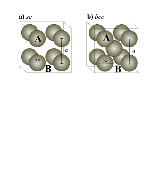
Let’s consider an ideal periodic structure consisting of spheres of ferromagnetic A and embedded in a matrix of ferromagnetic B. The spheres are assumed to form a 3D periodical lattice of $sc$ (Fig. 1a) or bcc (Fig. 1b) type. A static magnetic field, $H_{0}$, is applied to the composite along the $x_{3}$ axis, and assumed to be strong enough to saturate the magnetization of both materials. The lattice constant is denoted by $a$; the filling fraction, $f$, is defined as the volume proportion of material A in a unit cell:

$$f={\displaystyle\frac{\frac{4}{3}\pi R^{3}}{a^{3}}}\;\;\;\mbox{({\em sc})}\;\;\;\;\;\mbox{or}\;\;\;\;\;f={\displaystyle\frac{\frac{8}{3}\pi R^{3}}{a^{3}}}\;\;\;\mbox{({\em bcc}),}$$ (1)

in an sc or bcc lattice, respectively.

Figure 1: The 3D periodic structures studied in this paper; two types of structure are considered, both consisting of ferromagnetic spheres of material A embedded in a matrix of material B (materials A and B have different magnetic properties); (a) the spheres are disposed in the nodes of an sc lattice; (b) the spheres are disposed in the nodes of a bcc lattice.

Ferromagnetics A and B are characterized by two material parameters: the spontaneous magnetization ($M_{S,A}$ and $M_{S,B}$), and the exchange constant ($A_{A}$ and $A_{B}$); both these parameters depend on the position vector $\vec{r}=(x_{1},x_{2},x_{3})$:

$$M_{S}(\vec{r}) = M_{S,B}+(M_{S,A}-M_{S,B})S(\vec{r}),$$

$$A(\vec{r}) = A_{B}+(A_{A}-A_{B})S(\vec{r}),$$ (2)

the value of function $S(\vec{r})$ being 1 inside a sphere, and 0 beyond.

In the classical approximation, spin waves are described by the Landau-Lifshitz (LL) equation, taking the following form in the case of magnetic composites (with damping neglected):

$$\frac{\partial\vec{M}(\vec{r},t)}{\partial t}=\gamma\mu_{0}\vec{M}(\vec{r},t)\times\vec{H}_{eff}(\vec{r},t),$$ (3)

where magnetization $\vec{M}(\vec{r},t)$ is a function of position vector $\vec{r}$ and time $t$;
$\vec{H}_{eff}(\vec{r},t)$ stands for the effective magnetic field acting on magnetization $\vec{M}(\vec{r},t)$ and defined as follows [17] -[19] :

$$\vec{H}_{eff}(\vec{r},t)=H_{0}\vec{e}_{3}+\vec{h}(\vec{r},t)+\frac{2}{\mu_{0}}\left(\nabla\cdot\frac{A}{M^{2}_{S}}\nabla\right)\vec{M}(\vec{r},t);$$ (4)

$\vec{e}_{i}$ is the unit vector along the $x_{i}$ axis; $\vec{h}(\vec{r},t)$ is the dynamic magnetic field due to dipolar interactions; the third component represents the exchange field. The magnetization vector can be represented as the sum of its static component, $M_{S}\vec{e}_{3}$, which is parallel to the applied field, and its dynamic component, $\vec{m}(\vec{r},t)$, lying in plane ($x_{1},x_{2}$):

$$\vec{M}(\vec{r},t)=M_{S}\vec{e}_{3}+\vec{m}(\vec{r},t).$$ (5)

The dynamic dipolar field, $\vec{h}$, must satisfy the magnetostatic Maxwell equations:

$$\nabla\times\vec{h}(\vec{r})=0,$$

$$\nabla\cdot\left(\vec{h}(\vec{r})+\vec{m}(\vec{r})\right)=0.$$ (6)

In magnonic crystals, the position-dependent coefficients in (3), i.e. $M_{S}$ and $A$, are periodic functions of the position vector, which allows us to use, in the procedure of solving the LL equation defined in (3), the plane wave method, described in detail in our earlier papers [17] ; [18] (dealing with two-dimensional magnonic crystals). Following this scheme, we proceed to Fourier-expanding all the periodic functions of the position vector, i.e. the spontaneous magnetization, $M_{S}$, and parameter $Q$ defined as follows:

$$Q=\frac{2A}{\mu_{0}M^{2}_{S}H_{0}}.$$ (7)

The dynamic components of the magnetization can be expressed as the product of the periodic envelope function and the Bloch factor $exp(i\vec{K}\vec{r}$) ($\vec{K}$ denoting a 3D wave vector); the envelope function can be transformed into the reciprocal space as well. Including all the expansions into (4) and (6) leads to the following infinite system of linear equations for Fourier coefficients of the dynamic magnetization components, $\vec{m}_{1\vec{k}}(\vec{g})$ and $\vec{m}_{2\vec{k}}(\vec{g})$:

$$i\Omega m_{1\vec{k}}(\vec{g}) = m_{2\vec{k}}(\vec{g})+\frac{1}{H_{0}}\sum_{\vec{g}^{\prime}}\frac{(k_{2}+g^{\prime}_{2})(k_{1}+g^{\prime}_{1})}{|\vec{k}+\vec{g}^{\prime}|^{2}}m_{1\vec{k}}(\vec{g}^{\prime})M_{S}(\frac{2\pi}{a}(\vec{g}-\vec{g}^{\prime}))$$

$$+ \frac{1}{H_{0}}\sum_{\vec{g}^{\prime}}\frac{(k_{2}+g^{\prime}_{2})^{2}}{|\vec{k}+\vec{g}^{\prime}|^{2}}m_{2\vec{k}}(\vec{g}^{\prime})M_{S}(\frac{2\pi}{a}(\vec{g}-\vec{g}^{\prime}))$$

$$+ \sum_{\vec{g}^{\prime}}\sum_{\vec{g}^{\prime\prime}}\left(\frac{2\pi}{a}\right)^{2}[(\vec{k}+\vec{g}^{\prime})\cdot(\vec{k}+\vec{g}^{\prime\prime})-(\vec{g}-\vec{g}^{\prime\prime})\cdot(\vec{g}-\vec{g}^{\prime})]$$

$$\cdot M_{S}(\frac{2\pi}{a}(\vec{g}-\vec{g}^{\prime\prime}))Q(\frac{2\pi}{a}(\vec{g}^{\prime\prime}-\vec{g}^{\prime}))m_{2\vec{k}}(\vec{g}^{\prime}),$$

$$i\Omega m_{2\vec{k}}(\vec{g}) = -m_{1\vec{k}}(\vec{g})+-\frac{1}{H_{0}}\sum_{\vec{g}^{\prime}}\frac{(k_{2}+g^{\prime}_{2})(k_{1}+g^{\prime}_{1})}{|\vec{k}+\vec{g}^{\prime}|^{2}}m_{2\vec{k}}(\vec{g}^{\prime})M_{S}(\frac{2\pi}{a}(\vec{g}-\vec{g}^{\prime}))$$ (8)

$$- \frac{1}{H_{0}}\sum_{\vec{g}^{\prime}}\frac{(k_{1}+g^{\prime}_{1})^{2}}{|\vec{k}+\vec{g}^{\prime}|^{2}}m_{1\vec{k}}(\vec{g}^{\prime})M_{S}(\frac{2\pi}{a}(\vec{g}-\vec{g}^{\prime}))$$

$$- \sum_{\vec{g}^{\prime}}\sum_{\vec{g}^{\prime\prime}}\left(\frac{2\pi}{a}\right)^{2}[(\vec{k}+\vec{g}^{\prime})\cdot(\vec{k}+\vec{g}^{\prime\prime})-(\vec{g}-\vec{g}^{\prime\prime})\cdot(\vec{g}-\vec{g}^{\prime})]$$

$$\cdot M_{S}(\frac{2\pi}{a}(\vec{g}-\vec{g}^{\prime\prime}))Q(\frac{2\pi}{a}(\vec{g}^{\prime\prime}-\vec{g}^{\prime}))m_{1\vec{k}}(\vec{g}^{\prime}).$$

$\vec{k}_{i}$ and $\vec{g}_{i}$ denoting the Cartesian components of a dimensionless wave vector $\vec{k}=(a/2\pi)\vec{K}$ and a dimensionless reciprocal lattice vector $\vec{g}=(a/2\pi)\vec{G}$, respectively; a new quantity introduced in (8) is $\Omega$, henceforth referred to as reduced frequency:

$$\Omega=\frac{\omega}{|\gamma|\mu_{0}H_{0}}.$$ (9)

The Fourier coefficients of spontaneous magnetization $M_{S}$ and parameter $Q$ are calculated from the inverse Fourier transformation; in the case of spheres the resulting formulae read as follows:

$$M_{S}(\vec{G})=\left\{\begin{array}[]{ll}M_{S,A}f+M_{S,B}(1-f),&\;\;\mbox{for $\;\vec{G}=0$}\\ &\\ f(M_{S,A}-M_{S,B}){\displaystyle\frac{3\left[\sin(GR)-(GR)\cos(GR)\right]}{(GR)^{3}}},&\;\;\mbox{for $\;\vec{G}\neq 0$}\end{array}\right.,$$ (13)

and similarly

$$Q(\vec{G})=\left\{\begin{array}[]{ll}Q_{A}f+Q_{B}(1-f),&\;\;\mbox{for $\;\vec{G}=0$}\\ &\\ f(Q_{A}-Q_{B}){\displaystyle\frac{3\left[\sin{(GR)}-(GR)\cos(GR)\right]}{(GR)^{3}}},&\;\;\mbox{for $\;\vec{G}\neq 0$}\end{array}\right.,$$ (17)

where $Q_{A}$ and $Q_{B}$ are the values of parameter $Q$ in material A and B, respectively; $R$ is the sphere radius (Fig. 1).

Obviously, the numerical calculations performed on the basis of (8) involve a finite number of reciprocal lattice vectors $\vec{G}$ in the Fourier expansions; however, we have made sure that the number used is large enough to ensure good convergence of the numerical results. As indicated by an analysis performed, a satisfactory convergence is obtained already with 343 reciprocal lattice vectors used.

Figure 2: . The Brillouin zones corresponding to the considered structures, and the paths (highlighted) along which the magnonic band structures are calculated: (a) $M\Gamma XMR$ in the case of the $sc$ lattice, (b) $P\Gamma HNP$ in the case of the $bcc$ lattice.

III Numerical results

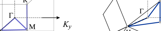
The first 3D magnonic crystal to be studied here is a magnetic composite consisting of ferromagnetic spheres (of material A) disposed in the nodes of a simple cubic (sc) lattice and embedded in a different magnetic material (B), referred to as matrix (Fig. 1a). The corresponding magnonic band structure will be calculated along path $M=\pi/a(1,1,0)\rightarrow\Gamma=\pi/a(0,0,0)\rightarrow X=\pi/a(1,0,0)\rightarrow M=\pi/a(1,1,0)\rightarrow R=\pi/a(1,1,1)$ in the nonreducible part of the first Brillouin zone (see Fig. 2a). Iron and yttrium iron garnet (YIG) are chosen as component materials A (spheres) and B (matrix), respectively, in the studied example. As established in our earlier studies [17] ; [18] , in the case of 2D magnonic crystals, such composition, involving a substantial contrast of the magnetic parameters between the component materials ($M_{S,Fe}=1.752\;10^{6}Am^{-1}$, $M_{S,YIG}=0.194\;10^{6}Am^{-1}$, $A_{Fe}=2.1\;10^{-11}Jm^{-1}$, $A_{YIG}=0.4\;10^{-11}Jm^{-1}$), leads to large energy gaps in the spin wave spectrum. Also in the spin wave spectrum obtained for the sc lattice-based 3D magnonic crystal considered here, two wide energy gaps are present, one between bands 1 and 2, the other between bands 5 and 6, as shown in Fig. 3. The existence of these gaps signifies that spin waves having frequency values within a gap cannot propagate in the composite. The following parameter values have been assumed in our calculations: crystal lattice constant $a$=100$\AA$, applied static magnetic field $\mu_{0}H_{0}=0.1$T, and filling fraction $f$=0.2.

Figure 3: The magnonic band structure found numerically for the $sc$ lattice-based composite (iron spheres embedded in a YIG matrix). The spin wave energy branches have been calculated along the path (in the first Brillouin zone) shown in Fig. 2a. The following parameter values are assumed: applied static magnetic field $\mu_{0}H_{0}=0.1$T, crystal lattice constant $a=100\AA$, and filling fraction $f$=0.2.

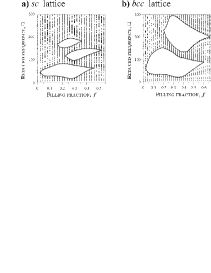
Let’s examine the effect of the filling fraction on the width of the gaps obtained. Figure 4a shows the magnonic bands plotted against the filling fraction in the sc lattice-based structure ($Fe$ spheres embedded in YIG); the plot was obtained through projecting the magnonic band structure calculated along $M\Gamma XMR$ (for a fixed filling fraction value) on the reduced frequency ($\Omega$) axis; the procedure of projection was performed repeatedly for consecutive filling fraction values. The first (lowest) gap shown in Fig. 4a is found to be the largest for filling fraction value $f$=0.24, the corresponding gap width being $\Delta\Omega$=63.29, while the much narrower second gap reaches its maximum width at $f$=0.3. Unlike in 1D and 2D magnonic crystals, no oscillatory variations of the energy gaps with the filling fraction are observed in the 3D composites [17] ; [18] ; [22] . The gaps found in the bcc lattice-based structure, shown in Fig. 4b, are clearly much broader than those in the sc lattice-based structure. The spin wave reduced frequency was calculated along path $P\Gamma HNP$ [$P=\pi/a(1,1,1)\rightarrow\Gamma=\pi/a(0,0,0)\rightarrow H=\pi/a(2,0,0)\rightarrow N=\pi/a(1,1,0)\rightarrow P=\pi/a(1,1,1)$] (indicated by a bold line in Fig. 2b) in the bcc lattice first Brillouin zone. The maximum width of the first gap is found to occur at $f$=0.2, reaching value $\Delta\Omega$=117.02, which is 85% larger than its counterpart in the sc lattice-based structure. The second energy gap found in the bcc lattice-based structure (between bands 4 and 5) is broader than the first one, and reaches a maximum width of $\Delta\Omega$ =141.52 at filling fraction value $f$=0.32.

Figure 4: The magnonic energy branches in cubic magnonic crystals ($Fe$ spheres embedded in YIG) plotted versus the filling fraction (a) for an $sc$ lattice-based structure, and (b) for a $bcc$ lattice-based structure. The lattice constant value is assumed to be $a=100\AA$, and the applied magnetic field value to be $\mu_{0}H_{0}=0.1$T.

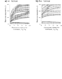
Let’s proceed now to the role played by the magnetic parameters of the component materials. Figure 5 shows spin wave energy branches plotted against the contrast between the spontaneous magnetization values in materials A (spheres) and B (matrix); this contrast, defined as ratio $M_{S,A}/M_{S,B}$, will be henceforth shortly referred to as magnetization contrast. The computations have been performed for a fictitious matrix material whose spontaneous magnetization and exchange constant values, $M_{S,B}$ and $A_{B}$, respectively, are fixed at values close to those in YIG; the exchange constant value in the sphere material is assumed to be $A_{A}=2.1\;10^{-11}Jm^{-1}$. The other parameters are fixed as well: the assumed lattice constant value is $a$=100$\AA$, the filling fraction $f$=0.2, and the applied magnetic field $\mu_{0}H_{0}=0.1$T. The results obtained for the sc lattice-based and the bcc lattice-based structures are depicted in Figs. 5a and 5b, respectively. Let’s focus on the first gap occurring between the first and the second energy bands; the gap width is found to be maximal for magnetization contrast values 10 and 12.8 in the bcc lattice-based and the sc lattice-based structures, respectively. Both these values are not far from the spontaneous magnetization contrast between iron and YIG ($M_{S,Fe}/M_{S,YIG}$ = 10.82), the material composition used in the above-discussed investigation of the effect of the filling fraction, and leading to quite wide gaps, as one can see in Figs. 4a and 4b. Note that in both lattice types the minimum spontaneous magnetization contrast necessary for energy gaps to open is greater than 2.

Figure 5: Three-dimensional magnonic crystal spin wave spectra plotted versus the magnetization contrast, on the basis of computations performed for (a) an $sc$ lattice-based structure, and (b) a $bcc$ lattice-based structure. The assumed spontaneous magnetization and exchange constant values in the matrix are $M_{S,B}=0.194\;10^{6}Am^{-1}$ and $A_{B}=0.4\;10^{-11}Jm^{-1}$, close to the respective parameter values in YIG; the exchange constant value in the spheres is assumed to be $A_{A}=2.1\;10^{-11}Jm^{-1}$, the lattice constant $a=100\AA$, the filling fraction $f=0.2$, and the applied field $\mu_{0}H_{0}=0.1T$.

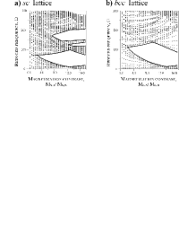
In the last stage of this investigation, we shall examine the role of the contrast between the exchange constant values in the component materials. The results of the respective computations are depicted in Fig. 6, showing magnonic branches versus the exchange contrast, defined as the ratio ($A_{A}/A_{B}$) between the exchange constant values in materials A (spheres) and B (matrix); results obtained for sc and bcc lattice-based structures are shown in Figs. 6a and 6b, respectively. The only variable in the computations was the exchange constant in material A, all the other structural and material parameters being fixed: $M_{S,A}=1.752\;10^{6}Am^{-1}$, $M_{S,B}=0.194\;10^{6}Am^{-1}$, $A_{B}=0.4\;10^{-11}Jm^{-1}$, $a=100\AA$, $\mu_{0}H_{0}=0.1$T. The occurrence of the first energy gap (between the first and the second magnonic bands) is found to be independent of the exchange contrast, yet the gap width grows as the exchange contrast increases. This means that the exchange contrast is not an indispensable factor for the opening of complete energy gaps in 3D magnonic crystals, its effect being limited to the width of the existing gaps.

Figure 6: Magnonic branches plotted versus the exchange contrast in the composite. The assumed values of the matrix material parameters are close to the respective parameter values in YIG; the spontaneous magnetization in the spheres is assumed to be $M_{S,A}=2.1\;10^{6}Am^{-1}$. Other parameter values are as in Fig. 5.

IV Confrontation of the theory with the experiment

As demonstrated by the above-presented results, complete energy gaps can occur in the spin wave spectra of 3D periodic magnetic composites. The opening of such gaps is conditioned on the material composition, as gaps are found to exist only when the spontaneous magnetization contrast is greater than 2. The gap width can be controlled through adjusting the filling fraction value, and the position of the gap on the energy scale through modifying the value of the applied magnetic field. As expected, the bcc lattice-based structure is found to give rise to larger energy gaps than the sc lattice-based one.

Figure 7: Magnonic band structure computed on the basis of Eqs (8) for a hypothetic periodic structure of ferromagnetic droplets existing in doped manganites $La_{1-x}Ca_{x}MnO_{3}$ $(1\%<x<9\%)$; the droplets are assumed to be sphere-shaped and to form a regular crystal lattice of $bcc$ type. The material and structural parameter values used in the computations are as follows: $M_{S,A}=0.8\;10^{6}Am^{-1}$, $M_{S,B}=0.2\;10^{6}Am^{-1}$, $A_{A}=0.04\;10^{-11}Jm^{-1}$, $A_{B}=0.02\;10^{-11}Jm^{-1}$, $f=0.25$, $a=50\AA$, $\mu_{0}H_{0}=0.1T$, close to the respective estimate values obtained experimentally [32] .

We shall try to confront our theory with available experimental results now. Energy gaps have recently been found in spin wave spectra of doped manganites $La_{1-x}Ca_{x}MnO_{3}$ and $La_{1-x}Sr_{x}MnO_{3}$ at low concentrations ($2\%<x<9\%$) of $Ca$ and $Sr$ ions [32] -[35] . The quoted studies demonstrated the existence of ferromagnetic nanoregions (referred to as droplets) in these materials at temperatures below a critical point; the space between the droplets is filled with a different magnetic (ferromagnetic or antiferromagnetic) medium. We suggest that the spin wave spectrum gap recently found experimentally through neutron scattering on doped manganites might be an indirect indication of periodic spatial distribution of the ferromagnetic droplets. Assuming that the droplets (material A) are sphere-shaped and disposed in the nodes of a bcc lattice, we have computed the magnonic spectrum in a 3D composite with structural and material parameter values close to those reported in the experimental studies [32] -[35] . The resulting spin wave spectrum is shown in Fig. 7; the following parameter values are assumed: $M_{S,A}=0.8\;10^{6}Am^{-1}$, $M_{S,B}=0.2\;10^{6}Am^{-1}$, $A_{A}=0.04\;10^{-11}Jm^{-1}$, $A_{B}=0.02\;10^{-11}Jm^{-1}$, $f=0.25$, $a=50\AA$, $\mu_{0}H_{0}=0.1$T. A narrow energy gap is found in the obtained spectrum (between the first and the second bands), in the same frequency range as the gap which was found in the neutron scattering experiments [32] -[35] . The gap resulting from our numerical computations lies between 1.27meV and 1.49meV; the gap found experimentally had width 0.2meV and was reported to lie in the vicinity of 1.65meV. As the ”computed” gap has width 0.22meV, the result obtained on the ground of our theory can be deemed close to the experimental one. This preliminary result fills us with optimism, as it allows us to propose a working hypothesis supposing that the manganites in question can be regarded as 3D manganite structures. This, however, will remain unconfirmed as long as no direct experimental evidence of the regularity of the structure formed by the droplets is available (cf. results reported in [36] ). We shall continue our research in order to find further evidence supporting our hypothesis.

Acknowledgements

The present work was supported by the Polish State Committee for Scientific Research through projects KBN - 2P03B 120 23 and PBZ-KBN-044/P03-2001.

References

- (1) E. Yablonovitch, Phys. Rev. Lett. 58 (1987) 2059
- (2) S. John, Phys. Rev. Lett. 58 (1987) 2486
- (3) Development and Applications of Materials Exhibiting Photonic Gaps, Eds. C. M. Bowden, J. P. Dowling, H. O. Everitt, J. Opt. Soc. Am. B 10 (1993) 280
- (4) J. D. Joannopoulos, R. D. Meade, J. N. Winn, Photonic Crystals (Princeton Univ. Press, Princeton, NJ, 1995)
- (5) K. Sakoda, Optical Properties of Photonic Crystals (Springer, Berlin, 2001)
- (6) J. B. Pendry, Phys. Rev. Lett. 85 (2000) 3966
- (7) J. B. Pendry, D. R. Smith, Physics Today 57 (June 2004) 37
- (8) M. S. Kushwaha, P. Halevi, L. Dobrzynski, B. Djafari-Rouhani, Phys. Rev. Lett. 71 (1993) 2022
- (9) M. M. Sigalas, E. N. Economou, Solid State Commun. 86 (1993) 141
- (10) Y. Lai, Z.-Q. Zhang, Appl. Phys. Lett. 83 (2003) 3900
- (11) M. M. Sigalas, C. M. Soukoulis, R. Biswas, K. M. Ho, Phys. Rev. B 56 (1997) 959
- (12) A. Saib, D. Vanhoenacker-Janvier, I. Huynen, A. Encinas, L. Piraux, E. Ferain, R. Legras, Appl. Phys. Lett. 83 (2003) 2378
- (13) Z. Lin, S. T. Chui, Phys. Rev. E 69 (2004) 056614
- (14) P. Xu, T.-Y. Cai, Z.-Y. Li, Solid State Communications 130 (2004) 451
- (15) S.A. Nikitov, Ph. Tailhades, Optics Communications 199 (2001) 389
- (16) J. O. Vasseur, L. Dobrzynski, B. Djafari-Rouhani, H. Puszkarski, Phys. Rev. B 54 (1996) 1043
- (17) M. Krawczyk, H. Puszkarski, Acta Physica Polonica A 93 (1998) 805
- (18) M. Krawczyk, H. Puszkarski, Acta Physicae Superficierum 3 (1999) 89
- (19) H. Puszkarski, M. Krawczyk, Solid State Phenomena 94 (2003) 125
- (20) Y.V. Gulyaev, S.A. Nikitov, L.V. Zhivotovskii, A.A Klimov, P. Tailhades, L. Presmanes, C. Bonningue, C.S. Tsai, S.L. Vysotskii, Y.A.Filimonov, J.E.T.P. Letters 77 (2003) 670
- (21) M. Shamonin, A. Snarskii and M. Zhenirovskiyy, NDT&E International 37 (2004) 35
- (22) A. Akjouj, A. Mir, B. Djafari-Rouhani, J.O. Vasseur, L. Dobrzynski, H. Al Wahsh, P.A. Deymier, Surface Science 482 (2001) 1062
- (23) A. Mir, H. Al Wahsh, A. Akjouj, B. Djafari-Rouhani, L. Dobrzynski, J.O. Vasseur, J. Phys.: Condens. Matter 14 (2002) 637
- (24) H. Puszkarski, M. Krawczyk, Physics Letters A 282 (2001) 106
- (25) H. Puszkarski, M. Krawczyk, J.-C. S. Levy, D. Mercier, Acta Physica Polonica A 100 (Supplement) (2001) 195
- (26) S.A. Nikitov, Ph. Tailhades, C.S. Tsai, J. Magn. Magn. Mater. 236 (2001) 320
- (27) H. Al-Wahsh, Phys. Rev. B 69 (2004) 012405
- (28) V.V. Kruglyak, A.N. Kuchko, The Physics of Metals and Metallography 93 (2002) 511
- (29) V.V. Kruglyak, A.N. Kuchko, Physica B 339 (2003) 130
- (30) V.V. Kruglyak, A.N. Kuchko, J. Magn. Magn. Mater. 272-276 (2004) 302
- (31) R. Seshadri, R.M. Weservelt, Phys. Rev. B 47 (1993) 8620
- (32) M. Hennion, F. Moussa, J. Rodr guez-Carvajal, L. Pinsard, A. Revcolevschi, Phys. Rev. Lett. 81 (1998) 1957
- (33) F. Moussa, M. Hennion, G. Biotteau, J. Rodri guez-Carvajal, L. Pinsard, A. Revcolevschi, Phys. Rev. B 60 (1999) 12299
- (34) G. Biotteau, M. Hennion, F. Moussa, J. Rodri guez-Carvajal, L. Pinsard, A. Revcolevschi, Y. M. Mukovskii, D. Shulyatev, Phys. Rev. B 64 (2001) 104421
- (35) F. Moussa, M. Hennion, F. Wang, P. Kober, J. Rodri guez-Carvajal, P. Reutler, L. Pinsard, A. Revcolevschi, Phys. Rev. B 67 (2003) 214430
- (36) P.A. Algarabel, J.M. De Teresa, J. Blasco, M.R. Ibrra, Cz. Kapusta, M. Sikora, D. Zaja̧c, P.C. Riedi, C. Ritter, Phys. Rev. B 67 (2003) 134402