Asymmetry of magnetic-field profiles in superconducting strips

Abstract

We analyze the magnetic-field profiles $H_{z}(x)$ at the upper (lower) surface of a superconducting strip in an external magnetic field, with $z$ perpendicular to the plane of the strip and $x$ along its width. The external magnetic field $H_{a}$ is perpendicular or inclined to the plane of the strip. We show that an asymmetry of the profiles $H_{z}(x)$ appears in an oblique magnetic field $H_{a}$ and also in the case when the angular dependence of the critical current density $j_{c}$ in the superconductor is not symmetric relative to the $z$ axis. The asymmetry of the profiles is related to the difference $\Delta H_{z}(x)$ of the magnetic fields at the upper and lower surfaces of the strip, which we calculate. Measurement of this difference or, equivalently, of the asymmetry of the profiles can be used as a new tool for investigation of flux-line pinning in superconductors.

I Introduction

In a recent Letter t magnetic-field profiles at the upper surface of a thin rectangular YBa₂Cu₃O_7-δ platelet placed in a perpendicular external magnetic field were investigated by magneto-optical imaging, and the following interesting observation was made: When columnar defects slightly tilted to the c-axis (normal to the platelet surface) were introduced into the sample by heavy-ion irradiation, an asymmetry of the magnetic-field profiles relative to the central axis of the sample appeared, and this asymmetry nonmonotonically depended on the magnitude of the external magnetic field $H_{a}$, disappearing at large $H_{a}$. The authors of Ref. t, explained the asymmetry by in-plane magnetization originating from a zigzag structure of vortices, i.e., from their partial alignment along the columnar defects. They also implied that when the vortices lose their interlayer coherence, the in-plane magnetization and hence the asymmetry disappear. On this basis, it was claimed t that the asymmetry can be a powerful probe for the interlayer coherence in superconductors. In this paper we show that the asymmetry of the magnetic field profiles in thin flat superconductors may have a more general origin. It may result from anisotropy of flux-line pinning and needs not be due to the kinked structure of vortices. The asymmetry can occur not only in layered superconductors but also in three dimensional materials, and its disappearance can be understood without the assumption that the interlayer coherence is lost. Interestingly, without any columnar defects, such an asymmetry of the magnetic field profiles was recently observed in a Nb₃Sn slab placed in an oblique magnetic field. w

In Ref. 1, ; obl1, we explained how to solve the critical state problem for thin flat three-dimensional superconductors with an arbitrary anisotropy of flux-line pinning. But these equations yield magnetic-field profiles in the critical state only to the leading order in the small parameter $d/w$ where $d$ is the thickness of the flat superconductor and $w$ is its characteristic lateral dimension. In this approximation the magnetic-field component perpendicular to the flat surfaces of the sample, $H_{z}$, is independent of the coordinate $z$ across the thickness of the superconductor and coincides with the appropriate magnetic field of an infinitely thin superconductor of the same shape (but with some dependence of the critical sheet current $J_{c}$ on $H_{z}$). As it will be seen below, the asymmetry of the profiles is related to the difference $\Delta H_{z}$ of the fields $H_{z}$ at the upper and lower surfaces of the sample. Thus, to describe the asymmetry of the $H_{z}$ profiles, it is necessary to consider these profiles more precisely, to the next order in $d/w$, taking into account the dependence of $H_{z}$ on the coordinate across the thickness of the superconductor.

In this paper we obtain formulas for $\Delta H_{z}$ and for the asymmetry of the magnetic-field profiles in an infinitely long thin strip, and discuss the conditions under which the asymmetry can be observed. In particular, an asymmetry always will appear for strips in an oblique magnetic field, and experimental investigation of this asymmetry provides new possibilities for analyzing flux-line pinning in superconductors. We also demonstrate that the experimental data of Ref. t, can be qualitatively understood by assuming some anisotropy of pinning in a three-dimensional (not layered) superconductor.

II Magnetic-field profiles of strips

In this paper we consider the following situation: A thin three dimensional superconducting strip fills the space $|x|\leq w$, $|y|<\infty$, $|z|\leq d/2$ with $d\ll w$; a constant and homogeneous external magnetic field $H_{a}$ is applied at an angle $\theta_{0}$ to the $z$ axis ($H_{ax}=H_{a}\sin\theta_{0}$, $H_{ay}=0$, $H_{az}=H_{a}\cos\theta_{0}$). For definiteness, we shall imply below that $H_{ax}$ is switched on first and then $H_{az}$ is applied, i.e., the so-called third scenario obl1 of switching on $H_{a}$ occurs (for the definition of the first and second scenarios see Appendix B). It is also assumed that surface pinning is negligible, the thickness of the strip, $d$, exceeds the London penetration depth, and the lower critical field $H_{c1}$ is sufficiently small so that we may put $B=\mu_{0}H$.

The symmetry of the problem leads to the following relationships:

$$j_{y}(x,z)=-j_{y}(-x,-z),$$

$$H_{z}(x,z)=H_{z}(-x,-z),\ \ \ H_{x}(x,z)=H_{x}(-x,-z),$$

where $j_{y}(x,z)$ is the current density flowing at the point ($x$,$z$). In other words, the field at the lower surface of the strip, $H_{z}^{-}(x)\equiv H_{z}(x,-d/2)$, can be expressed via the field at its upper surface, $H_{z}^{+}(x)\equiv H_{z}(x,d/2)$, as follows:

$$H_{z}^{-}(x)=H_{z}^{+}(-x),$$

and hence for the difference $\Delta H_{z}(x)\equiv H_{z}^{+}(x)-H_{z}^{-}(x)$ of the fields at the upper and lower surfaces we obtain the formula

$$\Delta H_{z}(x)=H_{z}^{+}(x)-H_{z}^{+}(-x),$$ (1)

which connects this $\Delta H_{z}(x)$ and the asymmetry of the magnetic-field profile at the upper surface of the strip.

As mentioned in the Introduction, to leading order in $d/w$ the critical state problem for such a strip can be reduced to the critical state problem for the infinitely thin strip with some dependence of the critical sheet current $J_{c}$ on $H_{z}$ where the sheet current is the current density integrated over the thickness of the strip,

$$J\equiv\int_{-d/2}^{d/2}j_{y}(x,z)dz,$$

and $J_{c}$ is its critical value. The dependence $J_{c}(H_{z})$ results from both a dependence of the critical current density $j_{c}$ on the absolute value of the local magnetic induction $\mu_{0}|H|$ and an out-of-plane anisotropy of $j_{c}$, i.e., a dependence of $j_{c}$ on the angle $\theta$ between the local direction of ${\bf H}$ and the $z$ axis. Since both $|H|$ and $\theta$ change with $z$ in strips of finite thickness, this means that $J_{c}\neq j_{c}d$, and a dependence of $J_{c}$ on $H_{z}$ appears. The function $J_{c}(H_{z})$ can be found from the equation, 1 ; obl1

$$d=\!\!\int_{H_{x}^{-}}^{H_{x}^{+}}\!\!{dh\over j_{c}(h,H_{z})},$$ (2)

where the critical current density $j_{c}(H_{x},H_{z})$ may have arbitrary dependence on the local $H_{x}$ and $H_{z}$; $H_{x}^{-}=H_{ax}-0.5J_{c}(H_{z})$, and $H_{x}^{+}=H_{ax}+0.5J_{c}(H_{z})$ are the $x$ component of the magnetic field at the lower and the upper surfaces of the strip. The function $J_{c}(H_{z})$ found from Eq. (2) generally depends on the parameter $H_{ax}$, and only within the Bean model when $j_{c}$ is independent of ${\bf H}$, equation (2) yields $J_{c}=j_{c}d$ for any $H_{ax}$.

Formula (2) is valid to the leading order in $d/w$ since we neglected the term $\partial H_{z}(x,z)/\partial x$ in the equation ${\rm rot}{\bf H}={\bf j}$ and used the expression

$${\partial H_{x}(x,z)\over\partial z}=j_{y}(x,z)$$ (3)

with $j_{y}(x,z)=j_{c}(H_{x},H_{z})$ to derive formula (2). In this approximation $H_{z}$ is independent of $z$ inside the strip. Thus $\Delta H_{z}(x)=0$, and so the $H_{z}$ profile is always symmetric. This profile is given by the Biot-Savart law for the infinitely thin strip

$$H_{z}(x)=H_{az}+{1\over 2\pi}\!\int_{-w}^{w}\!\!{J(t)\,dt\over t-x}\,.$$ (4)

Here the sheet current $J(x)$ follows from the critical state equations for this strip:

$$J(x)=-{x\over|x|}J_{c}[H_{z}(x)]$$ (5)

if $a\leq|x|\leq w$, and

$$H_{z}(x)=0$$ (6)

when $|x|\leq a$. The points $x=\pm a$ give the position of the flux front in the infinitely thin strip. The integral equations (4) - (6) can be solved by either a static iterative method, or more conveniently by a dynamic method. EH ; EH1

An analysis of $H_{z}$ allowing for terms of the order of $d/w$ is presented in Appendix A. In this case $\Delta H_{z}\neq 0$, and it is given by

$$\Delta H_{z}(x)={d\over dx}\int_{-d/2}^{d/2}zj_{y}(x,z)dz\,.$$ (7)

This expression can be also derived from the following simple considerations: Using ${\rm div}{\bf H}=0$, we write

$$\Delta H_{z}(x)=\!\!\int_{-d/2}^{d/2}\!\!{\partial H_{z}(x,z)\over\partial z}dz=-\!\!\int_{-d/2}^{d/2}\!\!{\partial H_{x}(x,z)\over\partial x}dz.$$ (8)

From Eq. (3) it follows that

$$H_{x}(x,z)=H_{x}(x,-d/2)+\int_{-d/2}^{z}j_{y}(x,z^{\prime})dz^{\prime}.$$

Inserting this expression into formula (8), interchanging the sequence of the integrations, and using $H_{x}(x,-d/2)=H_{ax}-0.5J(x)$, we find formula (7). It follows from this formula that an asymmetry of the $H_{z}$-profile can appear only if the distribution of the current density $j_{y}$ across the thickness of the strip is asymmetric about the middle plane of the strip, $z=0$, and if this distribution changes with $x$ (the latter condition was not obtained in Ref. t, ). c1

III Conditions for asymmetry

If the angular dependence of the critical current density is symmetric relative to the $z$ axis, $j_{c}(-H_{x},H_{z})=j_{c}(H_{x},H_{z})$, an asymmetry of the current distribution across the thickness of the strip can occur only in an oblique applied magnetic field which breaks the relation $H_{x}(x,-z)=-H_{x}(x,z)$. Besides this, asymmetry of the distribution can appear for asymmetric angular dependence of $j_{c}$, $j_{c}(-H_{x},H_{z})\neq j_{c}(H_{x},H_{z})$, even when the external magnetic field is applied along the $z$ axis. In this section we consider the case of an oblique magnetic field.

III.1 Region where $H_{z}\approx 0$

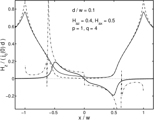
For a superconducting strip in an oblique magnetic field, it was shown recently mbi that in the region of the strip, $|x|\leq a$, where a flux-free core occurs, i.e., where $H_{z}\approx 0$, the distribution of the current across the thickness of the sample is highly asymmetric even for superconductors with ${\bf H}$-independent $j_{c}$ (the Bean model). Using this distribution (which depends on how the magnetic field is switched on) and Eq. (7), one can calculate $\Delta H_{z}(x)$ in this region of the strip. Note that the results of such calculations may be also applied to anisotropic strips with $j_{c}=j_{c}(\theta)$ since in this region of the strip the flux lines practically lie in the $x$-$y$ plane, $j_{c}$ is independent of the coordinates, $j_{c}\approx j_{c}(\pi/2)$, and the results for the flux-free core obtained within the Bean model remain applicable to this anisotropic case. In Fig. 1 we present this $\Delta H_{z}(x)$ for the anisotropic strip in the case of the third scenario obl1 of switching on $H_{a}$ when the field $H_{ax}$ is switched on first and then the component $H_{az}$ is applied, see Appendix B. Thus, a nonzero $\Delta H_{z}$ in this region of the sample reflects the asymmetry of the flux-free core, and this $\Delta H_{z}$ differs from zero in an oblique magnetic field for any superconductor.

The quantity $\Delta H_{z}(x)$ in the region $|x|<a$ depends on how the external magnetic field is switched on. In particular, when $H_{ax}$ is applied before $H_{az}$ (the third scenario) and $j_{c}d/2<H_{ax}$, $\Delta H_{z}(x)$ is described by Eq. (B9). On the other hand, for the same applied field but with $H_{ax}$ and $H_{az}$ switched on simultaneously (the so-called first scenario mbi ), we obtain from formulas of Ref. mbi, at $|x|<a\sin\theta_{0}$

$$\Delta H_{z}(x)=-{J(x)\over 2j_{c}}{dJ(x)\over dx}.$$ (9)

Comparison of Eqs. (B9) and (9) demonstrates that measurements of the asymmetry of the $H_{z}$ profiles at the upper surface of the strip enable one to investigate subtle differences between critical states generated by different scenarios of switching on $H_{a}$ (to the leading order in the small parameter $d/w$ one has $H_{z}=0$ at $|x|<a$ for any scenario). Note also that formulas of type (B9) [or (9)] permit one to find the sheet current $J(x)$ in the region $|x|<a$ from $\Delta H_{z}$.

Figure 1: Asymmetry of the magnetic field profile $\Delta H_{z}(x)$ at the upper surface of a thin strip with $d=0.1w$ and $j_{c}(\theta)$ given by Eq. (III.3) with $p=1$, $q=4$, see Fig. 2. Here $H_{az}=0.4$, $H_{ax}=0.5$; the magnetic fields are measured in units of $j_{c}(0)d$. The dash-dot line shows $3\Delta H_{z}(x)$ calculated with Eq. (14) and formulas of Appendix B. The discontinuities of this line seen at $x=0$, $x=\pm a$, and $x=\pm w$ are due to inapplicability of our approximation in the vicinity of these points. For comparison, the solid line with dots shows $3\Delta H_{z}(x)$ calculated directly by solving the two-dimensional critical state problem EH1 (creep exponent $\sigma=200\gg 1$; London depth $\lambda=0.1d$). The dashed line and the solid line without dots give the profiles $H_{z}(x,0)$ and $H_{z}(x,d/2)$, obtained directly from this solution of the two-dimensional problem.

III.2 Region where $H_{z}\neq 0$

Consider now the region of the strip penetrated by $H_{z}$, $a\leq|x|\leq w$, i.e., the region where the component $H_{z}$ differs from zero. In this case it is useful to represent Eq. (7) in another form, using the solution $H_{x}(z,H_{z}(x))$ of Eq. (3). This solution is implicitly given by

$$z+(d/2)=\!\!\pm\int_{H_{x}^{\mp}}^{H_{x}}{dh\over j_{c}(h,H_{z})},$$ (10)

where $H_{x}^{-}$ and $H_{x}^{+}$ are the same as in Eq. (2). Using Eq. (10), we can transform the integration over $z$ in Eq. (7) into an integration over $H_{x}$. After a simple manipulation, we obtain

$$\Delta H_{z}(x)=-{d\over dx}\left(\int_{H_{x}^{-}}^{H_{x}^{+}}{h\,dh\over j_{c}(h,H_{z})}\right)\,.$$ (11)

It is clear from this formula that $\Delta H_{z}$ depends on $x$ via the function $H_{z}(x)$, i.e., $\Delta H_{z}$ has the form: $\Delta H_{z}=d\cdot(dH_{z}/dx)F(H_{z})$ where $F$ is some dimensionless function of $H_{z}$.

Within the Bean model when $j_{c}$ is independent of ${\bf H}$ and $J_{c}=j_{c}d$, equation (11) yields $\Delta H_{z}(x)=0$, and hence the asymmetry of the profiles $H_{z}(x)$ in the fully penetrated region of the strip is absent for any $H_{ax}$. The asymmetry appears only if there is a dependence of $j_{c}$ on $|{\bf H}|$ or if there is an anisotropy of pinning (or it may result from both reasons). If $j_{c}(H_{x},H_{z})=j_{c}(-H_{x},H_{z})$, i.e., if the angular dependence of the critical current density is symmetric relative to the $z$ axis, it follows from formula (11) that $\Delta H_{z}(x)=0$ at $H_{ax}=0$. In other words, for such $j_{c}(H_{x},H_{z})$ the asymmetry of the magnetic-field profiles can appear only in an oblique magnetic field. At small $H_{ax}$, Eq. (11) yields

$${\Delta H_{z}(x)\over H_{ax}}=-{d\over dx}\left({J_{c}(H_{z})\over j_{c}(H_{x},H_{z})}\right)\,,$$ (12)

where $H_{x}=J_{c}(H_{z})/2$, and $J_{c}(H_{z})$ is the dependence of the critical sheet current on $H_{z}$ at $H_{ax}=0$. The integration of this formula leads to the relationship

$$\int^{x_{0}}\!\!\!dx\left({\Delta H_{z}(x)\over H_{ax}}\right)={\rm const}-{J_{c}(H_{z})\over j_{c}(H_{x},H_{z})}\,,$$ (13)

which, in principle, enables one to reconstruct the function $j_{c}(H_{x},H_{z})$ (up to a constant) if the function $\Delta H_{z}(x)$ at small $H_{ax}$ and the functions $H_{z}(x)$ and $J_{c}(H_{z})$ at $H_{ax}=0$ are known. Here $H_{x}=J_{c}(H_{z})/2$, and $H_{z}=H_{z}(x_{0})$. The integration in Eq. (13) is carried out over the region where $H_{z}\neq 0$.

It was shown recently obl1 that in the case of ${\bf H}$-dependent $j_{c}$ the magnetic field profiles at the upper surface of the strip generally depend on the scenario of switching on the oblique magnetic field. In Ref. obl1, the profiles were analyzed to the leading order in $d/w$, and so they were always symmetric in $x$, $H_{z}(-x,d/2)=H_{z}(x,d/2)$. Formula (11), which describes the antisymmetric part of the profiles (this part appears to the next order in $d/w$), has been derived under the assumption that the sign of $j_{y}$ remains unchanged across the thickness of the strip. This assumption is indeed valid for the third scenario discussed in this paper. However, there exist scenarios, see, e.g., Ref. obl1, , when $j_{y}(x,z)$ changes its sign at some boundary $z=z_{c}(x)$. It is this boundary that causes the difference between the profiles for the different scenarios. Of course, the existence of this boundary also implies a modification of formula (11). Thus, we expect that if for some scenarios the symmetric parts of the $H_{z}$ profiles differ, their antisymmetric parts have to differ, too.

The magnetic-field profiles at the upper surface of the strip are obtained either by magneto-optics, see, e.g., Ref. In, ; Kob, ; Kr, ; 4, , or using Hall-sensor arrays.Z These profiles enable one to find the sheet-current distribution $J(x)$,R ; JH ; Gr ; W ; J ; G ; Joo and then the dependence $J_{c}(H_{z})$. 4 In Ref. obl1, we discussed a way how to determine $j_{c}$ from $J_{c}(H_{z})$. In this context, measurements of $\Delta H_{z}(x)$ in oblique magnetic fields can provide additional information on the flux-line pinning in superconductors when the critical current density $j_{c}$ depends on the magnitude or direction of the magnetic field.

To demonstrate this, we compare $\Delta H_{z}(x)$ for two types of pinning: For the first type the critical current density depends only on the combination $|H|\cos\theta=H_{z}$ where $\theta$ is the angle between the local direction of ${\bf H}$ and the $z$ axis; for the second type $j_{c}$ is a function of $\theta$ only. The first situation occurs for the case of weak collective pinning by point defects in the small bundle pinning regime when the scaling approach is valid. bl In this case $j_{c}$ depends on the combination $|H|(\cos^{2}\theta+\epsilon^{2}\sin^{2}\theta)^{1/2}$ which practically coincides with $|H|\cos\theta=H_{z}$ if the anisotropy parameter $\epsilon$ is small. Then, equation (11) gives

$$\Delta H_{z}(x)=-H_{ax}{d\over dx}\left({J_{c}(H_{z})\over j_{c}(H_{z})}\right)=0,$$

i.e., the asymmetry is absent in the region $|x|>a$ for this type of pinning. Here we have taken into account that in this situation Eq. (2) reduces to $J_{c}(H_{z})=dj_{c}(H_{z})$. We are coming now to an analysis of $\Delta H_{z}(x)$ for the second type of pinning.

III.3 $j_{c}$ depends only on the direction of H

Let us consider more closely the case when $j_{c}$ depends only on $\theta$, $j_{c}=j_{c}(\theta)$, where $\theta$ is the angle between the local direction of ${\bf H}$ and the $z$ axis. In other words, we shall analyze the situation when the dependence of $j_{c}$ on $|H|$ is negligible. This approximation can be justified for not too thick samples with anisotropic pinning. obl1 Here we also assume the symmetry $j_{c}(\theta)=j_{c}(-\theta)$. In this case, one can express the dependence of the critical current density $j_{c}$ on $\theta$ and the dependence of $J_{c}$ on $H_{z}$ at $H_{ax}\neq 0$ in terms of the function $J_{c}(H_{z})$ at $H_{ax}=0$, 1 ; obl1 see Appendix C. The quantity $\Delta H_{z}(x)$, Eq. (11), is also expressible in terms of $J_{c}(H_{z},0)$, the sheet current $J_{c}(H_{z})$ at $H_{ax}=0$,

$$\Delta H_{z}(x)=-d\,{dH_{z}\over dx}{d\over dH_{z}}\!\left[\!H_{z}^{2}\int_{t_{+}}^{t_{-}}{J_{c}(t,0)dt\over 4t^{3}}\!\right]\!.$$ (14)

Here we have used the parametric representation (C), and formulas (C) that determine the auxiliary variables $t_{+}$ and $t_{-}$. As to Eq. (12), it takes the form:

$${\Delta H_{z}(x)\over H_{ax}}=-d\,{dH_{z}\over dx}{d\over dH_{z}}\!\left[\!{J_{c}(H_{z})\over J_{c}(H_{z})-H_{z}(dJ_{c}/dH_{z})}\!\right]\!,$$ (15)

where $J_{c}(H_{z})$ is the $H_{z}$ dependence of $J_{c}$ at $H_{ax}=0$.

Figure 2: Angular dependence of the critical current density $j_{c}(\theta)$, Eq. (III.3), for $p=1$, $q=4$ (dashed line). The solid lines show the corresponding dependences of the sheet current $J_{c}$ on $H_{z}$ at $H_{ax}=0$, Eq. (16), and at $H_{ax}=0.5$, $1$, $2$, $5$. The dependences for nonzero $H_{ax}$ are obtained from Eqs. (C), (16). The current density is measured in units of $j_{c}(0)$, while $J_{c}$ and $H_{z}$ are in units of $j_{c}(0)d$.

Figure 3: Spatial profiles of the perpendicular field component $H_{z}(x)$ (upper plot) and of the sheet current $J(x)$ (lower plot) of a thin strip with anisotropic pinning described by model (III.3) with $p=1$, $q=4$, see Fig. 2. The various curves correspond to increasing applied field $H_{az}=0.4$ and $1$ in units of $j_{c}(0)d$. The dotted, dashed, dot-dashed, and solid curves are for $H_{ax}=0$, 0.5, 1, and 2, respectively. For comparison, the solid curves with dots (indicating the grid) show the profiles for isotropic pinning ($p=0$).

Figure 4: The function $F(H_{z})\equiv\Delta H_{z}(x)(dH_{z}/dx)^{-1}d^{-1}$ calculated with Eqs. (14), (16) for $p=1$, $q=4$ and various $H_{ax}=0.2$, $0.5$, $1.1$, $1.4$, $2$. The dots show the $F(H_{z})$ calculated from Eq. (15) for $H_{ax}=0.2$. $H_{z}$ and $H_{ax}$ are measured in units of $j_{c}(0)d$.

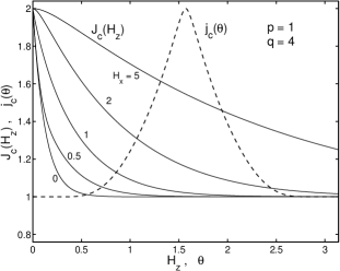
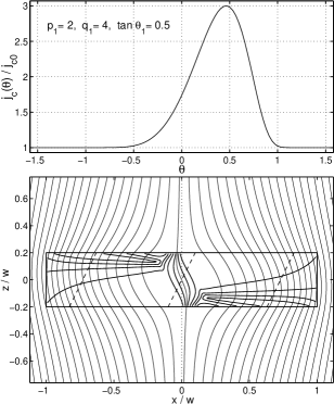
We now present an example of such calculations for this type of pinning. Let at $H_{ax}=0$ the following dependence $J_{c}(H_{z})$ be extracted from some experimental magneto-optics data:

$$J_{c}(H_{z})=j_{c}(0)d\left[1+p\,\exp\left(-{q\,H_{z}\over H_{cr}}\right)\right]\,,$$ (16)

where $H_{cr}=j_{c}(0)d/2$, while $j_{c}(0)$ and the dimensionless $p$ and $q$ are positive constants. Using Eqs. (C), one can easily verify that the corresponding angular dependence of the critical current density takes the form:

$$j_{c}(\theta)=j_{c}(0)\left[1+p\,(1+q\,t)\exp(-q\,t)\right]\,,$$

$$\tan\theta=t^{-1}\left[1+p\,\exp(-q\,t)\right]\,,$$ (17)

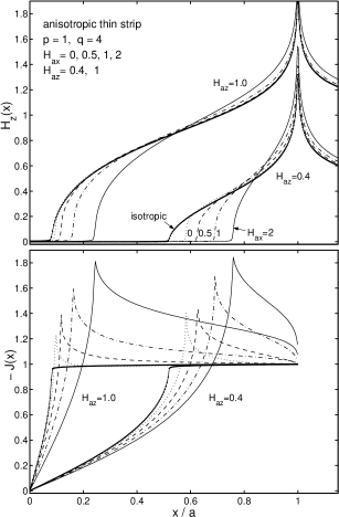
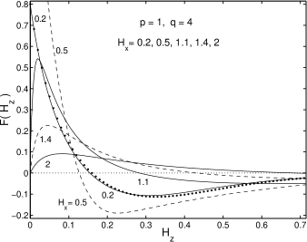
where $t$ is a curve parameter with range $0\leq t\leq\infty$. This dependence $j_{c}(\theta)$ is presented in Fig. 2 together with the function $J(H_{z})$, Eq. (16). Note that for $p>0$ the character of this dependence $j_{c}(\theta)$ is typical of layered high-$T_{c}$ superconductors, 1 i.e., $j_{c}$ is largest for $\theta=\pi/2$. The profiles $H_{z}(x)$ that correspond to this $J_{c}(H_{z})$ are shown in Fig. 3. In Figs. 2 and 3 we also show the dependences of $J_{c}$ on $H_{z}$ for $H_{ax}\neq 0$ and appropriate magnetic-field profiles in an oblique magnetic field. With the use of Eqs. (C), (14) - (16), we calculate the quantity $(\Delta H_{z}/d)(dH_{z}/dx)^{-1}$ as a function of $H_{z}$, Fig. 4. Interestingly, even at not too small $H_{ax}<0.4j_{c}(0)d$, formula (15) gives reasonable results. An example of the asymmetry of the $H_{z}$-profiles at the upper surface of the strip is presented in Fig. 1. This asymmetry is found from the data of Fig. 4, the known derivative $dH_{z}(x)/dx$, Fig. 3, and formulas of Appendix B (when $|x|<a$). Note that the steepness of $H_{z}(x)$ near $x=a$ has a pronounced effect on the form of $\Delta H_{z}(x)$ (and this steepness essentially depends 1 on the sign of $p$). The discontinuities of $\Delta H_{z}(x)$ at $x=\pm a$, $0$, $\pm w$ are caused by the inapplicability of our formulas for $\Delta H_{z}$ there. For comparison, we also show $\Delta H_{z}(x)$ and the profiles $H_{z}(x,0)$ and $H_{z}(x,d/2)$ calculated directly by solving the two-dimensional critical state problem for a strip of finite thickness.EH1 In this two-dimensional calculation the discontinuities of $\Delta H_{z}$ are smoothed out on scales of the order of $d$.

IV Strip with inclined defects in perpendicular magnetic field

In a recent Letter t the position of the so-called central d-line (the discontinuity line) at the upper surface of a thin rectangular YBa₂Cu₃O_7-δ platelet was measured by magneto-optical imaging. In this d-line the sheet current changes its sign and the magnetic field $H_{z}$ reaches an extremum (a minimum). When columnar defects tilted to the c-axis were introduced into the sample, the d-line shifted relative to the central axis of the platelet, t and the value of this shift first increased and then decreased with increasing perpendicular magnetic field. As mentioned in the Introduction, the authors of Ref. t, explained the shift by the in-plane magnetization originating from a zigzag structure of vortices, and the disappearance of the magnetization and of this shift by loss of their interlayer coherence. It is clear that the shift of the d-line reflects the asymmetry of the magnetic field profiles at the upper surface of the sample.

Figure 5: Top: The anisotropic critical current density $j_{c}(\theta)$, Eq. (18) with $p_{1}=2$, $q_{1}=4$, and $\tan\theta_{1}=0.5$, that models pinning by tilted columnar defects. Bottom: Two-dimensional computation EH1 (creep exponent $\sigma=50\gg 1$; London depth $\lambda=w/30=d/12$; $120\times 28$ grid points) of the critical state in a long strip with rectangular cross section of aspect ratio $d/2w=0.2$ and with anisotropic pinning described by the $j_{c}(\theta)$ of the upper plot, exposed to a perpendicular field $H_{az}=0.2j_{c0}d$. Shown are the magnetic field lines (thin lines) and some contour lines of the current density $j(x,z)/j_{c0}=$ -2.75, -2.25, -1.75, $\dots$, 2.75 (thick lines). The three inclined dashed lines indicate the direction $\theta_{1}$ of the columnar pins. Note that the distribution of $j_{c}$ across the thickness of the strip is asymmetric; $|j_{c}(x,z)|$ is maximum where the field lines are along the defects, and $j_{c}\approx j_{c0}$ is nearly constant where the deviation from this direction is large. The line $j_{c}(x,z)=0$ coincides with the central magnetic field line.

The zigzag structure of vortices occurs when the tilt angle $\Delta\theta$ of the local ${\bf H}$ to the direction of the columnar defects is less than the so-called trapping angle $\theta_{t}$. bl1 In this case a misalignment of the local ${\bf H}$ and the averaged direction of the kinked flux lines appears, and this misalignment is of the order of $\epsilon^{2}(H_{c1}/H)(\theta_{t}-\Delta\theta)$ where $H_{c1}$ is the lower critical field and $\epsilon$ is the anisotropy parameter of the superconductor. The misalignment generates an in-plane magnetization $M_{x}\sim\epsilon^{2}H_{c1}(\theta_{t}-\Delta\theta)$, and hence one may expect that $\Delta H_{z}\approx-(d/dx)\int_{-d/2}^{d/2}M_{x}dz$; see Eq. (7). Note that if $\epsilon\to 0$ (the interlayer coherence is lost), $\Delta H_{z}$ tends to zero. This is just the mechanism of the asymmetry discussed in Ref. t, , and in this consideration the asymmetry is due to the equilibrium part of the in-plane magnetization. However, in our approximation, when $H\gg H_{c1}$ and ${\bf B}=\mu_{0}{\bf H}$, we neglect the misalignment, the fields of the order of $H_{c1}$, and the equilibrium part of magnetization. In our approach we take into account only the nonequilibrium part of magnetization, which also generates an asymmetry. This asymmetry can occur even if $H_{c1}\to 0$.

In Sec. III we have considered the case when the angular dependence of $j_{c}$ is symmetric about the $z$ axis [$j_{c}(-\theta)=j_{c}(\theta)$], and the asymmetry of the $H_{z}$ profiles is caused by an inclined applied magnetic field. However, such asymmetry can also result from the “opposite” situation when the applied field is along the $z$ axis while pinning is not symmetric about this axis. It is this situation that occurs when columnar defects are introduced at an angle $\theta_{1}$ to the $z$ axis. In this case $j_{c}(\theta)$ in the interval $|\Delta\theta|\equiv|\theta-\theta_{1}|<\theta_{t}$ is larger than outside this interval. The enhancement of $j_{c}$ in this interval is caused by the zigzag structure of vortices when a part of their length is trapped by strong columnar defects, while outside the interval pinning by the columnar defects is ineffective. Since flux lines are curved in the critical state, this enhancement of $j_{c}$ leads to an asymmetry of the current-density distribution across the thickness of the strip, and thus to a nonzero $\Delta H_{z}$. We carry out the calculation of the asymmetry of the $H_{z}$ profiles at the upper surface of the strip and of the shift of the d-line for the following dependence $j_{c}(\theta)$:

$$j_{c}(\theta)=j_{c0}\left[1+p_{1}\exp[-q_{1}(\tan\theta-\tan\theta_{1})^{2}]\right]\,,$$ (18)

which models an increased flux-line pinning by columnar defects at angles $\theta$ near $\theta_{1}$, Fig. 5. Here $p_{1}$ and $q_{1}$ are some positive dimensionless parameters ($q_{1}\sim\theta_{t}^{-2}$), and $j_{c0}$ is the current density in a sample without columnar defects ($j_{c0}$ describes, e.g., pinning by point defects). Although formulas (7) and (11) are still valid for thin strips with such $j_{c}(\theta)$, these formulas fail near the d-line, and so we carry out calculations of $\Delta H_{z}$ here, using the numerical solution EH1 of the two-dimensional critical state problem for a strip of finite thickness. In Fig. 5 we show the current and magnetic-field distributions in the strip with pinning described by Eq. (18), while in Fig. 6 the $H_{z}$ profiles and the shift of the d-line are presented.

Figure 6: Top: Asymmetric profiles of the magnetic field component $H_{z}(x,z)$ in the plane $z=0.52d$ slightly above the surface of the strip of Fig. 5 with anisotropic pinning by tilted columnar defects. Shown are the cases $p_{1}=2$ (solid lines) and $p_{1}=32$ (dashed lines), with $q_{1}=4$, $\tan\theta=0.5$, at applied field values $H_{az}=0.02$, $0.1$, $0.2$, $0.3$, $\dots$. Field unit is $j_{c0}d$. The slightly curved, nearly vertical lines with dots are the locus of the minima of these $H_{z}$ profiles. Bottom: The position $x_{\rm min}$ of the minimum of the profiles $H_{z}(x,0.52d)$ plotted versus the applied field $H_{az}$ for $p_{1}=2$ $\dots$ 256.

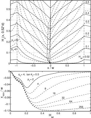
In Fig. 6 the decrease of the shift with increasing $H_{a}$ can be qualitatively explained as follows: The characteristic angle $\theta$ of the curved flux lines in the strip is of the order of $j_{c0}d/H_{z}$ [i.e., for most of the flux-line elements $\theta$ lies in the interval $-(j_{c0}d/H_{z})<\theta<(j_{c0}d/H_{z})$]. When the external magnetic field increases, this angle decreases and tends to zero. Thus, the flux-line pinning (the current distribution) becomes practically uniform across the thickness of the sample at sufficiently large $H_{az}$, and the shift vanishes. These considerations are valid for any type of anisotropic pinning, but there is one more reason for the disappearance of the shift in samples with columnar defects: When $\theta_{1}>\theta_{t}$ and $j_{c0}d/H_{z}$ is less than $\theta_{1}-\theta_{t}$, the zigzag structure of vortices disappears in the sample, and the flux-line pinning by these defects becomes ineffective. The trapping angle determining the width of the peak in $j_{c}$ decreases with increasing $H$ as some power of $H_{\Phi}/H$ if the applied field is of the order of the matching field $H_{\Phi}$ ($H_{\Phi}$ is a measure of the density of the columnar defects). bl1 Thus, if $\theta_{t}>\theta_{1}$ at $H=0$, the disappearance of the shift can occur at some magnetic field associated with $H_{\Phi}$. This is just observed in the experiment. t Note that in this case the disappearance of the shift is due to the disappearance of the zigzag structure of vortices in the superconductor rather than to the loss of the interlayer coherence.

Finally, we emphasize the unresolved problem of the analysis presented in this section: The shift calculated for the experimental ratio t $(d/w)\sim 0.06$ is noticeably less than the experimentally observed shift ($\Delta H_{z}$ decreases with decreasing $d$). A variation of the parameters $p_{1}$ and $q_{1}$ in Eq. (18) cannot change this conclusion. For example, although the maximum value of the function $|x_{\rm min}(H)|$ increases with $p_{1}$, it tends to a limit of the order of $(d/2)\tan\theta_{1}$ at $p_{1}\gg 1$; see Fig. 6.

V Conclusions

We have considered $H_{z}$ profiles at the upper surface of a thin strip whose thickness $d$ is much less than its width $2w$. To the leading order in $d/w$, these profiles are symmetric in $x$, $H_{z}(-x,d/2)=H_{z}(x,d/2)$. However, the analysis to the next order in this small parameter reveals the asymmetry of the profiles, $H_{z}(x,d/2)-H_{z}(-x,d/2)$, which coincides with $\Delta H_{z}(x)\equiv H_{z}(x,d/2)-H_{z}(x,-d/2)$, the difference of $H_{z}$ at the upper and lower surfaces of the strip. We calculate $\Delta H_{z}(x)$ and show that this $\Delta H_{z}$ differs from zero in an oblique magnetic field ${\bf H}_{a}=(H_{ax},0,H_{az})$ and depends on the scenario of switching on this field. For definiteness, we analyze in detail the so-called third scenario obl1 when $H_{ax}$ is switched on before $H_{az}$.

In the region $|x|<a$ where the flux-free core occurs [where the symmetric part of $H_{z}(x)$ is almost equal to zero], the asymmetry of the $H_{z}$ profiles exists even for the ${\bf H}$-independent $j_{c}$ (the Bean model) and is due to the asymmetric shape of the flux-free core in the oblique magnetic field. Outside this region ($|x|>a$) the asymmetry appears only if $j_{c}$ depends on the magnitude of the local magnetic induction or if there is an out-of-plane anisotropy of $j_{c}$. The asymmetry of the magnetic field profiles in oblique magnetic fields was observed in Ref. w, ; see also Fig. 3e in Ref. I, .

An asymmetry of the $H_{z}$ profiles also appears when the flux-line pinning is not symmetric about the normal to the strip plane (about the $z$ axis). This situation occurs when inclined columnar defects are introduced into the strip. In this context we have discussed the experimental data of Itaka et al. t It is shown that although these data can be qualitatively understood from our results, there is a quantitative disagreement between the experimental and theoretical results on the d-line shift.

Appendix A Formulas for $H_{z}$ at the surfaces of the strip

Using the Biot-Savart law, the $H_{z}$ component of the magnetic field at the point ($x_{0}$,$z_{0}$) of the strip can be written in the form:

$$H_{z}(x_{0},z_{0})=H_{az}\!+\!{1\over 2\pi}\!\int_{-d/2}^{d/2}\!\!\!\!\!\!dz\!\int_{-w}^{w}\!\!\!\!\!\!dx\,{j_{y}(x,z)(x\!-\!x_{0})\over r^{2}}\,.\$$ (19)

where $r^{2}=(x-x_{0})^{2}+(z-z_{0})^{2}$. Using the smallness of the ratio $d/w$, we now simplify this formula. Let us consider the integral

$$Q(z,x_{0},z_{0})=\!\!\int_{-w}^{w}\!\!\!\!\!\!dx\,j_{y}(x,z)\!\left[{(x-x_{0})\over r^{2}}-{1\over(x-x_{0})}\right]$$ (20)

which appears if one calculates the difference between the expression (19) and formula (4) for the infinitely thin strip. The main contribution to this $Q(z,x_{0},z_{0})$ is determined by the $x$ values near $x_{0}$, $|x-x_{0}|\sim d$. Since the current density $j_{y}(x,z)$ in the critical state of the strip changes in the $x$ direction on a scale which considerably exceeds $d$, in the calculation of $Q(z,x_{0},z_{0})$ we may use the expansion, $j_{y}(x,z)\approx j_{y}(x_{0},z)+(x-x_{0})j_{y}^{\prime}(x_{0},z)$ where $j_{y}^{\prime}(x_{0},z)\equiv\partial j_{y}(x_{0},z)/\partial x_{0}$. Inserting this expansion into integral (20), we find that

$$Q(z,x_{0},z_{0})\!\approx\!-\pi j_{y}^{\prime}(x_{0},z)|z\!-\!z_{0}|\!+\!j_{y}(x_{0},z){\rm O}({d^{2}\over w^{2}}),~{}~{}$$ (21)

and the last term in this expression may be omitted. Putting $z_{0}=\pm d/2$, we find

$${1\over 2\pi}\!\int_{-d/2}^{d/2}\!\!\!Q(z,x_{0},\pm{d\over 2})dz=-{dJ\over dx_{0}}{d\over 4}\pm{1\over 2}\Delta H_{z}(x_{0})\,,$$ (22)

where $\Delta H_{z}(x)$ is given by formula (7), and $J(x)$ is the sheet current,

$$J(x)\equiv\int_{-d/2}^{d/2}j_{y}(x,z)dz.$$

Eventually we arrive at

$$H_{z}^{\pm}(x)\!=\!H_{az}+\!{1\over 2\pi}\!\!\int_{-w}^{w}\!\!{J(t)\,dt\over t-x}-{dJ(x)\over dx}{d\over 4}\pm{\Delta H_{z}(x)\over 2}\,.$$ (23)

The first two terms in Eqs. (23) yield $H_{z}(x)$ for the infinitely thin strip, while the third and forth terms are corrections to this result due to the finite thickness of the strip. These corrections are relatively small (of the order of $d/w$).

The above derivation of Eq. (22) fails in the region of the strip, $|x|\leq a$, where a flux-free core occurs in the sample. The boundary of the core, $x_{f}(z)$ [or equivalently $z_{f}(x)$], can be calculated from $J(x)$ at $|x|<a$; see Ref. 1, . In this region, the flux lines are practically parallel to the surfaces of the sample, and they are sandwiched between the surfaces and the core. If $|x_{0}-x_{f}(z_{0})|\lesssim d$, i.e., if the point ($x_{0}$, $z_{0}$) lies near the boundary of the flux-free core, one cannot transform Eq. (20) into Eq. (21). However, at $|x|<a$ we can repeat the above analysis, integrating over $z$ rather than over $x$ in expression (20). If $j_{y}(x,z)$ is almost independent of $z$ in the region between the core and the surfaces of the sample, we eventually arrive at the same formula (22) for $|x|<a$. This formula fails only in the vicinity of the points $x=\pm a$ which are the positions of the flux front for the infinitely thin strip and near the points $x=0$, $x=\pm w$.

Figure 7: The current and flux fronts in a thin strip to which first the in-plane magnetic field component $H_{ax}$ is applied and then the perpendicular $H_{az}$ (scenario 3). Shown are the fronts for $H_{ax}=0$, 0.15, 0.35, 0.45 and 0.5 (or larger), and $H_{az}=0.25$ in units of $j_{c}d$. The fronts for other values of $H_{az}$ are scaled with $a$. The lines $z_{\gamma}^{+}(x)$, $z_{\gamma}^{-}(x)$, $z_{1}(x)$, $z_{2}(x)$ are described in Appendix B.

Appendix B Flux-free core for the third scenario

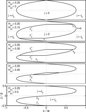
In Ref. mbi, for a thin strip in an oblique magnetic field, the shapes of the flux-free core and of the lines separating regions with opposite directions of the critical currents were presented only for two scenarios of switching on the external magnetic field (1: at constant angle $\theta_{0}$, 2: first $H_{az}$ then $H_{ax}$). Below we present the corresponding formulas for the third scenario (when $H_{ax}$ is applied before $H_{az}$). As in Ref. mbi, , we shall use the Bean model here, i.e., we assume that $j_{c}$ is constant. However, the formulas of this Appendix remain true also for the case $j_{c}=j_{c}(\theta)$ where $\theta$ is the angle between the local direction of ${\bf H}$ and the $z$ axis; see below.

Let $x=\pm a$ be the positions of the flux front in the infinitely thin strip. Within the Bean model, the sheet current $J(x)$ at $-a\leq x\leq a=w/{\rm cosh}(\pi H_{az}/j_{c}d)$ is B1 ; B2

$$J(x)=-{2\over\pi}J_{c}\,{\rm arctan}{x\sqrt{w^{2}-a^{2}}\over\sqrt{a^{2}-x^{2}}}\,.$$ (24)

In Fig. 7 we show the lines $z_{1}(x)$ and $z_{2}(x)$ separating the regions with opposite directions of the critical currents and the flux-free core composed of the lines $z_{\gamma}^{+}(x)$ and $z_{\gamma}^{-}(x)$. Using the method of Ref. mbi, , we find the formulas that describe $z_{1}(x)$, $z_{2}(x)$, $z_{\gamma}^{+}(x)$ and $z_{\gamma}^{-}(x)$ at $-a\leq x\leq 0$. The appropriate formulas for $a\geq x\geq 0$ can be obtained by the substitution: $x\to-x$, $z\to-z$.

When $H_{ax}\leq j_{c}d/4$ and $-x_{1}\leq x\leq 0$, one has

$$z_{\gamma}^{+}(x)={d\over 2}-{H_{ax}\over j_{c}}-{J(x)\over 2j_{c}},$$ (25)

$$z_{\gamma}^{-}(x)={H_{ax}\over j_{c}}-{d\over 2},$$ (26)

$$z_{1}(x)={J(x)\over 4j_{c}}-{d\over 2},$$ (27)

while if $-a\leq x\leq-x_{1}$, the $z_{\gamma}^{+}(x)$ is still given by Eq. (25), but

$$z_{\gamma}^{-}(x)={J(x)\over 2j_{c}}-{H_{ax}\over j_{c}}-{d\over 2}.$$ (28)

Here $J(x)$ is the sheet current at the point $x$, and the point $x_{1}$ follows from the condition $|J(x_{1})|=4H_{ax}$.

When $j_{c}d/4\leq H_{ax}\leq j_{c}d/2$ and $-x_{2}\leq x\leq 0$, the functions $z_{\gamma}^{+}(x)$, $z_{\gamma}^{-}(x)$, $z_{1}(x)$ are described by formulas (25)-(27) where the point $x_{2}$ is determined by the condition $|J(x_{2})|=2j_{c}d-4H_{ax}$. At $-a\leq x\leq-x_{2}$ only the lines $z_{1}(x)$, $z_{2}(x)$ exist; the line $z_{1}(x)$ is given by Eq. (27), while

$$z_{2}(x)=-{J(x)\over 4j_{c}}.$$ (29)

For high values of $H_{ax}$, when $j_{c}d/2\leq H_{ax}$, the flux-free core disappears, and one has Eq. (27) for $z_{1}(x)$ and Eq. (29) for $z_{2}(x)$ at $-a\leq x\leq 0$.

Using the formulas of this Appendix and Eq. (5), it is easy to calculate $\Delta H_{z}(x)$ in the region $|x|\leq a$. One has

$$\Delta H_{z}(-a\leq x\leq x_{1})=-{H_{ax}\over j_{c}}{dJ\over dx},$$ (30)

$$\Delta H_{z}(-x_{1}\leq x\leq 0)=-{0.25J+H_{ax}\over 2j_{c}}{dJ\over dx},$$ (31)

at $H_{ax}\leq j_{c}d/4$,

$$\Delta H_{z}(-a\leq x\leq x_{2})=-{d\over 4}\left({dJ\over dx}\right),$$ (32)

$$\Delta H_{z}(-x_{2}\leq x\leq 0)=-{0.25J+H_{ax}\over 2j_{c}}{dJ\over dx},$$ (33)

at $j_{c}d/4\leq H_{ax}\leq j_{c}d/2$, and Eq. (B9) at $j_{c}d/2\leq H_{ax}$ in the whole interval $-a\leq x\leq 0$. When $0\leq x\leq a$, one can use $\Delta H_{z}(x)=-\Delta H_{z}(-x)$.

The formulas of this Appendix are applicable to the case $j_{c}=j_{c}(\theta)$ since at $|x|\leq a$, the flux lines are practically parallel to the strip plane and $\theta\approx\pi/2$. Hence, it is sufficient to put $j_{c}=j_{c}(\pi/2)$ in the above formulas and to use $J(x)$ obtained numerically from the appropriate solution of the critical state problem for the infinitely thin anisotropic strip.

Appendix C $j_{c}(\theta)$ and $J_{c}(H_{z},H_{ax})$ in terms of $J_{c}(H_{z},0)$

When $j_{c}$ depends only on $\theta$, one can reconstruct this dependence from the $J_{c}(H_{z})$ obtained at $H_{ax}=0$: 1 ; obl1

$$j_{c}(\theta)d=J_{c}(H_{z})-H_{z}{dJ_{c}(H_{z})\over dH_{z}}\,,$$

$$\tan\theta={J_{c}(H_{z})\over 2H_{z}}\,.$$ (34)

Inserting this parametric form of $j_{c}(\theta)$ into Eq. (2), we arrive at equations determining $J_{c}(H_{z})$ at $H_{ax}\neq 0$, obl1

$${0.5J_{c}(H_{z},H_{ax})+H_{ax}\over H_{z}} = {J_{c}(t_{+},0)\over 2t_{+}},$$

$${|0.5J_{c}(H_{z},H_{ax})-H_{ax}|\over H_{z}} = {J_{c}(t_{-},0)\over 2t_{-}},$$

$${1\over H_{z}} = {1\over 2t_{+}}+\sigma{1\over 2t_{-}},$$ (35)

where $\sigma$ is the sign of $[0.5J_{c}(H_{z},H_{ax})-H_{ax}]$, $J_{c}(H_{z},H_{ax})$ denotes $J_{c}(H_{z})$ at a given value of $H_{ax}$, and hence $J_{c}(t,0)$ is the sheet current at $H_{ax}=0$. At $H_{ax}=0$ one has $t_{+}=t_{-}=H_{z}$, and Eqs. (C) reduce to $J_{c}=J_{c}(H_{z},0)$ as it should be. From the three Eqs. (C) for the three unknown variables $J_{c}$, $t_{+}$, $t_{-}$ ($t_{+}$ and $t_{-}$ are auxiliary variables) one finds $J_{c}(H_{z})$ at $H_{ax}\neq 0$. The magnetic field profiles in oblique applied field are then obtained by inserting this effective law $J_{c}(H_{z})$ into the critical state equations for the infinitely thin strip, Eqs. (4) - (6).

References

- (1) K. Itaka, T. Shibauchi, M. Yasugaki, T. Tamegai, S. Okayasu, Phys. Rev. Lett. 86, 5144 (2001).
- (2) G. D. Gheorghe, M. Menghini, R. J. Wijngaarden, (unpublished).
- (3) G. P. Mikitik and E. H. Brandt, Phys. Rev. B62, 6800 (2000).
- (4) E. H. Brandt and G. P. Mikitik, Phys. Rev. B. (to be published).
- (5) E. H. Brandt, Phys. Rev. B49, 9024 (1994).
- (6) E. H. Brandt, Phys. Rev. B64, 024505 (2001); ibid 54, 4246 (1996).
- (7) The idea of the imbalance of the currents (see Fig. 4c in Ref. t, ) leads to “opposite” current distributions for the upper and lower surfaces of the sample. Since the currents flowing on both these surfaces almost equally generate , the asymmetry of the profiles was considerably overestimated in Ref. t, .
- (8) G. P. Mikitik, E. H. Brandt, and M. Indenbom, Phys. Rev. B70, 014520 (2004).
- (9) M. V. Indenbom, Th. Shuster, M. R. Koblischka, A. Forkl, H. Kronmüller, L. A. Dorosinskii, V. K. Vlasko-Vlasov, A. A. Polyanskii, R. L. Prozorov, V. I. Nikitenko, Physica C 209, 259 (1993).
- (10) M. R. Koblischka, R. J. Wijngaarden, Supercond. Sci. Technol. 8, 189 (1995).
- (11) Ch. Jooss, J. Albrecht, H. Kuhn, S. Leonhardt, and H. Kronmüller, Rep. Prog. Phys. 65, 651 (2002).
- (12) F. Laviano, D. Botta, A. Chiodoni, R. Gerbaldo, G. Ghigo, L. Gozzelino, and E. Mezzetti, Phys. Rev. B68, 014507 (2003).
- (13) E. Zeldov, D. Majer, M. Konczykowski, A. I. Larkin, V. M. Vinokur, V. B. Geshkenbein, N. Chikumoto, and H. Shtrikman, Europhys. Lett. 30, 367 (1995).
- (14) B. J. Roth, N. G. Sepulveda, J. P. Wikswo,Jr, J. Appl. Phys. 65, 361 (1989).
- (15) E. H. Brandt, Phys. Rev. B46, 8628 (1992).
- (16) P. D. Grant, M. V. Denhoff, W. Xing, P. Brown, S. Govorkov, J. C. Irwin, B. Heinrich, H. Zhou, A. A. Fife, A. R. Cragg, Physica C 229, 289 (1994).
- (17) R. J. Wijngaarden, H. J. W. Spoelder, R. Surdeanu, R. Griessen, Phys. Rev. B54, 6742 (1996).
- (18) T. H. Johansen, M. Baziljevich, H. Bratsberg, Y. Galperin, P. E. Lindelof, Y. Shen, P. Vase, Phys. Rev. B54, 16264 (1996).
- (19) A. E. Pashitski, A. Gurevich, A. A. Polyanskii, D. S. Larbalestier, A. Goyal, E. D. Specht, D. M. Kroeger, J. A. DeLuca, J. E. Tkaczyk, Science 275, 367 (1997).
- (20) Ch. Jooss, R. Warthmann, A. Forkl, H. Kronmüller, Physica C 299, 215 (1998).
- (21) G. Blatter, M. V. Feigel’man, V. B. Geshkenbein, A. I. Larkin, V. M. Vinokur, Rev. Mod. Phys. 66, 1125 (1994).
- (22) See Secs. IX A1 and IX B5 in Ref. bl, .
- (23) M. V. Indenbom, C. J. van der Beek, M. Konczykowski, F. Holtzberg, Phys. Rev. Lett. 84, 1792 (2000).
- (24) E. H. Brandt and M. V. Indenbom, Phys. Rev. B48, 12893 (1993).
- (25) E. Zeldov, J. R. Clem, M. McElfresh, and M. Darwin, Phys. Rev. Bbf 49, 9802 (1994).