A Mutual Selection Model for Weighted Networks

Abstract

For most networks, the connection between two nodes is the result of their mutual affinity and attachment. In this paper, we propose a mutual selection model to characterize the weighted networks. By introducing a general mechanism of mutual selection, the model can produce power-law distributions of degree, weight and strength, as confirmed in many real networks. Moreover, we also obtained the nontrivial clustering coefficient $C$, degree assortativity coefficient $r$ and degree-strength correlation, depending on a model parameter $m$. These results are supported by present empirical evidences. Studying the degree-dependent average clustering coefficient $C(k)$ and the degree-dependent average nearest neighbors’ degree $k_{nn}(k)$ also provide us with a better description of the hierarchies and organizational architecture of weighted networks.

I Introduction

In the past few years, there has been a great devotion of physicists to understand and characterize the underlying mechanisms of complex networks, e.g. the Internet Internet , the WWW WWW , the scientific collaboration networks (SCN) CN1 ; CN2 ; CN3 and world-wide airport networks (WAN)air1 ; air2 ; air3 . Until now, network researchers have mainly focused on the topological aspect of graphs, that is, unweighted networks. Typically, Barabási and Albert proposed a famous model (BA model) that introduces the linear degree preferential attachment mechanism to study unweighted growing networks BA . In their model, however, if one considers other measures like the clustering coefficient then one may conclude that this model is still insufficient to describe reality. The hypothesis of a linear attachment rate is empirically supported by measuring different real networks, but the origin of the ubiquity of the linear preferential attachment is not clear yet. Most recently, the availability of more complete empirical data has allowed scientists to consider the variation of the weights of links that reflect the physical characteristics of many real networks. It is well-known that networks are not only specified by their topology but also by the dynamics of weight taking place along the links. For instance, the heterogeneity in the intensity of connections may be very important in understanding network systems. The amount of traffic characterizing the connections of communication systems or large transport infrastructure is fundamental for a full description of these networks. Take the WAN for example: each given edge weight $w_{ij}$ (traffic) is the number of available seats on direct flight connections between the airports $i$ and $j$. In the SCN, the nodes are identified with authors and the weight depends on the number of coauthored papers. Obviously, there is a tendency for a modelling approach to networks that goes beyond the purely topological point of view. In the light of this need, Alain Barrat, et al. presented a model (BBV model) that integrates the topology and weight dynamical evolution to study the growth of weighted networks BBV . Their model yields scale-free properties of the degree, weight and strength distributions, controlled by an introduced parameter $\delta$. However, its weight dynamical evolution is triggered only by newly added vertices, hardly resulting in satisfying interpretations to the collaboration networks or the airport systems.

The properties of a graph can be expressed via its adjacency matrix $a_{ij}$, whose elements take the value 1 if an edge connects the vertex $i$ to the vertex $j$ and 0 otherwise. The data contained in the previous data sets permit to go beyond this topological representation by defining a weighted graph. Weighted networks are often described by a weighted adjacency matrix $w_{ij}$ which represents the weight on the edge connecting vertices $i$ and $j$, with $i,j=1,\ldots,N$, where $N$ is the size of the network. We will only consider undirected graphs, where the weights are symmetric ($w_{ij}=w_{ji}$). As confirmed by measurements, complex networks often exhibit a scale-free degree distribution $P(k)\thicksim k^{-\gamma}$ with 2$\leq\gamma\leq$3 air1 ; air2 . The weight distribution $P(w)$ that any given edge has weight $w$ is another significant characterization of weighted networks, and it is found to be heavy tailed, spanning several orders of magnitude ref1 . A natural generalization of connectivity in the case of weighted networks is the vertex strength described as $s_{i}=\sum_{j\in\Gamma(i)}w_{ij}$, where the sum runs over the set $\Gamma(i)$ of neighbors of node $i$. The strength of a vertex integrates the information about its connectivity and the weights of its links. For instance, the strength in WAN provides the actual traffic going through a vertex and is obvious measure of the size and importance of each airport. For the SCN, the strength is a measure of scientific productivity since it is equal to the total number of publications of any given scientist. This quantity is a natural measure of the importance or centrality of a vertex in the network. Empirical evidence indicates that in most cases the strength distribution has a fat tail air2 , similar to the power law of degree distribution. Highly correlated with the degree, the strength usually displays scale-free property $s\thicksim k^{\beta}$ traffic-driven ; empirical ; empirical2 ; hierarchy .

The previous models of complex networks always incorporate the (degree or strength) preferential attachment mechanism, which may result in scale-free properties. Essentially speaking, this mechanism just describes interactions between the newly-added node and the old ones. The fact is that such interactions also exist between old nodes. This perspective has been practised in the work of Dorogovtsev and Mendes (DM) DM who proposed a class of undirected and unweighted models where new edges are added between old sites (internal edges) and existing edges can be removed (edge removal). On the other hand, we argue that any connection is a result of mutual affinity and attachment between nodes, while many network models seem to ignore this point. Traditional models often present us such an evolution picture: pre-existing nodes are passively attached by newly adding nodes according to linear degree (or strength) preferential mechanism. This picture is just a partial aspect for most complex networks. It is worth remarking that the creation and reinforcement of internal connections are an important aspect for understanding real graphs.

In this paper, we shall present a model for weighted networks that considers the topological evolution under the general mechanism of mutual selection and attachment between vertices. It can mimic the reinforcement of internal connections and the evolution of many infrastructure networks. The diversity of scale-free characteristics, nontrivial clustering coefficient, assortativity coefficient and nonlinear strength-degree correlation that have been empirically observed can be well explained by our microscopic mechanisms. Moreover, in contrast with previous models where weights are assigned statically ref2 ; ref3 or rearranged locally BBV , we allow weights to be widely updated.

II The Mutual Selection Model

The model starts from an initial configuration of $N_{0}$ vertices fully connected by links with assigned weight $w_{0}$. The model is defined on two coupled mechanisms: the topological growth and the mutual selection dynamics:

(i)Topological Growth. At each time step, a new vertex is added with $n$ edges connected to $n$ previously existing vertices, choosing preferentially nodes with large strength; i.e. a node $i$ is chosen according to the strength preferential probability:

$$\Pi_{new\rightarrow i}=\frac{s_{i}}{\sum_{k}s_{k}}.$$ (1)

The weight of each new edge is also fixed to $w_{0}$.

(ii)Mutual Selection Dynamics. Every existing node $i$ selects $m$ other pre-existing nodes for possible connection according to the probability:

$$\Pi_{i\rightarrow j}=\frac{s_{j}}{\sum_{k}s_{k}-s_{i}}.$$ (2)

Considering the normalization requirement and that vertices are not permitted to connect themselves, the denominator of $\Pi_{i\rightarrow j}$ contains the term $-s_{i}$. If two unconnected nodes are mutually selected, then an internal connection is built between them. If two connected nodes are mutually selected, then their connection is strengthened; i.e. their edge weight is increased by $w_{0}$. Here the parameter $m$ is the number of candidate vertexes for creating or strengthening connections. Later, we will see that $m$ also controls the growing speed of the network’s total strength; for instance, the increasing rate of total information in a communication system.

We argue that connections in most real networks are due to the mutual selections and attachments between nodes. Take the SCN for example: the collaborations among scientists require their common interest and mutual acknowledgements. Unilateral effort does not promise collaboration. Two scientists that both have strong scientific potentials (large strengths) and long collaborating history are more likely to publish papers together during a certain period. Likewise, for the Movie Actor Collaboration Networks (MACN), two actors that both have high popularity, if they co-star, are more probably to boost up the box office. So it is reasonable to assume that each node is more likely to choose those nodes with large strengths when building or strengthening connections. But pre-existing nodes with large strengths will not be passively attached by nodes with small strength. There are competition and adaptation in such a complex systems. Both natural and social networks bear such a property or mechanism during their evolutions. The above description of our model could satisfactorily explain the WAN too. The weight here denotes the relative magnitude of the traffic on a flight connection. At the beginning of the construction of the airport network, the air traffic is usually open between metropolises that hold a high status in both economy and politics. Once a new airline is created between two airports, it will trigger a more intense traffic activity depending on the specific nature of the network topology and on the micro dynamics. With the improvement of national economy and the expansion of population, the air traffic between metropolises will increase. Due to their importance, there is an obvious need for other cities to build new airports to connect the metropolises. Yet, it is reasonable that the traffic between metropolises will grow faster than that between other cities, each of which holds a lower economical and political status and a smaller population that can afford airplanes. But due to the limit of energy and resources, each node can only afford a limited number of connections. Hence facing the vertex pool, they have to choose. For instance, in the WAN, an airport can not afford the cost of connecting all the other airports.

The network provides the substrate on which numerous dynamical processes occur. Technology networks provide large empirical database that simultaneously captures the topology and the dynamics taking place on it. For Internet, the information flow between routers (nodes) can be represented by the corresponding edge weight. The total information load that each router deals with can be denoted by the node strength, which also represents the importance of given router. The increasing information flow as an internal demand always spurs the expansion of technological networks. Specifically, the largest contribution to the growth is given by the emergence of links between already existing nodes. This clearly points out that the Internet growth is strongly driven by the need of a redundancy wiring and an increasing need of available bandwidth for data transmission empirical . On one end, newly-built links (between existing routers) are supposed to preferentially connect high strength routers, because otherwise, it would lead to the unnecessary traffic congestion along indirect paths that connect those high strength nodes. Naturally, information traffic along existing links between high strength routers, in general, increases faster than that between low strength routers. This phenomenon could be reproduced in our model too. On the other end, new routers preferentially connect to routers with larger bandwidth and traffic handling capabilities (the strength driven attachment). This characteristic also exists in airport system, power grid, and railroad network; and they could be explained by our mechanisms.

III Probability Distributions and Strength Evolution

The network growth starts from an initial seed of $N_{0}$ nodes, and continues with the addition of one node per unit time, until a size $N$ is reached. Hence the model time is measured with respect to the number of nodes added to the graph, i.e. $t=N-N_{0}$, and the natural time scale of the model dynamics is the network size $N$. Using the continuous approximation, we can treat $k$, $w$, $s$ and the time $t$ as continuous variables Internet ; BA . Then the edge weight $w_{ij}$ is updated as this evolution equation:

$$\frac{dw_{ij}}{dt} = m\frac{s_{j}}{\sum_{k}s_{k}-s_{i}}\times m\frac{s_{i}}{\sum_{k}s_{k}-s_{j}}$$ (3)

$$= \frac{m^{2}s_{i}s_{j}}{(\sum_{k}s_{k}-s_{j})(\sum_{k}s_{k}-s_{i})}.$$

There are two processes that contribute to the increment of strength $s_{i}$. One is the creation or reinforcement of internal connections incident with node $i$, the other is the attachment to $i$ by newly added node. So the rate equation of strength $i$ can be written as below:

$$\frac{ds_{i}}{dt} = \sum_{j}\frac{dw_{ij}}{dt}+n\times\frac{s_{i}}{\sum_{k}s_{k}}$$ (4)

$$\approx \frac{m^{2}s_{i}}{\sum_{k}s_{k}}\frac{\sum_{j}s_{j}}{\sum_{k}s_{k}}+\frac{ns_{i}}{\sum_{k}s_{k}}$$

$$= (m^{2}+n)\frac{s_{i}}{\sum_{k}s_{k}}.$$

This equation may be written in a more compact form by noticing that

$$\sum_{i=1}^{t}s_{i}=\int_{0}^{t}\sum_{k\in\Lambda}\frac{ds_{k}}{dt}dt+nt\approx(m^{2}+2n)t,$$ (5)

where $\Lambda$ represents the set of existing nodes at time step $t$. By plugging this result into the equation (4), we obtain the following strength dynamical equation

$$\frac{ds_{i}}{dt}=\frac{m^{2}+n}{m^{2}+2n}\frac{s_{i}}{t},$$ (6)

which can be readily integrated with initial conditions $s_{i}(t=i)=n$, yielding

$$s_{i}(t)=n(\frac{t}{i})^{\frac{m^{2}+n}{m^{2}+2n}}.$$ (7)

The equation $\sum_{i}s_{i}\approx(m^{2}+2n)t$ also indicates that the total strength of the vertices in statistical sense is uniformly increased with the size of network. As one see, the growing speed of the network’s total strength load is mainly determined by the model parameter $m$.

The knowledge of the time-evolution of the various quantities allows us to compute their statistical properties. Indeed, the time $t_{i}=t$ at which the node $i$ enters the network is uniformly distributed in [0,t] and the degree probability distribution can be written as

$$P(s,t)=\frac{1}{t+N_{0}}\int_{0}^{t}\delta(s-s_{i}(t))dt_{i},$$ (8)

where $\delta(x)$ is the Dirac delta function. Using equation $s_{i}(t)\sim(t/i)^{\theta})$ obtained from Eq. (7), one obtains in the infinite size limit $t\rightarrow\infty$ the distribution $P(s)\sim s^{\alpha}$ with $\alpha=1+1/\theta$:

$$\alpha=2+n/(m^{2}+n).$$ (9)

Obviously, when $m=0$ the model is topologically equivalent to the BA network and the value $\alpha=3$ is recovered. For larger values of $m$, the distribution is gradually broader with $\alpha\rightarrow 2$ when $m\rightarrow\infty$.

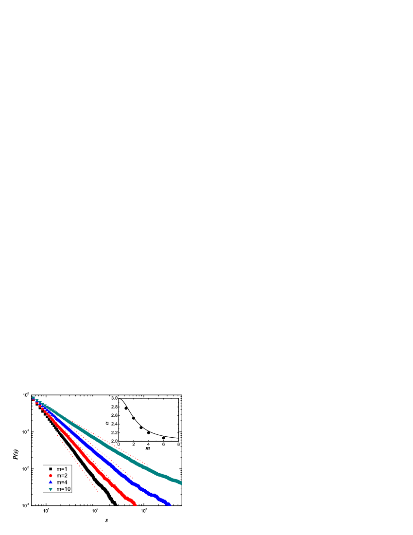
Figure 1: Probability distribution $P(s)$. Data are consistent with a power-law behavior $s^{-\alpha}$. In the inset we give the value of $\alpha$ obtained by data fitting (filled circles), together with the analytical expression $\alpha=2+n/(m^{2}+n)=2+5/(m^{2}+5)$(line). The data are averaged over 10 independent runs of network size N=5000.

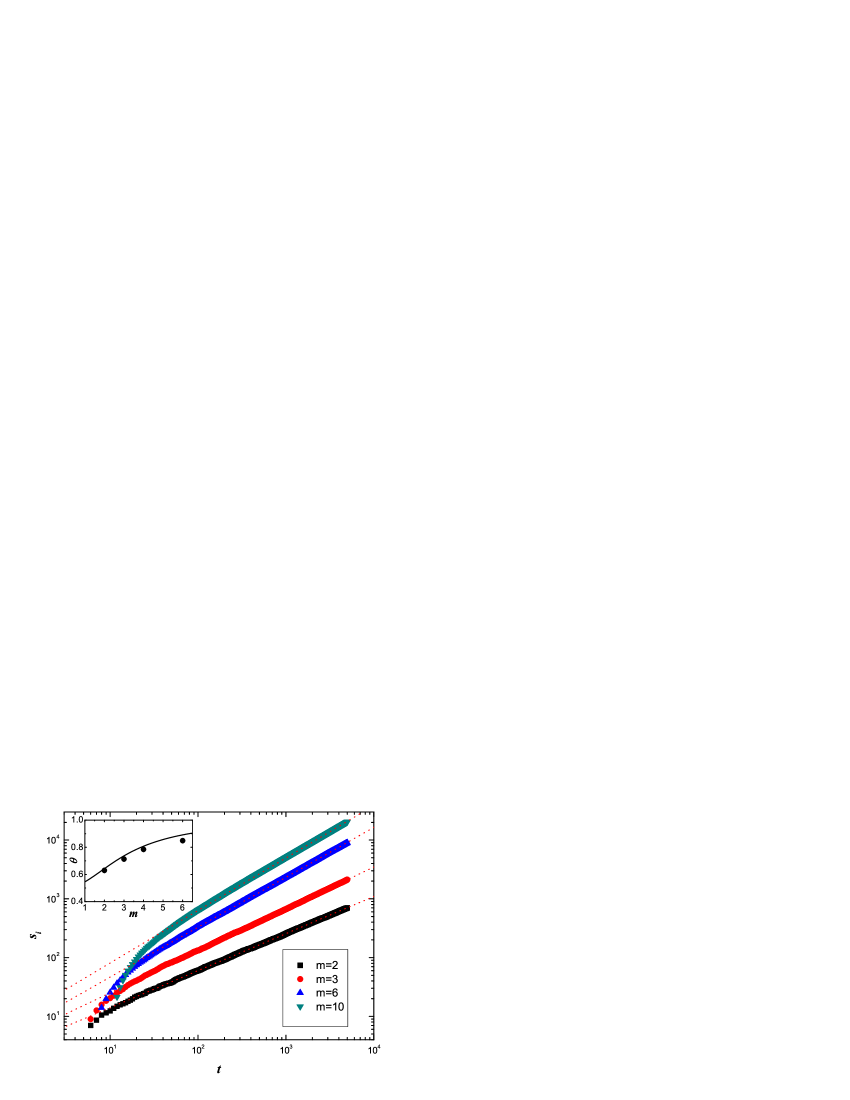
Figure 2: Evolution of strength of vertices during the growth of network for various of $m$. In the inset we give the value of $\theta$ obtained by data fitting (filled circles), together with the analytical expression $\theta=\frac{m^{2}+n}{m^{2}+2n}=\frac{m^{2}+5}{m^{2}+10}$(line).

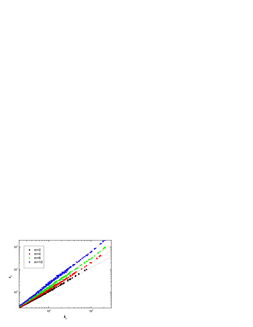
Figure 3: Strength $s_{i}$ versus $k_{i}$ for different $m$ (log-log scale). Linear data fitting gives slope 1.04, 1.16, 1.26 and 1.41 (from bottom to top), demonstrating the correlation of $s\sim k^{\beta}$.

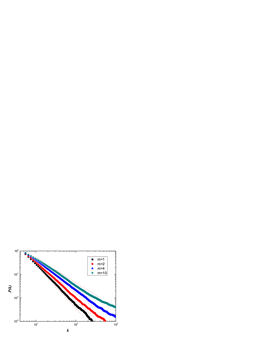
Figure 4: Probability distribution of the degrees $P(k)\sim k^{-\gamma}$ for different $m$. The data are averaged over 10 independent runs of network size N=5000.

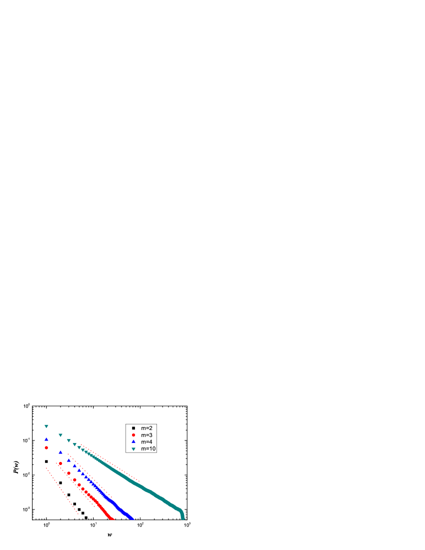
Figure 5: Probability distribution of the weights $P(w)\sim w^{-\eta}$ for various $m$. The data are averaged over 10 independent runs of network size N=5000.

We performed numerical simulations of networks generated by choosing different values of $m$ and fixing $n=5$ and $w_{0}=1$. Considering that every vertex strength can at most increase by $m$ from internal connections and a newly added node can at most connect with $n$ existing nodes, it is easy to see that the initial network configuration must satisfy $N_{0}=\max(m+1,n)$. So for example, if $m=10$, then $N_{0}=11$. We have checked that the scale-free properties of our model networks are independent of the initial conditions. Numerical simulations are consistent with our theoretical predictions, verifying again the reliability of our present results. Fig. 1 gives the probability distribution $P(s)\sim s^{\alpha}$, which is in excellent agreement with the theoretical predictions. In Fig. 2 we show the behavior of the vertices’ strength versus time for different values of $m$, recovering the behavior predicted by analytical methods. We also report the average strength $s_{i}$ of vertices with degree $k_{i}$, which displays a nontrivial power-law behavior $s\sim k^{\beta}$ as confirmed by empirical measurement. Unlike BBV networks (where $\beta=1$), the exponent $\beta$ here varies with the parameter $m$ in a nontrivial way as shown in Fig. 3. The nontrivial $s\sim k^{\beta}$ correlation demonstrates the significant part of weight increment along existing edges. More importantly, one could check the scale-free property of degree distribution ($P(k)\sim k^{-\gamma}$) by combining $s\sim k^{\beta}$ with $P(s)\sim s^{-\alpha}$. Considering the conservation of probability

$$\int_{0}^{\infty}P(k)dk=\int_{0}^{\infty}P(s)ds,$$ (10)

we can readily calculate the exponent $\gamma$:

$$P(k)=P(s)\frac{ds}{dk}=s^{-\alpha}\beta k^{\beta-1}=\beta k^{-(\beta(\alpha-1)+1)},$$ (11)

giving $\gamma=\beta(\alpha-1)+1$. The scale-free properties of degree and weight obtained from simulations are presented in Fig. 4 and Fig. 5, respectively. The simulation consistence of scale-free properties indicates that our model can indeed produce power-law distributions of degree, weight and strength. In this case, the numerical simulations of the model reproduce the behaviors predicted by the analytical calculations.

IV Clustering and Correlation

Many real networks in nature and society share two generic properties: they are scale-free and they display a high degree of clustering. Along with the general vertices hierarchy imposed by the scale-free strength distribution, complex networks show an architecture imposed by the structural and administrative organization of these systems, which is mathematically encoded in the various correlations existing among the properties of different vertices. For this reason, a set of topological and weighed quantities are customarily studied in order to uncover the network architecture. A first and widely used quantity is given by the clustering of vertices. The clustering of a vertex $i$ is defined as

$$c_{i}=\frac{1}{k_{i}(k_{i}-1)}\sum_{j,h}a_{ij}a_{ih}a_{jh},$$ (12)

and measures the local cohesiveness of the network in the neighborhood of the vertex. Indeed, it yields the fraction of inter-connected neighbors of a given vertex. The average over all vertices gives the network clustering coefficient which describes the statistics of the density of connected triples. Further information can be gathered by inspecting the average clustering coefficient $C(j)$ restricted to classes of vertices with degree $k$:

$$C(k)=\frac{1}{NP(k)}\sum_{i,k_{i}=k}c_{i}.$$ (13)

In many networks, the average clustering coefficient $C(k)$ exhibits a highly nontrivial behavior with a power-law decay as a function of $k$hierarchy , indicating that low-degree nodes generally belong to well interconnected communities (high clustering coefficient) while high-degree sites are linked to many nodes that may belong to different groups which are not directly connected (small clustering coefficient). This is generally the signature of a nontrivial architecture in which hubs (high degree vertices) play a distinct role in the network. Numerical simulations indicate that for large $m$, the clustering coefficient $C(N)$ is almost independent of $N$ (as we can see in Fig. 6), which agrees with the finding in several real networks BA . Generally, when the network size $N$ is larger than 5000, the clustering coefficient is nearly stable. So most computer runs are assigned with 5000. Still, it is worth remarking that for the BA networks, $C(N)$ is nearly zero, far from the practical nets that exhibit a variety of small-world properties. In the present model, however, clustering coefficient $C$ is fortunately found to be a function of $m$ (see Fig. 7), also supported by empirical data in a broad range. Finally, the clustering coefficient $C(k)$ depending on connectivity $k$ for increasing $m$ is also interesting and shown in Fig. 8. For clarity, we add the dashed line with slope $-1$ in the log-log scale. This simulation results are supported by recent empirical measurements in many real networks. For the convenience of comparison with Fig. 8, we use two figures from Ref. [17] as our Fig. 9, from which one can see the agreements of theory and experiment are quite excellent. Empirical evidence generally supports the simulations of clustering-degree correlation. Though some previous modelsmm1 ; mm2 ; mm3 can generate the power-law decay of the clustering-degree correlation, none of them as far as we know can produce the flat head as found in real graphs. This is a special property that our model successfully behaves.

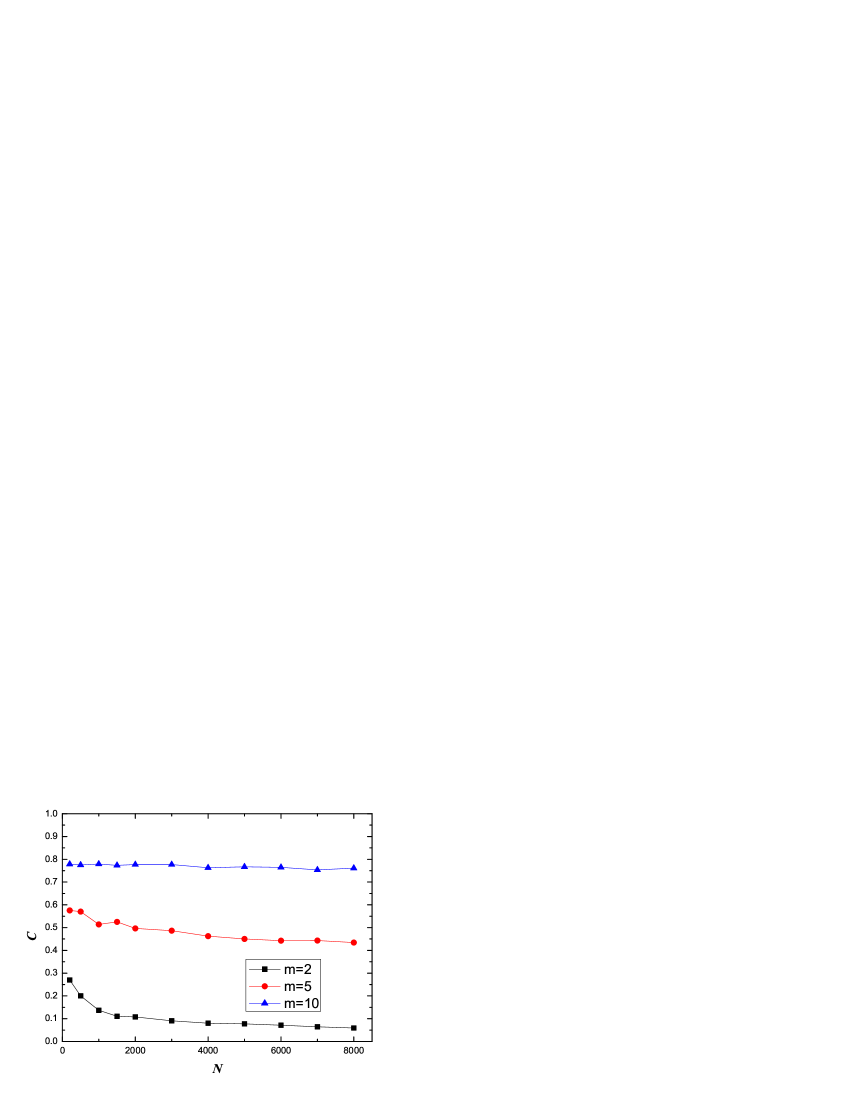
Figure 6: The evolution of clustering coefficient (or $C$ versus $N$) which converges soon.

Figure 7: Clustering coefficient $C$ depending on the parameter $m$.

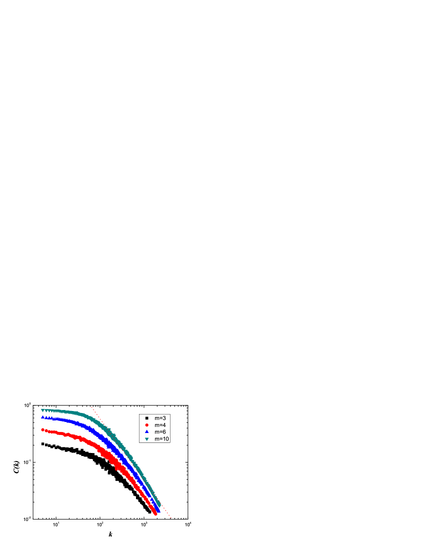
Figure 8: The clustering coefficient $C(k)$ depending on connectivity $k$ for increasing $m$. For comparison, the dashed line has slope -1 in the log-log scale.

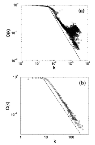
Figure 9: The scaling of $C(k)$ with $k$ for two real networks hierarchy : (a)Actor network, two actors being connected if they acted in the same movie according to the www.IMDB.com database. (b)The semantic web, connecting two English words if they are listed as synonyms in the Merriam Webster dictionary. The dashed line in each figure has slope -1.

Another important source of information is the correlations of the degree of neighboring vertices. The average nearest neighbor degree is proposed to measure these correlations

$$k_{nn,i}=\frac{1}{k_{i}}\sum_{j}a_{ij}k_{j}.$$ (14)

Once averaged over classes of vertices with connectivity $k$, the average nearest neighbor degree can be expressed as

$$k_{nn}(k)=\sum_{k^{\prime}}P(k^{\prime}|k),$$ (15)

providing a probe on the degree correlation function. If degrees of neighboring vertices are uncorrelated, $P(k^{\prime}|k)$ is only a function of $k^{\prime}$ and thus $k_{nn}(k)$ is a constant. When correlations are present, two main classes of possible correlations have been identified: assortative behavior if $k_{nn}(k)$ increases with $k$, which indicates that large degree vertices are preferentially connected with other large degree vertices, and disassortative if $k_{nn}(k)$ decreases with $k$. The above quantities provide clear signals of a structural organization of networks in which different degree classes show different properties in the local connectivity structure. In the light of this measure, we also perform computer simulations to test the $k_{nn}(k)-k$ correlation, as shown in Fig. 10. As $k_{nn}(k)$ decreases with $k$, one may find that our model can best illustrate disassortative networks in reality, that mainly is, technological networks (e.g. Internet, WAN) and biological networks (e.g. Protein Folding Networks). As for the social networks, connections between people may be assortative by language or by race. Newman proposed some simpler measures to describe these types of mixing, which we call assortativity coefficients mixing . Almost all the social networks studied show positive assortativity coefficients while all others, including technological and biological networks, show negative coefficients. It is not clear if this is a universal property; the origin of this difference is not understood either. In our views, it represents a feature that should be addressed in each network type individually. In the following, we use the formula proposed by Newman in Ref. mixing ,

$$r=\frac{M^{-1}\sum_{i}j_{i}k_{i}-[M^{-1}\sum_{i}\frac{1}{2}(j_{i}+k_{i})]^{2}}{M^{-1}\sum_{i}\frac{1}{2}(j_{i}^{2}+k_{i}^{2})-[M^{-1}\sum_{i}\frac{1}{2}(j_{i}+k_{i})]^{2}},$$ (16)

where $j_{i}$, $k_{i}$ are the degrees of vertices at the ends of the $i$th edges, with $i=1,...,M$ ($M$ is the total number of edges in the observed graph). We calculate the degree assortativity coefficient (or degree-degree correlation) $r$ of the graphs generated by our model. For large $N$ (e.g. $N>5000$), the degree-degree correlation $r$ is almost independent of the network size (see Fig. 11). Simulations of $r$ depending on $m$ are given in Fig. 12 and supported by empirical measurements for disassortative networks mixing .

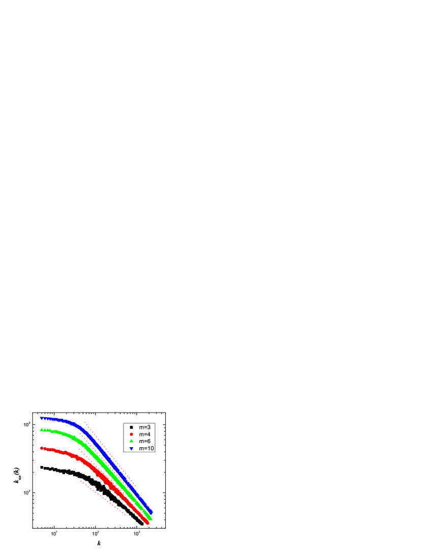
Figure 10: Average connectivity $k_{nn}(k)$ of the nearest neighbors of a node depending on its connectivity $k$ for different $m$.

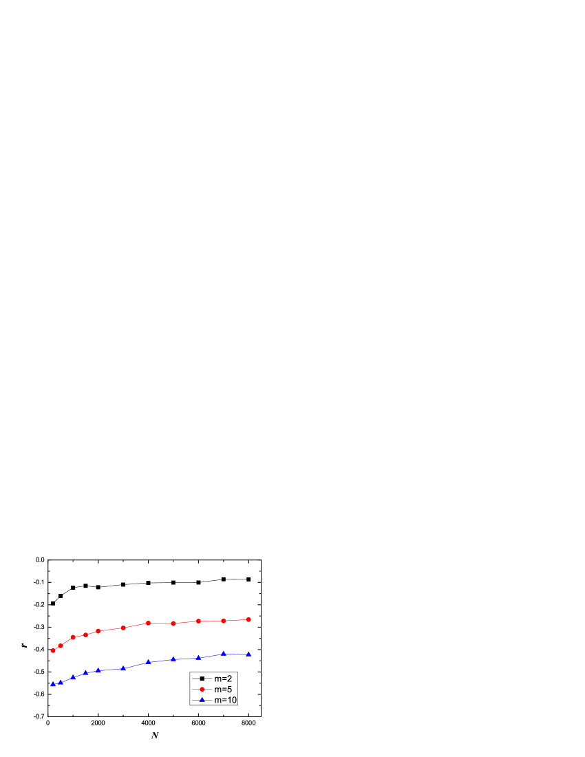
Figure 11: Degree-degree correlation $r$ depending on $N$. The evolution of $r$ converges soon.

Figure 12: Degree-degree correlation $r$ depending on $m$.

V Conclusion and outlook

In sum, integrating the mutual selection mechanism between nodes and the growth of strength preferential attachment, our network model provides a wide variety of scale-free behaviors, tunable clustering coefficient and nontrivial (degree-degree and strength-degree) correlations, just depending on the parameter $m$ which governs the total weight growth. All the results of network properties are found supported by various empirical data. Interestingly and specially, studying the degree-dependent average clustering coefficient $C(k)$ and the degree-dependent average nearest neighbors’ degree $k_{nn}(k)$ also provide us with a better description of the hierarchies and organizational architecture of weighted networks. As far as our knowledge, there at present appears no model that could generate so many properties which are in broad agreement with empirical data. Thus, our model may be very beneficial for future understanding or characterizing real networks. Though our model can just produce disassortative networks (most suitable for technological and biological ones), which means one of its limitations, we always expect some model versions or variations that generate weighted networks with assortative property. Due to the apparent simplicity of our model and the variety of tunable results, we believe that some of its extensions will probably help address (e.g. social) networks. Therefore, our present model for all practical purposes will demonstrate its applications in future weighted network research.

- (1) R. Pastor-Satorras and A. Vespignani, Evolution and Structure of the Internet: A Statistical Physics Approach (Cambridge University Press, Cambridge, England, 2004).
- (2) R. Albert, H. Jeong, and A.-L. Barabási, Nature 401, 130 (1999).
- (3) M.E.J. Newman, Phys. Rev. E 64, 016132 (2001).
- (4) A.-L. Barabási, H. Jeong, Z. Néda. E. Ravasz, A. Schubert, and T. Vicsek, Physica (Amsterdam) 311A, 590 (2002).
- (5) M. Li, J. Wu, D. Wang, T. Zhou, Z. Di and Y. Fan, arXiv: cond-mat/0501655.
- (6) R. Guimera, S. Mossa, A. Turtschi, and L.A.N Amearal, cond-mat/0312535.
- (7) A. Barrat, M. Barthélemy, R. Pastor-Satorras, and A. Vespignani, Proc. Natl. Acad. Sci. U.S.A. 101, 3747 (2004).
- (8) W. Li and X. Cai, Phys. Rev. E 69, 046106(2004).
- (9) R. Albert and A.-L. Barabási, Rev. Mod. Phys. 74, 47 (2002).
- (10) A. Barrat, M. Barthélemy, and A. Vespignani, Phys. Rev. Lett. 92, 228701 (2004).
- (11) C. Li and G. Chen, cond-mat/0309236.
- (12) K.-I. Goh, B. Kahng, and D. Kim, cond-mat/0410078 (2004).
- (13) R. Pastor-Satorras, A. Vázquez, and A. Vespignani, Phys. Rev. Lett. 87, 258701(2001).
- (14) A. Vázquez, R. Pastor-Satorras and A. Vespignani, Phys. Rev. E 65, 066130(2002).
- (15) E. Ravasz and A.-L Barabási, Phys. Rev. E textbf67, 026112 (2003).
- (16) S.N. Dorogovtsev and J.F.F. Mendes, Europhys. Lett. 50, 33 (2000).
- (17) S.H. Yook, H. Jeong, A.-L. Barabási, and Y. Tu, Phys. Rev. Lett. 86, 5835 (2001).
- (18) D. Zheng, S. Trimper, B. Zheng, and P.M. Hui, Phys. Rev. E 67, 040102 (2003).
- (19) P. Holme and B. J. Kim, Phys. Rev. E 65 066109(2002).
- (20) T. Zhou, G. Yan, P. -L. Zhou, Z. -Q. Fu and B. -H. Wang, arXiv: cond-mat/0409414.
- (21) T. Zhou, G. Yan and B. -H. Wang, arXiv: cond-mat/0412448(Phys. Rev. E In Press).
- (22) M. E. J. Newman, Phys. Rev. E 67, 026126 (2003).