Anisotropy of the upper critical field in MgB₂: the two-gap Ginzburg-Landau theory

Abstract

The upper critical field in MgB₂ is investigated in the framework of the two-gap Ginzburg-Landau theory. A variational solution of linearized Ginzburg-Landau equations agrees well with the Landau level expansion and demonstrates that spatial distributions of the gap functions are different in the two bands and change with temperature. The temperature variation of the ratio of two gaps is responsible for the upward temperature dependence of in-plane $H_{c2}$ as well as for the deviation of its out-of-plane behavior from the standard angular dependence. The hexagonal in-plane modulations of $H_{c2}$ can change sign with decreasing temperature.

1 Introduction

Multigap superconductivity suhl ; moskalenko has been discussed in the late 1950’s for materials with a varying strength of electron-phonon interactions between different pieces of the Fermi surface. After the discovery of superconductivity in MgB₂ akimitsu in 2001, an impressive collection of experimental and theoretical works review has established that this compound is the first unambiguous example of a multigap superconductor. In MgB₂ the charge carriers are distributed between two sets of bands: the $\sigma$-bands with quasi-2D cylindrical Fermi sheets and the $\pi$-bands with 3D sheets forming a tubular network. The electron-phonon coupling is stronger in the $\sigma$-bands than in the $\pi$-bands, and gives rise to an $s$-wave phonon-mediated superconductivity with two gaps $\Delta_{1}\sim 7$ meV and $\Delta_{2}\sim 2.5$ meV. Since the two sets have different characteristics (interaction with phonons, geometry of the Fermi sheets, impurity dependence etc.), an interplay between them results in deviations from the standard BCS theory. The most striking consequences of the two gaps are the unusual anisotropic features of MgB₂ under magnetic field, for example, inequality between the penetration depth and the upper critical field anisotropies, and their variations with temperature angst ; samuely ; cubitt1 ; shi ; rydh ; golubov1 ; golubov2 ; miranovic ; kogan ; dahm ; gurevich ; kita , and the 30^∘-reorientation of the flux line lattice with increasing magnetic field applied along the $c$-axis cubitt2 ; zhitomirsky .

The two-gap Ginzburg-Landau (GL) theory for MgB₂ developed in Ref. zhitomirsky (see also the preceding works tilley ; geilikman ) is the exact limit of the microscopic theory in the vicinity of the transition temperature. It can thus account for most of the observed properties in a clear and coherent way near $T_{c}$, while its simplicity compared to earlier studies is useful to understand the physics in this material. In the present paper we extend our previous analysis of the two-band effects zhitomirsky on angular and temperature dependence of the upper critical field $H_{c2}$. We minimize the GL functional using a variational procedure, which highlights separate spatial anisotropies of the gap in each band. This is an improvement compared to the earlier solutions where only one common distortion for both gaps is considered golubov2 ; dahm . This method is compared to a solution based on the Landau level expansion. We then estimate the temperature range of the GL regime. The present study covers the out-of-plane $H_{c2}$ anisotropy. By going beyond the ellipsoid Fermi sheet approximation of Refs. miranovic ; dahm , we also calculate in-plane modulation of the upper critical field arising from the hexagonal crystal symmetry.

For a clean two-band BCS superconductor with two gaps $\Delta_{1}$ and $\Delta_{2}$, the GL functional zhitomirsky has the form

$$F_{GL}=\int dx\Bigl{[}\alpha_{1}|\Delta_{1}|^{2}+\alpha_{2}|\Delta_{2}|^{2}-\gamma(\Delta_{1}^{*}\Delta_{2}+\Delta_{2}^{*}\Delta_{1})$$

$$\mbox{}\!+K_{1i}|\Pi_{i}\Delta_{1}|^{2}\!+K_{2i}|\Pi_{i}\Delta_{2}|^{2}+\textstyle\frac{1}{2}\beta_{1}|\Delta_{1}|^{4}\!+\textstyle\frac{1}{2}\beta_{2}|\Delta_{2}|^{4}\!\Bigr{]},$$

$$\Pi_{i}=-i\partial_{i}+\frac{2\pi}{\Phi_{0}}A_{i},\ \ \alpha_{1,2}=\frac{g_{2,1}}{G}-N_{1,2}\ln\frac{2\omega_{D}e^{C}}{\pi T},$$

$$\gamma=\frac{g_{3}}{G},\ \ K_{ni}=\frac{7\zeta(3)N_{n}}{16\pi^{2}T_{c}^{2}}\langle v_{Fni}^{2}\rangle,\ \ \beta_{n}=\frac{7\zeta(3)N_{n}}{8\pi^{2}T_{c}^{2}}$$ (1)

where repeating index $i$ implies a sum, $\Phi_{0}$ is the quantum flux, $\bf A$ the potential vector, $g_{1}$ and $g_{2}$ the intraband pairing coefficients ($n$=1,2 for the $\sigma$,$\pi$-band), $g_{3}$ the interband pairing coefficient, $G=g_{1}g_{2}-g_{3}^{2}$, $N_{n}$ the density of states at the Fermi level in the band $n$, $\omega_{D}$ the Debye frequency, C the Euler constant, and $\langle v_{Fni}^{2}\rangle$ the square of the Fermi velocity $i$-component averaged on the sheet $n$. It is then convenient to write $\alpha_{1}=-a_{1}t$ with $a_{1}=N_{1}$, $t=\ln(T_{1}/T)$ and $T_{1}=(2\omega_{D}e^{C}/\pi)e^{-g_{2}/GN_{1}}$ for the first active band and $\alpha_{2}=\alpha_{20}-a_{2}t$ with $a_{2}=N_{2}$ for the passive band. In MgB₂ the active and passive bands correspond to the $\sigma$ and $\pi$ bands, respectively.

The crystal structure of MgB₂ is uniaxial, so the gradient coefficients are the same for all directions in the basal plane, and $K_{na}=K_{nb}=K_{n}$. LDA calculations kong yield for the highly anisotropic $\sigma$-band $\langle v_{F1ab}^{2}\rangle=2.13$ and $\langle v_{F1c}^{2}\rangle=0.05$, while for the $\pi$-band $\langle v_{F2ab}^{2}\rangle=1.51$ and $\langle v_{F2c}^{2}\rangle=2.96$, all numbers are in units of $10^{15}$ cm²/s². With the provided ratio $N_{2}/N_{1}=1.5$, the in-plane gradient constants for the two bands are practically the same $K_{2}/K_{1}\approx 1.06$, whereas the $c$-axis constants differ by almost two orders of magnitude $K_{2c}/K_{1c}\approx 90$. A crude estimate for $H_{c2}$ at zero temperature by $\frac{N_{1}}{\sqrt{K_{1}K_{1c}}}\frac{\Phi_{0}}{2\pi}\approx 4$T is substantially smaller than the experimental value $H_{c2}^{ab}(0{\rm K})\approx 18$T, which suggests the gradient constants based on LDA data are over-estimated by a factor of four. Such a discrepancy is due to a significant renormalization of effective masses by the electron-phonon coupling. The electron-phonon coupling leads to effective masses twice larger than the LDA prediction in the $\sigma$-band, whereas they are only slightly renormalized in the $\pi$-band mazin . The reduction of gradient term coefficients is given by squares of the mass renormalization factors.

The interband impurity scattering in MgB₂ is exceptionally small due to its particular electronic structure, even in low quality samples mazin2 . The clean limit two-gap GL theory described above is straightforwardly extended to include the effect of s-wave intraband scattering by non-magnetic impurities pokrovsky : the GL functional keeps the same form wherein the expression for $K_{ni}$ has to be replaced by $K_{ni}=\pi N_{n}\langle v_{Fni}^{2}\rangle\Lambda(\tau_{n})/8T_{c}$ with

$$\Lambda(\tau_{n})=\tau_{n}\frac{8}{\pi^{2}}\sum_{m}\frac{1}{(2m+1)^{2}((2m+1)2\pi\tau_{n}T_{c}+1)}\ ,$$ (2)

where $\tau_{n}$ is the transport collision time in the band $n$. The intraband anisotropy is then the same as in the clean limit, while the renormalization factor $\Lambda(\tau_{n})$ can vary between the two bands due to different sensitivity to impurities. The resulting GL equations are naturally found as the limit of Usadel equations near $T_{c}$. golubov2 ; gurevich .

2 Upward curvature of $H_{c2}^{ab}(T)$

In this section the $z$-axis is fixed along the crystal $c$-axis and the $y$-axis is taken parallel to the magnetic field applied in the $ab$-plane. The vector potential is chosen in the Landau gauge as ${\bf A}=(Hz,0,0)$. The coupled linearized GL equations for solutions homogeneous along the field direction are

$$\left(\alpha_{n}+K_{n}h^{2}z^{2}-K_{nc}\partial_{z}^{2}\right)\Delta_{n}-\gamma\Delta_{n^{\prime}}=0$$ (3)

for $n=1,2$, $n^{\prime}=2,1$, with the reduced magnetic field $h=2\pi H/\Phi_{0}$. Since $K_{1c}/K_{1}\neq K_{2c}/K_{2}$, an analytic solution can not be obtained by rescaling distances as in the single-gap case. We, therefore, search for an approximate solution of the form

$$\left(\begin{array}[]{c}\Delta_{1}\\ \Delta_{2}\end{array}\right)=\left(\begin{array}[]{c}c\;\tilde{\xi}_{1}^{-\frac{1}{2}}\Psi_{0}(z/\tilde{\xi}_{1})\\ d\;\tilde{\xi}_{2}^{-\frac{1}{2}}\Psi_{0}(z/\tilde{\xi}_{2})\end{array}\right)$$ (4)

where the Landau level wave functions are defined by

$$\Psi_{p}(z)=\frac{1}{\sqrt{p!}}\left[\frac{1}{\sqrt{2}}(-\partial_{z}+z)\right]^{p}\frac{e^{-z^{2}/2}}{\pi^{1/4}}$$ (5)

Different coherence lengths for each band are allowed with the parameterization $\tilde{\xi}_{n}^{2}=\mu_{n}/h$ where $\mu_{n}$ quantifies the distortion of the spatial distribution of the $n$-th component (in the single-gap case, $\mu$ is the stretching factor of the flux line lattice at the upper critical field and is independent from temperature). The following quadratic form in the GL functional is then found:

$$F_{2} = (\alpha_{1}+h\tilde{K}_{1})|c|^{2}+(\alpha_{2}+h\tilde{K}_{2})|d|^{2}$$ (6)

$$-\tilde{\gamma}(c^{*}d+d^{*}c)$$

with $\tilde{K}_{n}=\textstyle\frac{1}{2}(K_{n}\mu_{n}+K_{nc}/\mu_{n})$ and $\tilde{\gamma}^{2}=\gamma^{2}\frac{2\sqrt{\mu_{1}\mu_{2}}}{\mu_{1}+\mu_{2}}$. At the transition field, the determinant in Eq. (6) vanishes. This condition leads to

$$\tilde{h}(\mu_{1},\mu_{2})=-\frac{\alpha_{1}}{2\tilde{K}_{1}}-\frac{\alpha_{2}}{2\tilde{K}_{2}}+\sqrt{\left(\frac{\alpha_{1}}{2\tilde{K}_{1}}-\frac{\alpha_{2}}{2\tilde{K}_{2}}\right)^{2}\!+\frac{\tilde{\gamma}^{2}}{\tilde{K}_{1}\tilde{K}_{2}}}$$ (7)

In order to find the (nucleation) upper critical field, $\tilde{h}$ is maximized $\tilde{h}_{c2}=\max_{\mu_{1},\mu_{2}}\;\tilde{h}(\mu_{1},\mu_{2})$.

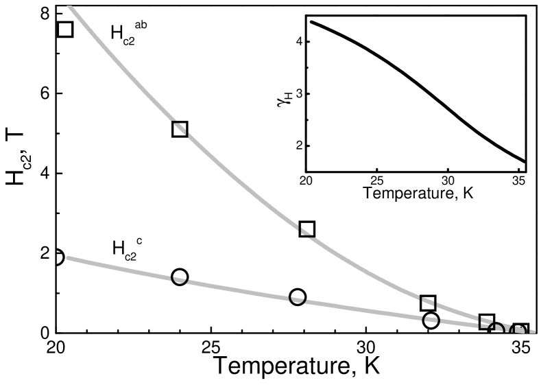
Figure 1: The upper critical field in MgB₂: experimental data from Lyard et al. samuely (symbols) and the GL computations with parameters $\alpha_{20}=0.65a_{1}$ and $\gamma=0.4a_{1}$ (solid lines). The inset shows the anisotropy ratio $\gamma_{H}=H_{c2}^{ab}/H_{c2}^{c}$.

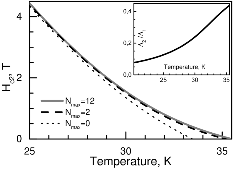
Figure 2: In-plane $H_{c2}$ calculated with the Landau level expansion to the order $N_{\rm max}$ for the same parameters as in Fig. 1. The inset displays the gap ratio $\rho=\Delta_{2}/\Delta_{1}$ found with the highest expansion order.

Within the above variational scheme, the analytic expressions for the in-plane transition field are possible in two temperature regimes. Near $T_{c}$, vanishing $\tilde{h}$ implies that the superconducting gaps have the same variation length in each band. The condition $\mu_{1}=\mu_{2}$ yields

$$\tilde{h}^{ab}_{c2}\approx\frac{a_{1}(t-t_{c})}{\sqrt{(K_{1}+\rho^{2}K_{2})((K_{1z}+\rho^{2}K_{2z})}}$$ (8)

with the gap ratio $\rho=|d/c|\approx\sqrt{\alpha_{1}/\alpha_{2}}$ and $t_{c}=\ln(T_{1}/T_{c})$. Since $K_{1c}\sim 0.01K_{2c}$ in MgB₂, whereas $\rho^{2}\approx 0.1$, we can simplify the above expression to

$$\tilde{h}^{ab}_{c2}\approx\frac{a_{1}(t-t_{c})}{\rho\sqrt{K_{1}K_{2c}}}\;.$$ (9)

In the second temperature regime for $T<T_{1}$, the first active band is dominant and

$$\tilde{h}^{ab}_{c2}\approx\frac{a_{1}t}{\sqrt{K_{1}K_{1c}}}\;.$$ (10)

The line $H^{ab}_{c2}(T)$ exhibits, therefore, a marked upturn curvature between the two regimes, in contrast to $H_{c2}^{c}$(T). The two upper critical fields are plotted in Fig. 1. In order to fit the experimental data, we have renormalized all gradient constants obtained from the LDA data by a factor of five. The corresponding mass enhancement $\sqrt{5}\approx 2.2$ roughly agrees with the electron-phonon renormalization factormazin . For simplicity, the same value has been applied for both bands.

In order to verify an accuracy of the variational method, we alternatively proceed by expanding the gap functions in terms of the the Landau levels: $\Delta_{n}=\sum_{p}c_{n,p}\phi_{n,p}$ where $\phi_{n,p}(z)=\xi_{n}^{-1/2}\Psi_{p}(z/\xi_{n})$ and $\xi_{n}^{2}=\sqrt{K_{nc}/K_{n}}/h$. For the upper critical field this expansion is restricted to the even order levels. The quadratic part of the GL functional has the following matrix element in this base:

$$M^{F_{2}}_{2p+n,2q+n^{\prime}}=\left(\alpha_{n}+(4p+1)h\sqrt{K_{n}K_{nc}}\right)\delta_{n,n^{\prime}}\delta_{p,q}$$

$$-\gamma\int\!\!dx\;\phi_{n,2p}^{*}(x)\phi_{n^{\prime},2q}(x)\;(1-\delta_{n,n^{\prime}})$$ (11)

with $n,n^{\prime}\in\{1,2\}$, and $p,q\geq 0$. The upper critical field $h_{c2}$ is then approximated by the largest root of the sub-matrix determinant corresponding to the desired expansion up to the order $N_{\rm max}$.

Although the zeroth order approximation significantly deviates near $T_{c}$ (see Fig. 2), the procedure is rapidly converging with increasing the expansion order, even in the case of a great disparity between the two bands (e.g., $\xi_{1}^{2}/\xi_{2}^{2}\geq 100$ or $\leq 0.01$). The expansion to the order $N_{\rm max}\geq 12$ yields the upper critical field curve in excellent agreement with the variational solution (the two curves are indistinguishable on the scale of Fig. 2).

Fig. 3 displays the behavior of the parameters $\mu_{n}$ defining the effective anisotropy of the variation lengths $\tilde{\xi}_{n}$ in the plane perpendicular to the magnetic field, i. e. $\mu_{n}=\tilde{\xi}_{nc}/\tilde{\xi}_{nab}$ for the magnetic field applied in the basal plane. This confirms the above analytic predictions: the order parameter varies on different length scales for each band, and $\mu_{n}$ can change with temperature contrary to the single-gap case. At $T_{c}$, the two parameters have the same value $\sqrt{(K_{1z}+\rho^{2}K_{2z})/(K_{1}+\rho^{2}K_{2})}=0.59$ with $\rho=0.44$, while $\mu_{1}\approx\sqrt{K_{1c}/K_{1}}=0.15$ below $T_{1}=29$ K. We should stress that periodic vortex structures for the two gaps have the same lattice parameters for arbitrary ratio of $\mu_{1}/\mu_{2}$. However, spatial distributions of $|\Delta_{1}(r)|^{2}$ and $|\Delta_{2}(r)|^{2}$ become quite different at low temperatures once $\mu_{1}\ll\mu_{2}$. Such a behavior is demonstrated on the top panel of Fig. 3. The different spatial distributions of the two gaps can be probed by scanning tunneling microscopy. Also, magnetic field generated by superconducting currents $h_{s}(r)\sim(|\Delta_{1}(r)|^{2}+|\Delta_{2}(r)|^{2})$ should deviate significantly for a distribution expected for an anisotropic single-gap superconductor. Muon spin relaxation measurements can in principle verify such a behavior.

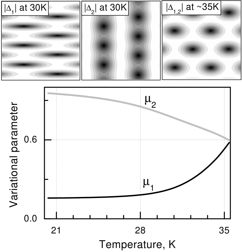
Figure 3: Lower panel: temperature dependence of variational parameters for in-plane magnetic field and the same set of GL parameters as in Fig. 1; Upper panel: absolute values of the two gaps in the vicinity of $H_{c2}$ near to and away from the transition temperature.

We shall now estimate the temperature range of the GL regime from the above computations. The gradient expansion is valid as long as $|K_{ni}\partial_{i}^{2}\Delta_{n}|<\Delta_{n}$ for all $n$ and $i$. This condition is approximately replaced with $K_{ni}/\tilde{\xi}^{2}_{ni}<1$. The most restrictive case is for $K_{2c}/\tilde{\xi}^{2}_{2c}=K_{2c}h_{c2}^{ab}/\mu_{2}$, which becomes $\sim 1$ below $\sim 30$ K, well beyond a narrow temperature regime suggested for the GL theory by Golubov and Koshelev golubov2 . The discrepancy is partially terminological, since in Ref. golubov2 the GL approximation always corresponds to an effective (anisotropic) single-gap GL theory, which is correct only when the ratio of the two gaps is constant. As we have demonstrated above, the full two-gap GL theory is valid in a much wider temperature range and describes adequately temperature variation of $\Delta_{2}/\Delta_{1}$ (Fig. 2) and of the two coherence lengths (Fig. 3).

3 Angular dependence of out-of-plane $H_{c2}$

Let us now discuss the out-of-plane behavior of the upper critical field. In the single-gap anisotropic GL theory, when ${\bf H}$ is tilted from the c-axis by an angle $\theta$, the upper critical field has an elliptic (effective mass) angular dependence

$$H_{\rm SAGL}(\theta,T)=\frac{H_{c2}^{c}(T)}{\sqrt{\cos^{2}(\theta)+\sin^{2}(\theta)\gamma_{H}^{-2}}}\ ,$$ (12)

where $\gamma_{H}=H^{ab}_{c2}/H^{c}_{c2}$ is a temperature independent constant $\sqrt{K_{c}/K_{ab}}$. Experimental measurements in MgB₂ have shown that not only $\gamma_{H}$ changes with temperature (Fig. 1) but deviations from the elliptic angular dependence (12) grow with decreasing temperature angst ; shi ; rydh . Such a behavior has been reproduced within quasi-classical Usadel equations golubov2 . The methods we have employed for $H_{c2}^{ab}$ are still valid to find $H_{c2}(\theta)$: one needs only to replace $K_{nc}$ by an angular dependent $K_{n}(\theta)=\cos^{2}(\theta)K_{n}+\sin^{2}(\theta)K_{nc}$ in the previous formula. Expression (7) for $\tilde{h}$ shows that the deviation grows with the disparity between the $\tilde{K}_{n}(\theta)$, so it increases when departing from $T_{c}$. The deviations can be quantified by $\delta A(\theta)=1-(H_{c2}(\theta)/H_{\rm SAGL}(\theta))^{2}$. Fig. 4 displays the maximum deviation $\delta A_{\rm max}={\rm max}_{\theta}\delta A(\theta)$. The dashed line is obtained from the two-gap GL theory with the parameters used above to fit the $H_{c2}$-data by Lyard et al.samuely in Fig. 1. The calculation qualitatively reproduces experimental data from Rydh et al. rydh : $\delta A_{\rm max}$ increases with decreasing temperature and then saturates. But a quantitative discrepancy appears below $0.9T_{c}$ and becomes important at lower temperature. This deviation can be partially explained by the fact that experimental results are strongly sample dependent. At the present, the origin of the discrepancy remains an opened question. The full line is obtained with a modified interband coupling $\gamma^{\star}=0.3a_{1}$ and $K_{c2}^{\star}=K_{2c}/3$ corresponding to a smaller anisotropy in the $\pi$-band.

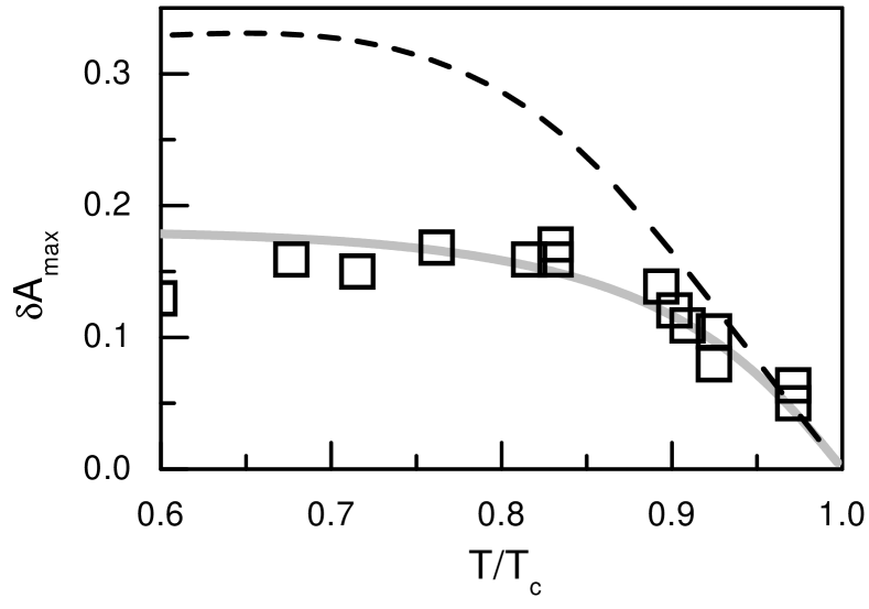
Figure 4: Maximum deviation from the single-gap GL scaling law : squares are experimental data rydh and lines are obtained from the two-gap GL theory.

4 In-plane modulation of $H_{c2}$

In a hexagonal crystal, the transition magnetic field should exhibit a six-fold modulation when rotated about the $c$-axis skokan . The crystal field effect on superconductivity can be incorporated to the GL theory by including higher order (non-local) gradient terms hohenberg . Symmetry arguments suggest that coupling between the superconducting order parameter and the hexagonal crystal lattice appears at the sixth-order gradient terms. For a two-gap superconductor like MgB₂, the additional sixth-order part of the free energy is a sum of separate contributions from each band: $F_{GL}\longrightarrow F_{GL}+F_{6,1}+F_{6,2}$. The correction derived from the BCS theory zhitomirsky ; takanaka is (omitting the index $n=1,2$ for brevity)

$$F_{6} = \frac{\zeta(7)N}{32\pi^{6}T_{c}^{6}}\left(1-\frac{1}{2^{7}}\right)\langle v_{Fi}v_{Fj}v_{Fk}v_{Fl}v_{Fm}v_{Fn}\rangle$$ (13)

$$\mbox{}\times(\Pi_{i}\Pi_{j}\Pi_{k}\Delta)^{*}(\Pi_{l}\Pi_{m}\Pi_{n}\Delta)\ .$$

Setting the $z$-axis perpendicular to the basal plane, the above terms can be split into isotropic in-plane part

$$F_{6}^{\rm iso}=K_{6}^{i}\Delta^{*}\Bigl{[}\Pi_{x}^{2}+\Pi_{y}^{2}\Bigr{]}^{3}\Delta$$ (14)

with $K_{6}^{i}=\frac{\zeta(7)N}{64\pi^{6}T_{c}^{6}}\left(1-\frac{1}{2^{7}}\right)\bigl{(}\langle v_{Fx}^{6}\rangle+\langle v_{Fy}^{6}\rangle\bigr{)}$, and anisotropic in-plane contribution

$$F_{6}^{\rm an}=\frac{1}{2}K_{6}^{a}\Delta^{*}\Bigl{[}(\Pi_{x}+i\Pi_{y})^{6}+(\Pi_{x}-i\Pi_{y})^{6}\Bigr{]}\Delta$$ (15)

with $K_{6}^{a}=\frac{\zeta(7)N}{64\pi^{6}T_{c}^{6}}\left(1-\frac{1}{2^{7}}\right)\bigl{(}\langle v_{Fx}^{6}\rangle-\langle v_{Fy}^{6}\rangle\bigr{)}$. This expression of $F^{\rm an}_{6}$ assumes that the $x$- and the $y$-axes are parallel to the reflection lines in the $ab$-plane. With the $x$-axis parallel to the $b$-direction, tight-biding calculationszhitomirsky yield $\langle v_{Fx}^{6}\rangle=4.608$, $\langle v_{Fy}^{6}\rangle=4.601$ for the $\sigma$-band, while for the $\pi$-band, $\langle v_{Fx}^{6}\rangle=1.514$, $\langle v_{Fy}^{6}\rangle=1.776$ in units of $10^{46}$ (cm/s)⁶. The different sign of the hexagonal harmonics of the Fermi velocities in the two bands is responsible for a unique $30$-degree orientational transition of the vortex lattice in MgB₂.zhitomirsky No theory can describe at present the electron-phonon effect on the hexagonal modulation of the Fermi surface. We use, therefore, the raw LDA values for all gradient coefficients in the consideration below. If we rotate now the orthogonal axes so that the $y$-axis is parallel to the magnetic field ${\bf H}$ when the latter forms an angle $\phi$ with the $a$-axis, the terms in $F_{6}$ change in a simple way: $F_{6}^{\rm iso}$ is preserved while $F_{6}^{\rm an}$ turns into

$$F_{6}^{\rm an}=\frac{1}{2}K_{6}^{a}\Delta^{*}\Bigl{[}e^{i6\phi}(\Pi_{x}+i\Pi_{y})^{6}+e^{-i6\phi}(\Pi_{x}-i\Pi_{y})^{6}\Bigr{]}\Delta\$$ (16)

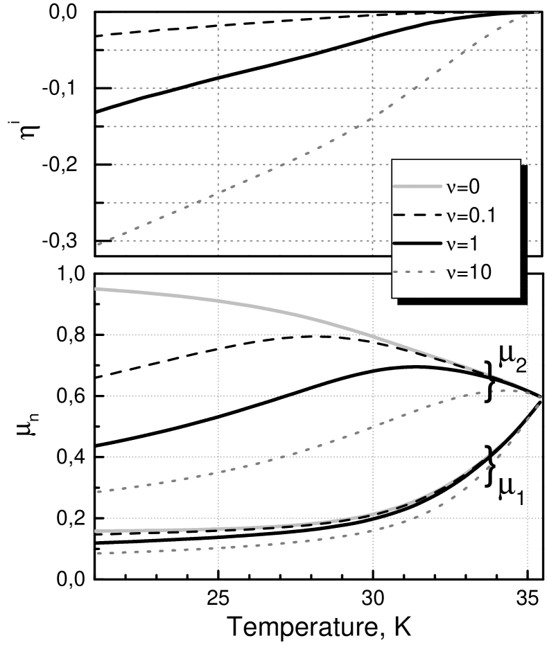
Figure 5: Influence of the isotropic correction $F_{6}$ with $(\langle v_{F1}^{6}\rangle,\langle v_{F2}^{6}\rangle)=\nu(4.6,1.6)$ (in units of $10^{46}$ (cm/s)⁶) for different magnitudes $\nu$: relative shift of the upper critical field $\eta^{i}=(H_{c2}^{\nu}-H_{c2}^{\circ})/H_{c2}^{\circ}$ and corresponding variational parameters $\mu_{n}$.

Since $\Pi_{y}=0$, the extra term can be written as $F_{6}=\sum K_{6,n}\Delta_{n}^{*}\Pi_{x}^{6}\Delta_{n}$ with $K_{6,n}=K_{6,n}^{i}+K_{6,n}^{a}\cos(6\phi)$. For the variational approximation, the new functional yields the quadratic form

$$F_{2} = (\alpha_{1}+\tilde{K}_{1}h+\tilde{K}_{6,1}h^{3})|c|^{2}+(\alpha_{2}+\tilde{K}_{2}h$$ (17)

$$+\tilde{K}_{6,2}h^{3})|d|^{2}-\tilde{\gamma}(c^{*}d+d^{*}c)$$

with $\tilde{K}_{6,n}=\frac{15}{8}K_{6,n}\mu_{n}^{3}$. While in the expansion method, this results in the new matrix element

$$M^{F_{2}+F_{6}}_{2p+n,2q+n^{\prime}}=M^{F_{2}}_{2p+n,2q+n^{\prime}}+h^{3}K_{6,n}\left(\frac{K_{nc}}{K_{n}}\right)^{\!\!3/2}\!\!\!\!M^{(6)}_{2p,2q}\delta_{n,n^{\prime}}$$ (18)

with $M^{(6)}_{p,q}=\frac{1}{8}\left\langle\Psi_{p}|(\hat{a}^{\dagger}+\hat{a})^{6}|\Psi_{q}\right\rangle$ where $\hat{a}$ is the annihilation operator of Landau levels.

In the weakly anisotropic regime $F_{6}<\!\!<F_{2}$, we expect

$$H_{c2}(\phi)\approx H_{c2}^{\circ}\left(1+\eta^{i}+\eta^{a}\cos(6\phi)\right)$$ (19)

The isotropic parts yield a $\phi$-independent shift of $H_{c2}$ (and ensure $K_{6,n}>0$ for the numerical solution converging) while the anisotropic parts are responsible for the six-fold modulation of the correction. $\eta^{a}$ can change sign when the temperature varies because the anisotropies in each band are opposite. Fig. 5 displays the corrections brought by the isotropic parts of $F_{6}$. The deviations become important below 30K as expected out of the estimated GL regime, which implies the necessity to retain higher order terms in the gradient expansion of the GL functional.

The extra $h^{3}$ terms prevent from deriving an analytical expression for the magnetic field correction $\delta h_{c2}=h_{c2}(\phi)-h_{c2}(\pi/12)$. We can however partially estimate the latter. Let us name the quantities related to the quadratic form $(F_{2}+F_{6}^{\rm iso})$ with the superscript ”$\circ$”, and the ones for $(F_{2}+F_{6}^{\rm iso}+F_{6}^{\rm an})$ without it. Within the variational method, we then find with a perturbation expansion

$$\frac{\delta\tilde{h}_{c2}}{\tilde{h}^{\circ}_{c2}} \approx \frac{1}{\tilde{h}^{\circ}_{c2}}\frac{d\tilde{h}^{\circ}_{c2}}{dT}\left.\frac{\langle\Delta^{\circ}|F_{6}^{\rm an}|\Delta^{\circ}\rangle}{\langle\Delta^{\circ}|\partial(F_{2}+F_{6}^{\rm iso})/\partial T|\Delta^{\circ}\rangle}\right|_{\tilde{h}_{c2}^{\circ}}$$

$$\approx \frac{15}{8}\cos(6\phi)T\frac{d\tilde{h}^{\circ}_{c2}}{dT}\tilde{h}_{c2}^{{\circ}\;\stackrel{{\scriptstyle\scriptstyle 2}}{{\;}}}\frac{K_{6,1}^{a}\mu_{1}^{{\circ}\;\stackrel{{\scriptstyle\scriptstyle 3}}{{\;}}}+K_{6,2}^{a}\mu_{2}^{{\circ}\;\stackrel{{\scriptstyle\scriptstyle 3}}{{\;}}}\rho^{2}}{a_{1}+a_{2}\rho^{2}}$$

where $\rho^{2}=|c^{\circ}/d^{\circ}|^{2}$. The expansion method provides in a similar way

$$\frac{\delta h_{c2}}{h^{\circ}_{c2}}\approx\frac{T}{h^{\circ}_{c2}}\frac{dh^{\circ}_{c2}}{dT}\left.\frac{(1+\rho^{2})\langle\Delta^{\circ}|F_{6}^{\rm an}|\Delta^{\circ}\rangle}{a_{1}+a_{2}\rho^{2}}\right|_{h_{c2}^{\circ}}$$ (21)

but $\langle\Delta^{\circ}|F_{6}^{\rm an}|\Delta^{\circ}\rangle$ has a more complicated expression.

In Fig. 6, we have plotted the relative modulation amplitude $\eta^{a}=(h_{c2}(0)-h_{c2}(\pi/6))/(h_{c2}(0)+h_{c2}(\pi/6))$ with the hexagonal anisotropy $\langle v_{Fb}^{6}\rangle=\langle v_{F}^{6}\rangle^{i}+\langle v_{F}^{6}\rangle^{a}$ and $\langle v_{Fa}^{6}\rangle=\langle v_{F}^{6}\rangle^{i}-\langle v_{F}^{6}\rangle^{a}$ where $(\langle v_{F1}^{6}\rangle^{i},\langle v_{F2}^{6}\rangle^{i})=(4.6,1.6)$ while $(\langle v_{F1}^{6}\rangle^{a},\langle v_{F2}^{6}\rangle^{a})=(0.3\nu_{1},-0.2\nu_{2})$ (in units of $10^{46}$ (cm/s)⁶). Ab initio calculations provides $\langle v_{F1}^{6}\rangle^{a}\ll\langle v_{F2}^{6}\rangle^{a}$ for MgB₂ which corresponds around to the couple $(\nu_{1},\nu_{2})=(0;1)$ in Fig. 6. Due to the LDA results uncertainty and also to illustrate the interplay between the two bands, the plots for other values of $(\nu_{1},\nu_{2})$ are displayed. Note the results at low temperature should be taken with caution since they are obtained out of the GL regime. When the hexagonal anisotropies of each band are of the same order, $\eta^{a}$ sign can change with temperature. But this modulation is too small to be detected experimentally in the GL regime, which agrees with measurements reported by Shi et al. shi . Estimation (4) gives three reasons for this. First, $\eta^{a}$ grows as $h_{c2}^{2}$ contrary to the four-fold symmetry crystal case where the increase is linear. Then the anisotropies of the two bands oppose each other. And finally, even though $\langle v_{F1}^{6}\rangle^{a}$ would be too small to compete with $\langle v_{F2}^{6}\rangle^{a}$, the contribution from the second band is reduced by the rapidly decreasing factor $\rho^{2}$ and, below 30K, by $\mu_{2}^{3}$.

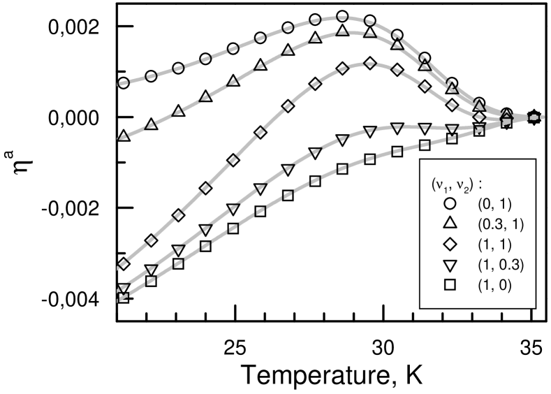
Figure 6: Relative modulation amplitude for different pairs $(\nu_{1},\nu_{2})$: solid lines are obtained with the variational method and symbols with estimate (4).

5 Conclusions

Angular and temperature dependence of the upper critical field of MgB₂ have been determined within the two-gap GL theory. We have used two different numerical methods which are in excellent agreement with each other and yield an unconventional anisotropy of $H_{c2}$ observed in the superconductor MgB₂. Such a behavior reflects the different Fermi sheet geometries and the varying importance of the small $\pi$-gap. The zeroth Landau levels employed in the variational approach are sufficient for accurate description of the continuous transition at $H_{c2}$. Contrary to the single-gap case, spatial anisotropy of the gap functions in the plane perpendicular to the magnetic field changes with temperature and can be different for each band. This explains the deviation from the effective mass angular dependence (12) applicable to ordinary superconductors. Existence of two different characteristic lengths should also affect the vortex core shape,zhitomirsky especially when an applied field is perpendicular to the $c$-axis. The gap functions have an effective single-component behavior only in a temperature region near $T_{c}$ significantly narrower than the range for the validity of the two-gap GL theory $\sim(T_{c}-T)/T_{c}\sim 1/7$. At last, the hexagonal $ab$-plane modulation of $H_{c2}$ arising from the crystal symmetry can result in a change of the sign of the hexagonal harmonics of $H_{c2}(\theta)$ when the temperature is decreased.

References

- (1) H. Suhl, B. T. Matthias, and L. R. Walker, Phys. Rev. Lett. 3, 552 (1959).
- (2) V. A. Moskalenko, Fiz. Met. Metalloved. 8, 503 (1959) [Sov. Phys. Met. Matallogr. 8, 25 (1959)].
- (3) J. Nagamatsu, N. Nakagawa, T. Muranaka, Y. Zenitani, and J. Akimitsu, Nature 410, 63 (2001).
- (4) See for review on MgB2 the special issue Physica C 385, 1-305 (2003).
- (5) M. Angst, R. Puzniak, A. Wisniewski, J. Jun, S. M. Kasakov, J. Karpinski, J. Roos, and H. Keller, Phys. Rev. Lett. 88, 167004 (2002)
- (6) L. Lyard, P. Samuely, P. Szabo, T. Klein, C. Marcenat, L. Paulius, K. H. P. Kim, C. U. Jung, H.-S. Lee, B. Kang, S. Choi, S.-I. Lee, J. Marcus, S. Blanchard, A. G. M. Jansen, U. Welp, G. Karapetrov, and W. K. Kwok, Phys. Rev. B 66, 180502 (2002).
- (7) R. Cubitt, S. Levett, S. L. Bud’ko, N. E. Anderson, and P. C. Canfield, Phys. Rev. Lett. 90, 157002 (2003).
- (8) Z. X. Shi, M. Tokunaga, T. Tamegai, Y. Takano, K. Togano, H. Kito, and H. Ihara, Phys. Rev. B 68, 104513 (2003).
- (9) A. Rydh, U. Welp, A. E. Koshelev, W. K. Kwok, G. W. Crabtree, R. Brusetti, L. Lyard, T. Klein, C. Marcenat, B. Kang, K. H. Kim, K. H. P. Kim, H.-S. Lee, and S.-I. Lee, Phys. Rev. B 70, 132503 (2004).
- (10) A. A. Golubov, A. Brinkman, O. V. Dolgov, J. Kortus, and O. Jepsen, Phys. Rev. B 66, 054524 (2002).
- (11) A. A. Golubov and A. E. Koshelev, Phys. Rev. B 68, 104503 (2003).
- (12) P. Miranovic, K. Machida, and V. G. Kogan, J. Phys. Soc. Jpn. 72, 221 (2003).
- (13) V. G. Kogan and S. L. Bud’ko, Physica C 385, 131-142 (2003).
- (14) T. Dahm and N. Schopohl, Phys. Rev. Lett. 91, 017001 (2003).
- (15) A. Gurevich, Phys. Rev. B 67, 184515 (2003).
- (16) M. Arai and T. Kita, J. Phys. Soc. Jpn. 73, 2924 (2004).
- (17) R. Cubitt, M. R. Eskildsen, C. D. Dewhurst, J. Jun, S. M. Kazakov, and J. Karpinski, Phys. Rev. Lett. 91, 047002 (2003).
- (18) M. E. Zhitomirsky and V. H. Dao, Phys. Rev. B 69, 054508 (2004).
- (19) D. R. Tilley, Proc. Phys. Soc., 84, 573 (1964).
- (20) B. T. Geilikman, R. O. Zaitsev, and V. Z. Kresin, Fiz. Tverd. Tela 9, 821 (1967) [Sov. Phys. Solid State 9, 642 (1967)].
- (21) Y. Kong, O. V. Dolgov, O. Jepsen, and O. K. Andersen, Phys. Rev. B 64, 020501 (2001).
- (22) I. I. Mazin and V. P. Antropov, Physica C 385, 49 (2003).
- (23) I. I. Mazin, O. K. Andersen, O. Jepsen, O. V. Dolgov, J. Kortus, A. A. Golubov, A. B. Kuz’menko, and D. van der Marel, Phys. Rev. Lett. 89, 107002 (2002).
- (24) S. V. Pokrovsky and V. L. Pokrovsky, Phys. Rev. B 54, 13275 (1996).
- (25) M. R. Skokan, R. C. Morris, and W. G. Moulton, Phys. Rev. B 13, 1077 (1976).
- (26) P. C. Hohenberg and N. R. Werthamer, Phys. Rev. 153, 493 (1967).
- (27) K. Takanaka, Prog. Theor. Phys. 46, 1301 (1971).