Mesoscopic threshold detectors: Telegraphing the size of a fluctuation

Abstract

We propose a two-terminal method to measure shot noise in mesoscopic systems based on an instability in the current-voltage characteristic of an on-chip detector. The microscopic noise drives the instability, which leads to random switching of the current between two values, the telegraph process. In the Gaussian regime, the shot noise power driving the instability may be extracted from the I-V curve, with the noise power as a fitting parameter. In the threshold regime, the extreme value statistics of the mesoscopic conductor can be extracted from the switching rates, which reorganize the complete information about the current statistics in an indirect way, “telegraphing” the size of a fluctuation. We propose the use of a quantum double dot as a mesoscopic threshold detector.

I Introduction

Shot noise in mesoscopic conductors,BB ; BS has attracted great interest, both theoretically and experimentally. While shot noise measurements are an important tool in experimental labs, the measurement of non-Gaussian noise presents an experimental challenge.reulet ; R Noise characteristics beyond the size of the typical fluctuation, known as full counting statistics (FCS),FCS1 ; FCS2 ; FCS3 are interesting because they bring additional information about the transport properties of the measured conductor. In particular, the extreme value statistics (EVS) can have qualitatively different behavior than typical fluctuations,nazarovJJ ; us0 ; SB and thus gives rise to new physical effects. How these rare fluctuations can be measured is one outstanding question that this paper is concerned with, and has only recently received attention.nazarovJJ ; PekolaJJ

The standard measurement method runs the current through a series of cables, filters and amplifiers before the noise is detected. While this works well for the noise power, and can be extended to the third cumulant with great effort,reulet ; R it is very hard to experimentally measure rare current fluctuations. A breakthrough in measurement technology came with on-chip detectors, which use superconducting devices, or quantum dots for a variety of functions, such as fast qubit read-outonchip ; rmp or high-frequency quantum noise measurement.noiseDD ; schoelkopf

In addition to the many advantages of going on-chip, a further possibility advanced in this paper is the use of two-terminal, rather than four-terminal measurements for low frequency noise. Four-terminal measurements are intrinsically limited by the small coupling constant between the measurement circuit and the conductor, as well as by the fact that the low-frequency noise can evade the measurement device by leakage through the bias line.pekolaexp In contrast, a two-terminal noise detector is strongly coupled, and detection is fundamentally a non-perturbative process that serves as a preamplifier of the low frequency microscopic noise.

Figure 1: The currents of the circuit elements are plotted as a function of the charge on the capacitor $Q$. The left element (NL) has a region of negative differential resistance, allowing bistability: The average current in the circuit is conserved at two stable points, $Q_{1,2}$, and one unstable point, $Q_{u}$. Inset: Noise measurement circuit. The mesoscopic conductor with parallel capacitor are connected in series with the nonlinear element.

In order to exploit the above advantages, we propose circuits with an instability as detectors of low frequency noise, as well as FCS. The considered on-chip circuit consists of a mesoscopic conductor with a parallel mesoscopic capacitor, connected in series with the nonlinear element (see Fig. 1).us0 The nonlinear element has a region of negative differential resistance, which allows bistability. The mesoscopic conductor loads the instability, so that there are two stable charge points on the capacitor, corresponding to two different currents through the circuit. In this bistable range, the shot noise occasionally causes the circuit to transit from one stable state to the other, producing a random telegraph signal.machlup The rate of transition is exponentially sensitive to the size of the fluctuation,us0 and thus serves as a threshold detector for the rare current fluctuations. Although the threshold rates are not a direct measurement of the FCS, they reorganize the complete information about the noise statistics in an indirect way, “telegraphing” the size of a fluctuation. Therefore, bistable systems are a promising candidate for low-frequency noise detectors, and can confirm or falsify a given prediction for FCS.

The paper is organized as follows. In Sec. II we first review the statistical properties of the general telegraph process, as well as the instanton dynamics for noise driven circuits, and the results for the bistable switching rates. This sets the stage for the application of this physical process. The implications of the Gaussian noise limit are considered in Sec. III, and we find that the I-V curve may be used to extract the noise power as a fitting parameter. The results for the second and third cumulant are also given, and the role of the asymmetry in the rates is discussed. In Sec. IV, we examine several effects that arise when the bistable circuit is combined with an external circuit. The threshold detector of EVS is introduced in Sec. V. We give results for the threshold rates of several processes, and discuss stabilization effects that arise when the tails of the distribution have a cut-off. The quantum double dot is proposed as an implementation of the threshold detector in Sec. VI. We discuss the mesoscopic circuit, needed conditions and constraints, as well as feasibility. Sec. VII contains our conclusions.

II Set-up and bistability results

We first review the essential results on the transport statistics of bistable systems.us0 Consider the circuit shown in the inset of Fig. 1, biased with voltage $V$. The average current through both circuit elements is plotted in Fig. 1 versus the charge on the parallel capacitor $C$ (we choose to speak about the charge on the capacitor, rather than the voltage across the right element $Q/C$.) The nonlinear element on the left has a range of negative differential resistance, which leads to the possibility of three charge/current points, $(Q_{1},I_{1}),(Q_{2},I_{2}),(Q_{u},I_{u})$, where the I-Q curves intersect, so the average current is conserved in the circuit. The central intersection at $Q_{u}$ is unstable to small charge perturbations, while the outer two intersections $Q_{1,2}$ are stable. The microscopic non-equilibrium noise is correlated on a short time scale $\tau_{0}\sim\hbar/eV$, and drives the collective system on the longer RC-time of the circuit, $\tau_{C}\gg\tau_{0}$. Occasionally, the microscopic noise causes the system to transit between stable states. As a result, the measured current switches back and forth between $I_{1}$ and $I_{2}$, with rates $\Gamma_{1,2}$. These rates contain valuable information about the statistical nature of the driving noise that will be examined later. On a long time scale, the system relaxes with the rate $\Gamma_{S}=\Gamma_{1}+\Gamma_{2}$ to the stationary state. This stationary state has constant probabilities to occupy one of the two stable points,

$$P_{1}=\Gamma_{2}/\Gamma_{S},\quad P_{2}=\Gamma_{1}/\Gamma_{S}.$$ (1)

Therefore, the average current is

$$\langle I\rangle=\sum_{n=1,2}I_{n}P_{n}.$$ (2)

The randomness of the duration in either of the stable states leads to the fluctuation of the transmitted charge

$${\cal Q}(t)=\int_{0}^{t}dt^{\prime}I(t^{\prime}).$$ (3)

This random variable has a probability distribution $P({\cal Q}(t))$, which may be specified by its moments. In the stationary limit, it is more convenient to consider the cumulants (irreducible correlators) because they are linear in time, $\langle\langle{\cal Q}^{n}\rangle\rangle\equiv t\langle\langle I^{n}\rangle\rangle$, and may be used to define time-independent current cumulants, $\langle\langle I^{n}\rangle\rangle$. The second cumulant and third cumulant of the switching current described above are given respectively byus0

$$\langle\langle I^{2}\rangle\rangle = \sum_{n=1,2}F_{n}P_{n}+2(\Delta I)^{2}\Gamma_{1}\Gamma_{2}/\Gamma_{S}^{3},$$ (4)

$$\langle\langle I^{3}\rangle\rangle = \sum_{n=1,2}L_{n}P_{n}+6(\Delta I)^{3}\Gamma_{1}\Gamma_{2}\Delta\Gamma/\Gamma_{S}^{5},$$ (5)

where $\Delta I=I_{2}-I_{1}$, while $F_{n}$ and $L_{n}$ are the noise power and third cumulant of the stable points, which describe the small fluctuations around $I_{1,2}$. The first term in Eq. (4) is the weighted noise power of the stationary states, and the second term is the well-known result for zero-frequency telegraph noise. machlup The telegraph contribution dominates the bare contribution because it scales as $\Gamma_{S}^{-1}$ in the second cumulant, and as $\Gamma_{S}^{-2}$ in the third.us0

An important feature of bistable systems is that the I-V curve makes a rapid transition from $I_{1}$ to $I_{2}$ as a function of the bias voltage (see Fig. 2 and the discussion below), while the current cumulants show a peak structure. During this transition, the specific values of the currents $I_{1,2}$ may be considered constant. If one has access to the first three cumulants of an unknown process, one may utilize these cumulants, Eqs. (2,4,5), to diagnose whether bistability exists or not. The dominant telegraph contribution to Eqs. (2,4) may be used to eliminate the rates, and substitution into Eq. (5) then yields the third cumulant of the telegraph process in terms of the first two:note1

$$\langle\langle I^{3}\rangle\rangle_{tel}=3\langle\langle I^{2}\rangle\rangle_{tel}^{2}\frac{(I_{1}+I_{2})/2-I}{(I_{2}-I)(I-I_{1})}.$$ (6)

This equation may serve as a valuable test of experimental data because there is no fitting parameter. The above procedure was used by Flindt, Novotny, and Jauho to demonstrate bistability in numerical studies of the nanomechanical shuttle.shuttle

The above results (2,4-6) are general and apply to any telegraph process, independent of its microscopic origin. We now turn to the bistable circuit driven by current noise. The microscopic current fluctuations $\tilde{I}_{L,R}$ of the two circuit elements may be described with generating functions of the current cumulants (that are Markovian after the correlation time $\tau_{0}$),

$$H_{\alpha}(\lambda_{\alpha})=\sum_{n}(\lambda_{\alpha}^{n}/n!)\langle\langle{\tilde{I}}^{n}_{\alpha}\rangle\rangle,\quad\alpha=L,R,$$ (7)

where the cumulants $\langle\langle{\tilde{I}}^{n}_{\alpha}\rangle\rangle$ are functions of the charge on the capacitor $Q$ (we set the electron charge e=1 throughout the paper). The fact that the correlation time $\tau_{0}$ is much smaller than the RC-time $\tau_{C}$ of the circuit, means the slow dynamics is classical.us1 The circuit dynamics may now be described with the stochastic path integral formalism.us1 ; us2 This formalism is quite general and has been applied to a wide variety of stochastic problems in mesoscopic physics.SB ; us0 ; spi1 ; spi2 ; spi3 ; spi4 In addition to the separation of time scales, we require that the instability is well developed, so that the stochastic bistable switching rates are given byus0

$$\Gamma_{1,2}=\omega_{1,2}\exp(-A_{1,2}),$$ (8)

where the action

$$A_{1,2}=\int^{Q_{u}}_{Q_{1,2}}dQ\,\lambda_{\rm in}(Q),$$ (9)

must be larger than one. The attempt frequency $\omega_{1,2}$ is subdominant and will be neglected. The function $\lambda_{\rm in}(Q)$ (which we refer to as the instanton line) is implicitly defined by the nontrivial solution of the algebraic equationus0

$$H(Q,\lambda)=H_{L}(Q,\lambda)+H_{R}(Q,-\lambda)=0,$$ (10)

which can be found for arbitrary noise statistics by a reversion of the power series,

$$H(\lambda)=(I_{L}-I_{R})\lambda+(1/2)(F_{L}+F_{R})\lambda^{2}+\ldots=0,$$ (11)

where $I_{L,R}\equiv\langle\tilde{I}_{L,R}\rangle$ and $F_{L,R}\equiv\langle\langle\tilde{I}^{2}_{L,R}\rangle\rangle$.

There are two physical limits that we now consider, based on the comparison of the maximum current difference through the instability $\delta I={\rm max}\{|I_{L}-I_{R}|\}$ (referred to as the current threshold) to the total noise power at the instability, $F=(F_{L}+F_{R})$. In the Gaussian limit, discussed in the next section, the current threshold is small compared to the total noise power, $\delta I\ll F$ so the system is effectively driven by Gaussian noise alone, with higher current cumulants making only small corrections. In the threshold limit, discussed in Sec. V, the current threshold is large compared to the total noise power, $\delta I>F$, so it will be the tails of the distribution that drive the switch.

In the counting statistics literature, it is usually the generating function of the stochastic process that is sought. We would like to comment that the instanton line (10) for a noiseless nonlinear element characterizes the stochastic process in a different way that nevertheless contains all the information about the rare events. Furthermore, it is directly related to a physical quantity that is readily observed in experiments, the switching rate (8), and therefore provides a more useful characterization of the EVS.

III I-V curve in the Gaussian limit

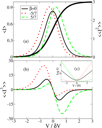
Figure 2: (color online). The average current $\langle I\rangle$, the noise $\langle\langle I^{2}\rangle\rangle$, and third cumulant $\langle\langle I^{3}\rangle\rangle$ are plotted as a function of the scaled voltage, for different asymmetry parameters, $\beta$. (a) The asymmetry is invisible in the current, but it produces a shift in the peak location of the noise. (b) The asymmetry is further magnified in the third cumulant, that shows a weighted peak and dip. (c) By plotting the logarithm of the ratio ${\cal G}=(dI/dV)/\langle\langle I^{2}\rangle\rangle$ versus voltage, the asymmetry parameter $\beta$ is given asymptotically by the negative difference of the slopes, divided by the sum of the slopes. We have taken $I_{1}=0,I_{2}=1$, $V_{0}=0$, and $\Gamma_{0}=.1$.

We now consider the Gaussian limit, $\delta I\ll F$, and demonstrate how to extract the noise alone from the telegraph process. Keeping only the first two terms in Eq. (11), the instanton line is given by

$$\lambda_{\rm in}(Q)=-2(I_{L}-I_{R})/(F_{L}+F_{R}),$$ (12)

implying that $|\lambda_{\rm in}|\ll 1$ and justifying the series truncation. To leading order in $\delta I/F$, the microscopic noise is constant, $F=F_{L}+F_{R}=const$, and may be taken out of the action integral. For a well developed instability, $A_{1,2}>1$, the current will make a transition from $I_{1}$ to $I_{2}$ on a voltage scale smaller than the total instability scale $(Q_{2}-Q_{1})/C$ (see below). On this smaller voltage scale, the currents $I_{1,2}$ are approximately constant, and we may linearize the actions $A_{1,2}$ in voltage around the point $V_{0}$ where they are equal, $A_{1}=A_{2}$. This linearization gives the transition rates,

$$\Gamma_{1,2}=\Gamma_{0}\exp[-(2C/F)(I_{1,2}-I_{u})(V-V_{0})],$$ (13)

where $I_{1,2}$ and $I_{u}$ are taken at $V=V_{0}$. The rates have an activation form with (in general) different energy scales. Nevertheless, the I-V curve, Eq. (2), depends only on the ratio of the rates, and therefore has a universal form,

$$I(V)=\frac{I_{1}+I_{2}}{2}+\frac{\Delta I}{2}\tanh\left[(C\,\Delta I/F)\,(V-V_{0})\right].$$ (14)

Thus, as a function of $V$, the current has a step on a voltage scale $\delta V=F/(C\Delta I)$. The conditions $A_{1,2}\sim|Q_{1,2}-Q_{u}|\delta I/F>1$ and $\Delta I>\delta I$, imply $\delta V<(Q_{2}-Q_{1})/C$, so the action linearization is justified.

Assuming the capacitance $C$ is known, the noise power driving the instability can be accurately obtained by fitting data with Eq. (14), with $F$ as the only fitting parameter. In contrast, the noise power and third cumulant of the telegraph process do not have a universal form because they depend on the rates directly. The behavior of the cumulants may be characterized by an asymmetry parameter $\beta=(I_{1}+I_{2}-2I_{u})/\Delta I$ that describes the difference in the activation energy scales of the rates (13). In Fig. 2, we plot the first three cumulants, Eq. (2,4,5), for the rates in Eq. (13) versus the normalized external voltage for different values of the asymmetry parameter. The asymmetry is invisible in the current, creates a small shift in the noise peak, and is further magnified in the third cumulant. We would like to stress that the third cumulant may have either a peak or dip, depending on the sign of the asymmetry parameter. The asymmetry may be directly extracted by plotting the logarithm of the ratio ${\cal G}=(dI/dV)/\langle\langle I^{2}\rangle\rangle$ versus bias and reading off the asymptotic slope as done in Fig. 2c. The asymmetry parameter $\beta$ is given by the negative difference of the slopes, divided by the sum of the slopes.

By first calibrating with an equivalent resistor to determine $F_{L}$ and $C$, (where the bistable system is driven by the noise of the nonlinear system alone), the shot noise power $F_{R}$ of the mesoscopic sample may be extracted. Alternatively, one may use a nonlinear system with known noise properties. Note also, that the detailed shape of the nonlinear I-V is not important, so long as the above assumptions are met. The accuracy of the measurement is limited by the accuracy of the I-V curve. The signal-to-noise ratio grows as the square root of the number of switches, and should be large. To move to another bias point, the nonlinear I-V curve should be shifted up. This can be done by attaching an additional current bias line between the circuit elements, e.g. with a separate bias and tunnel junction. The external voltage and current bias allow a fully tunable bistability. This method may be applied even for macroscopic unstable systems, such as resonant tunneling diodes, rtw1 ; rtw2 ; rtw3 because while $C$ is large, $\delta I$ can always be made smaller by shifting the bias to reduce the current barrier.

IV External circuit effects

In this section, we investigate how the external circuit can influence the statistical properties of the bistable system. In the first experiment on non-Gaussian noise, feedback effects from the external circuit played an important role.reulet ; beenakker If the mesoscopic system is imperfectly voltage biased, the voltage across the mesoscopic sample will fluctuate on a long time scale. These slow fluctuations alter the transport conditions, and provide additional contributions to the individual current cumulants, named ‘cascade corrections’.Nagaev1 ; Nagaev2 ; us2 We argue below that the voltage fluctuations across the circuit may also affect the switching rates.

We begin this analysis by considering a common experimental set-up, the current biased circuit, where the external circuit resistance is much larger than the sample resistance. The large circuit resistor fixes the current through the sample so current fluctuations vanish, creating voltage fluctuations instead. The transport dynamics is characterized by three relevant time scales. The RC time of the system $\tau_{C}$, the RC time of the external circuit $\tau_{RC}$, and the inverse switching rate $\Gamma_{S}^{-1}$.

Figure 3: System dynamics in the case of a current biased circuit. Starting at $V_{1}$, the system can hop to the empty circle at $V_{u}^{(1)}$ on the time scale $\tau_{C}$, and then fall to the black dot on the lower dashed load line. This creates a current below the external current bias, so the circuit adiabatically adjusts by moving along the arrow to $V_{2}$ on the time scale $\tau_{RC}$. After a time on the order of $\Gamma_{S}^{-1}$, the system can then hop over the barrier to the empty circle at voltage $V_{u}^{(2)}$, and fall to the black dot on the upper dashed load line. This state has a current above the bias current, so the system adiabatically follows the arrow back down to $V_{1}$ on the time scale $\tau_{RC}$, completing the cycle.

Any realistic measurement circuit is current biased on the external RC-time, longer than the system relaxation time, leading to the ordering,

$$\tau_{C}\ll\tau_{RC},\Gamma_{S}^{-1}.$$ (15)

We first consider the experimental situation when the typical time spent in the stable states is much longer than the external circuit RC-time,

$$\tau_{RC}\ll\Gamma_{S}^{-1}.$$ (16)

In this parameter range, the dynamics is sketched in Fig. 3. On the time scale $\tau_{C}$, the average voltage across the nonlinear system changes very little, so the dynamics is effectively voltage biased. The system transitions from $V_{1}$ or $V_{2}$ to the black dot along the slanted load line. On the time scale $\tau_{RC}$, the voltage across the nonlinear element adiabatically relaxes to restore the current to its proper value. The system then switches again on the other slanted line after a time $\Gamma_{S}^{-1}$. The main difference with respect to the voltage biased case is that the step will be in voltage, not current, and therefore the I-V curve will have a plateau, not a step. Repeating the derivation that lead to Eq. (14), we find,

$$V(I)=\frac{V_{1}+V_{2}}{2}+\frac{\Delta V}{2}\tanh\left[(C{\widetilde{\Delta V}}/F)\,(I-I_{0})\right],$$ (17)

where $I_{0}$ is the current value where the rates are equal, and ${\widetilde{\Delta V}}=\Delta V+V^{(1)}_{u}-V^{(2)}_{u}$ is not the same as in the prefactor because the values of the unstable voltage are different in the shifted curves of Fig. 3. This non-universality will be small if the mesoscopic element has a large resistance, so $V^{(1)}_{u}-V^{(2)}_{u}$ is small. As the above analysis shows, the usual experimental procedure of taking voltage noise data, and converting it into current noise fails if there is an instability.

A separate circuit effect arises because the stable current state produces its own shot noise, that the external resistor suppresses, creating voltage noise on a time scale $\tau_{RC}$ across the mesoscopic part of the circuit. This voltage noise adiabatically rocks the current threshold, increasing the average transition rate. The relative magnitude of this effect can be estimated by comparing the variance of the rocking potential with the voltage scale of the transition, $\delta V$, and is small if $\tau_{C}\ll\tau_{RC}$, as we have assumed.

Considering now the regime

$$\Gamma_{S}^{-1}\ll\tau_{RC},$$ (18)

where the telegraph switching is fast compared to the external circuit response time, we see that the voltage across the sample has no time to change until after the next switching event restores the current to its original value. In this regime, the switching is always voltage biased. Furthermore, we may consider the whole sample as a fast Langevin noise source with telegraph current statistics that drives the charge fluctuations in the external circuit. Current cumulants may now be computed in the usual way for stable systems with a nonlinearity.us2 ; note3

V Threshold Detectors and Full Counting Statistics

Figure 4: Schematic of the average current flowing through the threshold detector and Ohmic mesoscopic conductor as a function of the charge. The detector current has a peak with center $Q_{0}$, width $\Delta Q$, and maximum current $I_{0}$. The mesoscopic conductor is defined to have currents $I=I_{m}$ and $I=0$ at the stable states.

We now propose a measurement scheme for the EVS of a mesoscopic conductor. The idea is to use the bistable system as threshold detector, in the limit $\delta I>F$, where the switch will be driven by the non-Gaussian tails of the current distribution. We consider the shot noise regime, where the current cumulants are proportional to the average current, $H_{\alpha}(Q,\lambda)=I_{\alpha}(Q)h_{\alpha}(\lambda)$, and $h_{\alpha}$ generates the generalized Fano factors. Then, Eq. (10) for the instanton line takes the following form,

$$-h_{L}(\lambda)/h_{R}(-\lambda)=I_{R}(Q)/I_{L}(Q)\equiv{\cal R}(Q).$$ (19)

In this equation, all the non-universal details of the charge dependence of the instability appear on the rhs in the current ratio ${\cal R}$, while the statistical nature of the fluctuations appears on the lhs. In order to probe the probability of having a very large (small) current in the mesoscopic system, the threshold limit we are now concerned with implies that the extremal value of ${\cal R}$ through the instability is much smaller (larger) than 1. This means that in contrast to the Gaussian limit, where Eq. (19) gives $\lambda_{m}\equiv{\rm max}\{|\lambda_{\rm in}|\}\ll 1$, the threshold limit implies $\lambda_{m}>1$. This corresponds to large action, or a very small switching rate, which makes the measurement of the FCS experimentally challenging. To overcome this difficulty a general strategy should be based on the following ingredients:

1. A separation of time scales, that allows the measurement of the Markovian FCS of the fast microscopic noise sources that drive the classical circuit on a longer time scale.

2. The action $A\sim\Delta Q\lambda_{m}$ must be larger than one, but not so large that the system never switches on experimental time scales.

3. The instability must be such that the current ratio ${\cal R}=I_{R}/I_{L}$ is larger (or smaller) than one in the bistable range, so that $\lambda_{m}\geq 1$.

4. A sufficiently large bias, so that the circuit is both in the bistable range, and the bias across the mesoscopic element exceeds the temperature.

5. A further useful (but not essential) ingredient is that the nonlinear element is noiseless, so that the transition is driven by the mesoscopic element alone.

Condition (2) is the most severe constraint. In order to have the action not too large, $\Delta Q$ must be comparable to the electron charge, implying that the capacitance of the circuit is in the mesoscopic range. This excludes macroscopic nonlinear elements such as tunnel diodes from measuring full counting statistics (though not Gaussian noise, see Sec. III). Conditions (2) and (3) together determine the necessary shape of the instability. In order to have $\Delta Q$ small, and ${\cal R}=I_{R}/I_{L}$ large, the I-Q characteristic of the nonlinear element should have a sharp peak or dip, the first of which is shown in Fig. 4.

To measure FCS using this peak, the switching rate should be measured as a function of the external bias, that moves the mesoscopic load line down the peak. This procedure is sketched in the inset of Fig. 5, which shows the real time switching from the stable point with average current $I_{m}$, via the current peak, to the other stable point with zero current. The dependence of $I_{m}$ versus $V-V_{th}$ is shown in Fig. 5, where $V_{th}$ is the value of the external bias at the current maximum. A direct measure of the current EVS may be obtained by dividing the log-rate by the voltage jump, in order to remove the effect of the shape of the current peak, and plotting

$$S=(\log\Gamma)/C(V-V_{th}),$$ (20)

versus $I_{m}/I_{0}$.

Figure 5: Sketch of the experimental procedure to extract the EVS of a mesoscopic conductor. The current in the conductive state $I_{m}$ decays as a function of the external bias on the scale of the peak width $\gamma$. Inset: The system will switch from the conducting state to the insulating state on a time scale $1/\Gamma_{2}$

We now consider the switching rate for Poissonian, Gaussian, and Binomial noise sources while assuming a noiseless nonlinear element ($h_{L}=\lambda$) so that the switching dynamics is governed solely by the system noise. The characterization of EVS can be extracted from the divergence of the action, which corresponds to large values of $\lambda_{m}$. We compare the most important processes: Gaussian, $h_{R}(\lambda)=\lambda+\lambda^{2}/2$ (Fano factor is 1); Poissonian, $h_{R}(\lambda)=\exp\lambda-1$; and Binomial, $h_{R}(\lambda)=T^{-1}\log[1+T(\exp\lambda-1)]$. In the asymptotic limit ($|\lambda|\rightarrow\infty$), Eq. (19) may be solved to obtain:

$$\lambda_{\rm in}=\begin{cases}-1/{\cal R},&{\rm Gaussian}\cr\log{\cal R},&{\rm Poissonian}\cr(T\log T)/({\cal R}-T),&{\rm Binomial}\end{cases}$$ (21)

which replaces Eq. (12).

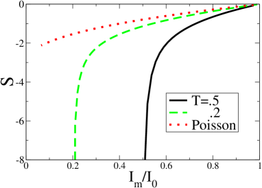
Figure 6: (color online). The normalized log-rate $S$ is plotted versus $I_{m}/I_{0}$ for a quantum point contact with transparencies $T=.5$ and $T=.2$ measured by a noiseless detector with current peak of Lorentzian shape. $S$ has a power-law divergence as $I_{m}/I_{0}$ approaches $T$, which is a manifestation of the ‘Pauli stabilization’ effect (see text). Comparison is also shown with the Poissonian limit, whose divergence at the origin is cut off by the finite conductance of the QPC.

It is important that all three processes have very different asymptotic behaviors that makes it relatively easy to distinguish them in experiments. However, the most surprising fact is that the Binomial process, characteristic of a quantum point contact with transparency $T$, has a sharp power-law singularity at ${\cal R}=T$. It persists even at small $T$ (the tunneling limit) which is usually considered to give a Poissonian process. This behavior (discussed previously by Tobiska and Nazarov in Ref. nazarovJJ, ) has the following physical interpretation: The total charge that passes the conductor is the sum of independent electron attempts, with success probability $T$, and failure probability $1-T$. The Pauli principle allows only one electron at a time to make an attempt. Therefore, the current distribution has a sharp cut-off at the maximum allowed current, when all attempts are successful. This maximum current is given by $I_{max}=\langle I\rangle/T$. If the current threshold ratio $\cal R$ is lowered below $T$, the mesoscopic conductor has no chance to have a large enough fluctuation to overcome the barrier, and the system never switches. We propose the name “Pauli stabilization” to describe this impotency. To further illustrate the effect, we plot $S$ Eq. (20) for a Lorentzian peak in Fig. 6, using a quantum point contact with different transparencies. Even if the transparency is fairly small, where Poissonian statistics is naively expected, there is still a power-law divergence in $S$. This divergence may be estimated by expanding ${\cal R}\approx{\cal R}_{0}+\alpha Q^{2}$ near the peak, to obtain

$$S\sim-(T\log T)/\sqrt{\alpha({\cal R}_{0}-T)}.$$ (22)

An interesting situation occurs when the bistable system is driven by a microscopic noise that is itself a random telegraph process. For instance, a charge trap near the right mesoscopic conductor may switch the current between $I_{a}$ and $I_{b}$, with rates $\Gamma_{a,b}$. The generating function of this random process isus0

$$H_{R} = \frac{1}{2}(I_{a}+I_{b})\lambda-\frac{1}{2}(\Gamma_{a}+\Gamma_{b})$$ (23)

$$+ \sqrt{[(I_{b}-I_{a})\lambda-\Gamma_{b}+\Gamma_{a}]^{2}/4+\Gamma_{a}\Gamma_{b}}.$$

The instanton line (10) has an exact solution for a noiseless nonlinear element,

$$\lambda_{\rm in}(Q)=\frac{\Gamma_{a}}{I_{L}-I_{a}}+\frac{\Gamma_{b}}{I_{L}-I_{b}}.$$ (24)

An important check is $\lambda_{\rm in}=0$ when $I_{L}=I_{R}=(\Gamma_{b}I_{a}+\Gamma_{a}I_{b})/(\Gamma_{a}+\Gamma_{b})$. On the other hand, the instanton solution diverges when $I_{L}$ approaches $I_{a}$ or $I_{b}$, where the distribution has a cut-off,us0 and thus also displays a stabilization effect. As $I_{L}$ approaches $I_{a}$ or $I_{b}$, the currents may be approximated as $I_{b}-I_{L}\approx(I_{b}^{0}-I_{L}^{0})+\epsilon\,Q^{2}$, so the action itself has a power-law divergence as

$$S\sim-\Gamma_{a,b}/\sqrt{\epsilon\,(I_{b}^{0}-I_{L}^{0})}.$$ (25)

It is important to note that because the telegraph process has a much larger noise power than shot noise, this stabilization effect should be able to be observed even with macroscopic nonlinearities, such as tunnel diodes. To see why this is so, we estimate the action away from the divergence as $S\sim\Gamma_{a,b}\,\tau_{C}$. Our time scale separation demands that $\Gamma_{a,b}>\tau_{C}$, so $S>1$. Other than this requirement, $\Gamma_{a,b}$ is an independent parameter. Therefore, the action can be made of order one even with a large capacitance, so the action divergence from the EVS stabilization behavior in Eqs. (24,25) should be able to be seen on experimental time scales.

VI Double quantum dot as a threshold detector

While the discussion has thus far been rather general, we now concentrate on a specific implementation of the mesoscopic threshold detector, a quantum double dot (DD).DDreview We consider the resonant tunneling regime, where each dot has a Breit-Wigner resonance of Lorentzian shape.stone ; markus The transmission as a function of energy is

$$T(E)=\frac{4\gamma^{2}t^{2}}{|(E-E_{0}+i\gamma)(E+E_{0}+i\gamma)|^{2}},$$ (26)

where $\gamma$ is the total decay width of the symmetric resonant levels, $t$ is the tunnel coupling of the middle barrier, $E_{0}^{2}=t^{2}+(\Delta E)^{2}/4$ is the hybridized energy of the levels, and $\Delta E$ is the energy difference between the levels that can be adjusted with gate voltages. The total current through the double dot also has a Lorentzian shape as a function of $\Delta E$,

$$I=\frac{2\pi\gamma t^{2}}{\gamma^{2}+E_{0}^{2}},$$ (27)

and is maximal at $I_{\rm max}=\pi\gamma$ for $\gamma=t$, and $\Delta E=0$. Despite the fact that the transparencies of the barriers are low, the total current is large in the resonant tunneling limit. In Fig. 4, $\Delta E\propto Q$, where the coefficient is relative capacitance of the two levels to the cavity, and $\Delta Q\propto\gamma$. The Fano factor $f$ at $\Delta E=0$ as a function of the dimensionless ratio $r$ is

$$f=\frac{2r^{4}-r^{2}+1}{2(1+r^{2})^{2}},\quad r=\gamma/t,$$ (28)

and has a minimum at $r=\sqrt{3/5}$, where the Fano factor is $f_{\min}=7/32\approx.219$. At this point, the noise is suppressed, but not zero. It is well known that a single Breit-Wigner resonance has a Fano factor of $1/2$, and here with a double-dot, it is suppressed below $1/4$. These results naturally lead to the idea that a series of quantum dots, or a ballistic narrow-band conductor, may be used as an ideal noise detector.

This double dot is fabricated together with a quantum point contact (QPC) connected through a mesoscopic cavity as sketched in Fig. 7. The physics of the switch is as follows. Current is flowing through the DD with the right level slightly above the left, and flowing out the QPC. The QPC has a rare event, where many subsequent electrons succeed in exiting the right contact. This depresses the charge in the cavity below the average, lowering the potential on the cavity. The potential capacitively couples asymmetrically to the two quantum dots which aligns the levels on the DD, producing more current flowing into the cavity. The QPC continues in its rare event, further lowering the potential in the cavity, finally misaligning the levels to the unstable point, and cutting off transport.

Figure 7: A double quantum dot in series with a mesoscopic quantum point contact with transmission $T_{M}$. A metallic side gate provides a tunable capacitance.

We now make some estimates of the energy scales and parameter ranges for the circuit to function as we wish. There should only be a few resonant levels in the transport window, so the typical energy spacing between the adjacent peaks in the I-V curve will be the mean level spacing of the quantum dots, $\Delta_{D}$. The width of the current peak is $\gamma<\Delta_{D}$, implying the peaks are separated. The current at the top of the peak is given by the peak conductance times the width of the barrier, $I_{0}\leq\gamma$, where equality is reached in the perfect resonant tunneling limit.

The first condition is on the conductance of the mesoscopic sample $T_{M}$ (we set the conductance quantum equal to 1), so the load line crosses one peak only, as shown in Fig. 4,

$$I_{0}/\gamma>T_{M}>I_{0}/\Delta_{D}.$$ (29)

The left inequality is most strict for an open QPC, which requires perfect resonant tunneling. The right inequality is not very restrictive, since $I_{0}/\Delta_{D}=(I_{0}/\gamma)(\gamma/\Delta_{D})<1$, which allows the pinch-off limit.

The next condition is the time scale separation between the RC-time of the cavity, and the tunneling time through the DD. In the case, $C>\Delta_{C}^{-1}$, where $C$ is the geometrical capacitance, and $\Delta_{C}$ is the mean level spacing in the connecting cavity at the Fermi energy, $C_{\mu}^{-1}=(C^{-1}+\Delta_{C})\approx\Delta_{C}$. The time scale separation condition $\gamma>\Delta_{C}T_{M}$, simply means that the cavity is larger than the quantum dots. Additionally, the action must not be too large, so for the FCS measurement (where $\lambda_{m}>1$), the charge difference, $\Delta Q$, must not be too large. The charge width is given by the density of states of the cavity, times the peak’s voltage width, $\Delta Q\sim\gamma/\Delta_{C}$. Together, these two conditions constrain the size of the cavity,

$$\gamma/T_{M}>\Delta_{C}>\gamma/\Delta Q,$$ (30)

which gives a rather small parameter range.

Finally, to go out of equilibrium, the system must be cooled to mesoscopic temperatures, $T<I_{0}/T_{M}$, much smaller than the mean level spacing of the small quantum dot. However, it would be also interesting to observe EVS even in equilibrium. While the noise power in equilibrium is simply a consequence of the fluctuation-dissipation theorem, the EVS is nontrivial.

We now compare our idea with other proposals for measuring noise and EVS of mesoscopic conductors. In the proposals discussed below, the measurement device is in a separate circuit weakly coupled to the mesoscopic conductor that acts as an external noise source. Aguado and Kouwenhoven proposed a double quantum dot as a detector of high frequency noise.noiseDD The quantum noise causes inelastic transitions between the states of quantum dot, and therefore the double dot current is proportional to the noise power at that frequency. Tobiska and Nazarov proposed using Josephson junctions as a measurement device.nazarovJJ A rare current fluctuation causes the quantum phase to jump over the top of its effective potential, creating a transition from the superconducting phase to the normal conducting phase. The switching rate gives information about the probability of the rare current fluctuation. Macroscopic quantum tunneling is suppressed by having an array of Josephson junctions to make the potential barrier width large. Pekola also proposed using Josephson junctions as a measurement device.PekolaJJ In this proposal, the noise first creates a transition from the ground state to the first excited state, where macroscopic quantum tunneling causes escape.

The noise experiment implementing this last proposal, Ref. [pekolaexp, ], provided additional clarification of the difficulties involved in measuring FCS. Similarly to the double-dot detector, noiseDD the Josephson junction measured noise at the plasma frequency of the junction, while the low frequency noise leaked through the bias line. This also explained why the expected exponential dependence of the rate on the current threshold was not found.

Our proposal is based on essentially different physics: The threshold detector is supposed to work in a regime where detection is a non-perturbative process due to strong coupling to the measured system. Although a realization of this threshold detector is an experimental challenge, there are several advantages of our proposal. The separation of time scales requirement $\tau_{C}\gg\tau_{0}$ is necessary to measure low frequency noise: The finite response time allows many electrons to enter and leave the cavity, so the Markovian limit is reached. This limit also implies that quantum effects are not relevant. Detector feedback, usually a liability, is completely accounted for. In fact, detector feedback is an essential ingredient for our proposal.

VII Conclusions

We have proposed the use of circuit instabilities as two-terminal detectors of low-frequency noise. The considered circuit consists of a mesoscopic conductor with parallel capacitor, in series with a nonlinear element. The nonlinear device contains a region of negative differential resistance, which allows bistability. There are two regimes of interest, from the point of view of shot noise measurement.

The first is the Gaussian regime, where the noise power is much larger than the current threshold. In this limit, the noise power is effectively constant, and the higher cumulants may be neglected. The noise drives a transition between two current values, the telegraph process. This process produces a step in the I-V curve of universal form, with only one variable parameter, from which the noise power may be extracted. The second cumulant has a peak at the current step, while the third cumulant has a peak and a dip, the relative weight depending on an asymmetry parameter of the switching rates. We further considered external circuit effects. In the current biased case, the dominant effect is that the I-V curve has a plateau, not a step, because it is the voltage that switches, not the current. The measurement of Gaussian noise may be carried out with macroscopic conductors containing nonlinearities, such as resonant tunneling wells.

The second regime is the threshold regime, where the noise power is smaller than the current threshold. In this limit, the switch comes from the tails of the distribution, and is a direct signature of the extreme value statistics of the mesoscopic conductor. The most interesting effect occurs for charge distributions that have a cut-off. This cut-off manifests itself in a divergence of the switching rate, that stabilizes the state. We considered both Pauli stabilization from a quantum point contact, as well as stabilization from a microscopic random telegraph process. While the measurement of full counting statistics requires a mesoscopic instability because of the long time scales involved, the stabilization effect from the random telegraph process should be visible in macroscopic nonlinear elements. We proposed a quantum double dot operating in the resonant tunneling regime as an implementation of the threshold detector of rare shot noise fluctuations. Constrains on the conductance of the measured conductor, and the capacitance of the central dot were discussed.

- (1) Ya. M. Blanter and M. Büttiker, Physics Reports 336, 1 (2000).
- (2) C.W.J. Beenakker and C. Schönenberger, Physics Today, 56, 37 (2003).
- (3) B. Reulet, J. Senzier, and D. E. Prober, Phys. Rev. Lett. 91, 196601 (2003).
- (4) M. Reznikov et al., unpublished experiment.
- (5) L. S. Levitov and G. B. Lesovik, Pis’ma Zh. Eksp. Teor. Fiz. 58, 225 (1993).
- (6) L. S. Levitov, H. Lee and G. B. Lesovik, J. Math. Phys. 37, 4845 (1996).
- (7) Quantum Noise in Mesoscopic Systems, edited by Yu. V. Nazarov NATO Science Series II Vol. 97 (Kluwer, Dordrecht, 2003).
- (8) J. Tobiska and Yu. V. Nazarov, Phys. Rev. Lett. 93, 106801 (2004).
- (9) A. N. Jordan and E. V. Sukhorukov, Phys. Rev. Lett. 93, 260604 (2004).
- (10) E. V. Sukhorukov and O. M. Bulashenko, Phys. Rev. Lett. 94, 116803 (2005).
- (11) J. P. Pekola, Phys. Rev. Lett. 93, 206601 (2004).
- (12) Y. Nakamura, Yu. A. Pashkin, and J. S. Tsai, Nature (London), 398, 786 (1999).
- (13) Y. Makhlin, G. Schön, and A. Shnirman, Rev. Mod. Phys. 73, 357 (2001).
- (14) R. Aguado and L. P. Kouwenhoven, Phys. Rev. Lett. 84, 1986 (2000).
- (15) R. J. Schoelkopf, A. A. Clerk, S. M. Girvin, K. W. Lehnert, and M. H. Devoret, in Ref.FCS3, .
- (16) J.P. Pekola, T.E. Nieminen, M. Meschke, J.M. Kivioja, A.O. Niskanen, J.J. Vartiainen, cond-mat/0502446.
- (17) S. Machlup, J. Appl. Phys. 25, 341 (1954).
- (18) If the rates are not that small, it is important to first subtract off the noise background in Eqs. (4,5) before applying the self-consistent check. This is straightforward to do, because the crossover between the stable states in higher order cumulants is also universal.
- (19) C. Flindt, T. Novotny, and A.-P. Jauho, Europhys. Lett., 69, 475 (2005).
- (20) S. Pilgram, A. N. Jordan, E. V. Sukhorukov, and M. Büttiker, Phys. Rev. Lett. 90, 206801 (2003).
- (21) A. N. Jordan, E. V. Sukhorukov, and S. Pilgram, J. Math. Phys. 45, 4386 (2004).
- (22) S. Pilgram, Phys. Rev. B 69, 115315 (2004).
- (23) K. E. Nagaev, S. Pilgram, and M. Büttiker, Phys. Rev. Lett. 92, 176804 (2004).
- (24) S. Pilgram, K. E. Nagaev, and M. Büttiker, Phys. Rev. B 70, 045304 (2004).
- (25) S. Pilgram, P. Samuelsson, Phys. Rev. Lett. 94, 086806 (2005).
- (26) Ya. M. Blanter and M. Büttiker, Phys. Rev. B 59, 10217 (1999).
- (27) O. A. Tretiakov, T. Gramespacher, and K. A. Matveev, Phys. Rev. B 67, 073303 (2003).
- (28) V. V. Kuznetsov, E. E. Mendez, J. D. Bruno, and J. T. Pham, Phys. Rev. B 58, 10159(R) (1998).
- (29) C.W.J. Beenakker, M. Kindermann, and Yu. V. Nazarov, Phys. Rev. Lett. 90, 176802 (2003).
- (30) K. E. Nagaev, Phys. Rev. B 66, 075334 (2002).
- (31) K. E. Nagaev, P. Samuelsson, and S. Pilgram, Phys. Rev. B 66, 195318 (2002).
- (32) There is a further possibility that occurs when the standard deviation of the voltage fluctuations exceed the range of the nonlinear voltage step. Here the linearization procedure breaks down again, which demands a non-perturbative treatment of the entire circuit. This possibility only occurs in a small parameter range, and is beyond the scope of this paper.
- (33) W.G. van der Wiel, S. De Franceschi, J.M. Elzerman, T. Fujisawa, S. Tarucha, and L.P. Kouwenhoven, Rev. Mod. Phys. 75, 1 (2003).
- (34) A.D. Stone and P.A. Lee, Phys. Rev. Lett. 54, 1196 (1985).
- (35) M. Büttiker, IBM J. Res. Develop. 32, 63 (1988).