Boxed Plane Partitions as an Exactly Solvable Boson Model

Abstract

Plane partitions naturally appear in many problems of statistical physics and quantum field theory, for instance, in the theory of faceted crystals and of topological strings on Calabi-Yau threefolds. In this paper a connection is made between the exactly solvable model with the boson dynamical variables and a problem of enumeration of boxed plane partitions - three dimensional Young diagrams placed into a box of a finite size. The correlation functions of the boson model may be considered as the generating functionals of the Young diagrams with the fixed heights of its certain columns. The evaluation of the correlation functions is based on the Yang-Baxter algebra. The analytical answers are obtained in terms of determinants and they can also be expressed through the Schur functions.

I Introduction

The theory of plane partitions is a classical chapter in combinatorics Andrews . Statistics of plane partitions with respect to natural probabilistic measures was studied in ver , verker . Locally, plane partitions are equivalent to a tiling of a plane by rhombi (or lozenges). Among many results obtained in this direction we should mention the paper Cohnl where the phenomenon of the ”arctic circle” was described for boxed plane partitions. In the paper Cohn the variational principle applicable to a variety of such problems was developed. Correlation functions for random plane partitions were studied in Cohn , or . For boxed plane partitions distributed uniformly they were computed in the bulk of the limit shape (inside of the arctic circle) in Cohn , and in or for unrestricted plane partitions distributed as $q^{|\pi|}$, where $|\pi|$ is a volume of a partition.

Plane partitions naturally appear in many problems of statistical physics, for instance, in the theory of faceted crystals fs and of direct percolation rd . Quite recently it was argued that there was a connection between topological strings on Calabi-Yau threefolds and crystal melting orv .

In this paper we demonstrate the connection of a certain integrable boson type model and boxed plane partitions - the plane partitions placed into a box of a finite size. The natural dynamical variables in this boson model are the $q-$bosons. The algebra of $q$-bosons dam appear naturally within the quantum algebra formalism frt .

Boxed plane partitions are related to the special case of $q-$bosons, namely to a limit when the deformation parameter $q$ tends to zero what corresponds to an infinite value of coupling constant of the $q-$boson model. In this special limit $q-$bosons are known as exponential phase operators of quantum non-linear optics. Notice that this is also the famous crystal limit for quantum groups kash , lus .

Our analysis is based on the Quantum Inverse Scattering Method (QISM) and on the algebraic approach to the calculation of the correlation functions developed within this method fad , kbi . We shall show that the scalar product of the state vectors of the phase model bbt , bn , bik is related to MacMahon enumeration formula for boxed plane partitions. There is a well established connection between the theory of plane partitions and the theory of random processes. From that point of view the scalar product of a phase model is a generator of a point fermion-like random field or . The systematic application of the QISM allows to calculate different correlation functions appearing in the theory of the boxed plane partitions.

II $q-$bosons

The $q-$boson algebra is defined by three independent operators $B,B^{\dagger}$ and $N$ satisfying commutation relations

$$[B,B^{\dagger}] = q^{2N},\,\,$$

$$[N,B^{\dagger}] = B^{\dagger},\,\,[N,B]=-B,$$ (1)

and $q$, a $c$-number, is taken to be $q=e^{-\gamma}.$ We consider real $\gamma>0.$ The $q-$boson algebra (1) has the representation in the Fock space formed from the $q$-boson normalized states $|n\rangle$

$$B^{\dagger}|n\rangle=[n+1]^{\frac{1}{2}}|n+1\rangle\,,\,\,\,\,B|n\rangle=[n]^{\frac{1}{2}}|n-1\rangle,$$ (2)

where the ”box” is

$$[n]=\frac{1-q^{2n}}{1-q^{2}}.$$ (3)

The integer numbers $n>0$ are called occupation numbers or the number of particles in a state $|n\rangle$:

$$N|n\rangle=n|n\rangle.$$ (4)

If $q=1$ ($\gamma=0$), the $q-$bosons become ordinary bosons,

$$B\rightarrow b,B^{\dagger}\rightarrow b^{\dagger},N=b^{\dagger}b;\,\,\,[b,b^{\dagger}]=1.$$ (5)

In the limit $q\rightarrow 0\,(\gamma\rightarrow\infty)$ the operators $B,B^{\dagger}$ transform into the operators $\phi,\phi^{\dagger}$ defined by the commutation relations

$$[N,\phi]=-\phi\,,\,[N,\phi^{\dagger}]=\phi^{\dagger},\,\,[\phi,\phi^{\dagger}]=\pi\,$$ (6)

in which $\pi$ is the vacuum projector $\pi=|0\rangle\langle 0|.$ The Fock states $|n\rangle$ can be created from the vacuum state $|0\rangle$ by operating by the phase operators,

$$|n\rangle=(\phi^{\dagger})^{n}|0\rangle,\,\ N|n\rangle=n|n\rangle,$$ (7)

and

$$\phi^{\dagger}|n\rangle=|n+1\rangle,\,\ \phi|n\rangle=|n-1\rangle,\,\ \phi|0\rangle=0.$$ (8)

One may verify that $\phi$ and $\phi^{\dagger}$ can be expressed in terms of the Fock states, $|n\rangle,$ as

$$\phi=\sum_{n=0}^{\infty}|n\rangle\langle n+1|,\,\phi^{\dagger}=\sum_{n=0}^{\infty}|n+1\rangle\langle n|.$$

The introduced operator $\phi$ is ”one-sided unitary” or an isometric, although

$$\phi\phi^{\dagger}=1,$$

one has

$$\phi^{\dagger}\phi=1-|0\rangle\langle 0|.$$

The operators (6) may be expressed in terms of ordinary bosons (5):

$$\phi=(b^{\dagger}b+1)^{-\frac{1}{2}}b,\,\phi^{\dagger}=b^{\dagger}(b^{\dagger}b+1)^{-\frac{1}{2}}.$$

III Integrable phase model

The phase model is a special limit of the integrable $q$-boson model bbt , kul . It is defined by the $L-$operator bik , bn :

$$L_{n}(u)\equiv\left(\begin{array}[]{cc}a_{n}(u)&b_{n}(u)\\ c_{n}(u)&d_{n}(u)\end{array}\right)=\left(\begin{array}[]{cc}u^{-1}&\phi_{n}^{\dagger}\\ \phi_{n}&u\end{array}\right),$$ (9)

where parameter $u\in{\cal C}$, and $\phi_{n},\phi_{n}^{\dagger}$ are the operators (6) satisfying commutation relations

$$[N_{i},\phi_{j}]=-\phi_{i}\delta_{ij}\,,\,[N_{i},\phi_{j}^{\dagger}]=\phi_{i}^{\dagger}\delta_{ij}\,,\,\,[\phi_{i},\phi_{j}^{\dagger}]=\pi_{i}\delta_{ij}\,.$$ (10)

On the local Fock vectors

$$\phi_{j}|0\rangle_{j} = 0,$$

$$\phi_{j}|n_{j}\rangle_{j} = |n_{j}-1\rangle_{j},\phi_{j}^{\dagger}|n_{j}\rangle_{j}=|n_{j}+1\rangle_{j},$$ (11)

$$N_{j}|n_{j}\rangle_{j} = n_{j}|n_{j}\rangle_{j}.$$

The operator valued matrix (9) satisfies the intertwining relation

$$R(u,v)\left(L_{n}(u)\otimes L_{n}(v)\right)=\left(L_{n}(v)\otimes L_{n}(u)\right)R(u,v)$$ (12)

in which $R(u,v)$ is the $4\times 4$ matrix with the non-zero elements equal to

$$R_{11}(u,v) = R_{44}(u,v)=f(v,u),$$

$$R_{22}(u,v) = R_{33}(u,v)=g(v,u),$$ (13)

$$R_{23}(u,v) = 1,$$

with

$$f(v,u)=\frac{u^{2}}{u^{2}-v^{2}},\,\,\,\,\,g(v,u)=\frac{uv}{u^{2}-v^{2}}.$$ (14)

Symbol $\otimes$ denotes the tensor product of matrices: $\left(A\otimes B\right)_{ij,kl}=A_{ij}B_{kl}$. The $R$-matrix (13) satisfies the Yang-Baxter equation

$$\left(I\otimes R(u,v)\right)\left(R(u,w)\otimes I\right)\left(I\otimes R(v,w)\right)$$ (15)

$$= \left(R(v,w)\otimes I\right)\left(I\otimes R(u,w)\right)\left(R(u,v)\otimes I\right).$$

The monodromy matrix is introduced as

$$T(u)=L_{M}(u)L_{M-1}(u)...L_{0}(u)=\left(\begin{array}[]{cc}A(u)&B(u)\\ C(u)&D(u)\end{array}\right).$$ (16)

Matrix elements of this matrix act in the Fock space spanned on the state vectors

$$|n\rangle=\prod_{j=0}^{M}|n_{j}\rangle_{j}=\prod_{j=0}^{M}(\phi_{j}^{\dagger})^{n_{j}}|0\rangle,\,\,\sum n_{j}=n,$$ (17)

where

$$|0\rangle=\prod_{j=0}^{M}|0\rangle_{j}\,$$ (18)

is the vacuum vector (generating state), and ${}_{k}\langle n_{m}|n_{i}\rangle_{j}=\delta_{im}\delta_{kj}$.

The commutation relations of the matrix elements of the monodromy matrix are given by the $R-$matrix (13)

$$R(u,v)\left(T(u)\otimes T(v)\right)=\left(T(v)\otimes T(u)\right)R(u,v).$$ (19)

The most important relations are

$$C(u)B(v) = g(u,v)\left\{A(u)D(v)-A(v)D(u)\right\},$$ (20)

$$C(u)A(v) = f(v,u)A(v)C(u)+g(u,v)A(u)C(v),$$ (21)

$$D(u)B(v) = f(v,u)B(v)D(u)+g(u,v)B(u)D(v),$$ (22)

$$[B(u),B(v)] = [C(u),C(v)]=0.$$ (23)

The relation (19) means that the transfer matrix $\tau(u)=trT(u)=A(u)+D(u)$ is the generating function of the integrals of motion: $[\tau(u),\tau(v)]=0$ for all $u,v\in{\cal C}$.

The $L-$operator (9) satisfies the relation

$$e^{\zeta N_{n}}L_{n}(u)e^{\frac{1}{2}\zeta\sigma^{z}}=e^{\frac{1}{2}\zeta\sigma^{z}}L_{n}(u)e^{\zeta N_{n}};\sigma^{z}=\left(\begin{array}[]{cc}1&0\\ 0&-1\end{array}\right),$$ (24)

where $\zeta\in{\cal C},$ and $N_{n}$ is the number operator (11). From this equation and the definition of the monodromy matrix (16) it follows that

$$e^{\zeta\hat{N}}T(u)e^{\frac{1}{2}\zeta\sigma^{z}}=e^{\frac{1}{2}\zeta\sigma^{z}}T(u)e^{\zeta\hat{N}},$$ (25)

where

$$\hat{N}=\sum_{n=0}^{M}N_{n}$$ (26)

is a total number operator, and $\sigma^{z}$ is the Pauli matrix (24). The equation (25) is equivalent to

$$\hat{N}B(u) = B(u)\left(\hat{N}+1\right),$$ (27)

$$\hat{N}C(u) = C(u)\left(\hat{N}-1\right).$$

It means that the operator $B(u)$ is a creation operator, while $C(u)$ is annihilation one.

The generating vector $|0\rangle$ (18) is annihilated by $C(u)$ operator and is the eigenvector of $A(u)$ and $D(u):$

$$C(u)|0\rangle = 0,$$ (28)

$$A(u)|0\rangle = a(u)|0\rangle,\,D(u)|0\rangle=d(u)|0\rangle,$$

with the eigenvalues $a(u)=u^{-(M+1)}$ and $d(u)=u^{M+1}$ respectively. The $N-$particle vectors are taken to be of the form

$$|\Psi_{N}(u_{1},u_{2},...,u_{N})\rangle=\prod_{j=1}^{N}B(u_{j})|0\rangle,$$ (29)

and

$$\hat{N}|\Psi_{N}(u_{1},u_{2},...,u_{N})\rangle=N|\Psi_{N}(u_{1},u_{2},...,u_{N})\rangle.$$

The vacuum state (18) is similar to the highest-weight vector in the theory of representations of Lie algebras. The state conjugated to (29) is

$$\langle\Psi_{N}(u_{1},u_{2},...,u_{N})|=\langle 0|\prod_{j=1}^{N}C(u_{j}).$$ (30)

The dual vacuum $\langle 0|=|0\rangle^{\dagger},$ $\langle 0|0\rangle=1.$ It is easy to verify that $\langle 0|B(u)=0$ and $\langle 0|A(u)=a(u)\langle 0|,$ $\langle 0|D(u)=d(u)\langle 0|.$

One can visualize matrix elements of the $L-$ operator as a vertex with the attached arrows (see FIG. 1). The matrix element $b_{n}(u)=\phi_{n}^{\dagger}$ corresponds to a vertex (b), $c_{n}(u)=\phi_{n}$ corresponds to a vertex (c), $a_{n}(u)=u^{-1}$ to a vertex (a) and $d_{n}(u)=u$ to a vertex (d) respectively.

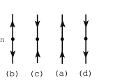
Figure 1: Vertex representation of the matrix elements of the $L$-operator.

Matrix elements of the monodromy matrix (16) are expressed then as sums over all possible configurations of arrows with different boundary conditions on a one-dimensional lattice with $M+1$ sites (see FIG. 2). Namely, operator $B(u)$ corresponds to the boundary conditions when arrows on the top and bottom of the lattice are pointing outward (configuration (B)). Operator $C(u)$ corresponds to the boundary conditions when arrows on the top and bottom of the lattice are pointing outward (configuration (C)). Operators $A(u)$ and $D(u)$ correspond to the boundary conditions when arrows on the top and bottom of the lattice are pointing up and down respectively (configurations (A) and (D)):

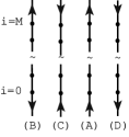
Figure 2: Matrix elements of the monodromy matrix $T(u)$.

For example an operator $B(u)$ on the lattice of three sites $(M=2)$ is: $B(u)=\phi_{0}^{\dagger}u^{-2}+\phi_{0}^{\dagger}\phi_{1}\phi_{2}^{\dagger}+u^{2}\phi_{2}^{\dagger}+\phi_{1}^{\dagger},$ and may be represented in a form (see FIG. 3).

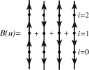
Figure 3: Vertex representation of the operator $B(u)$.

IV Scalar products and plane partitions

Recall that a partition $\lambda=(\lambda_{1},\lambda_{2},...,\lambda_{N})$ is a non-increasing sequence of non-negative integers $\lambda_{1}\geq\lambda_{2}\geq...\geq\lambda_{N}$ called the parts of $\lambda$. The sum of the parts of $\lambda$ is denoted by $|\lambda|$.

A plane partition is an array $\pi_{ij}$ of non-negative integers that are non-increasing as functions of both $i$ and $j$ $(i,j=1,2,...).$ The integers $\pi_{ij}$ are called the parts of the plane partition, and $|\pi|=\sum\pi_{ij}$ is its volume. The plane partitions are often interpreted as stacks of cubes (three-dimensional Young diagrams). The height of a stack with coordinates $ij$ is $\pi_{ij}.$ If we have $i\leq r,j\leq s$ and $\pi_{ij}\leq t$ for all cubes of the plane partition, it is said that the plane partition is contained in a box with side lengths $r,s,t.$ The symmetric plane partition is the plane partition for which $\pi_{ij}=\pi_{ji}$. In (FIG. 4) the diagram corresponding to the boxed plane partition $4\times 4\times 5$

$$\pi=\left(\begin{array}[]{cccc}5&3&3&2\\ 5&2&1&1\\ 4&1&1&0\\ 3&1&1&0\end{array}\right)$$ (31)

is represented.

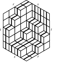
Figure 4: A plane partition with a gradient lines.

A plane partition in a $r\times s\times t$ box is equivalent to a lozenge tiling of an $(r,s,t)$-semiregular hexagon. The term lozenge refers to a unit rhombi with angles of $\frac{\pi}{3}$ and $\frac{2\pi}{3}.$

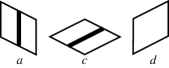
Figure 5: Three types of lozenges.

To each plane partition we can put into correspondence a $q-$weight $q^{|\pi|}$. Notice that these $q$ are not in any way related to the $q$-deformation parameter of Section II. The sum of $q-$weights of all plane partitions contained in a box $r\times s\times t$ is known as $q-$enumeration of plane partitions or the partition function of Young diagrams

$$Z_{q}(r,s,t)=\sum_{p.p}q^{|\pi|}=\prod_{i=1}^{r}\prod_{j=1}^{s}\prod_{k=1}^{t}\frac{1-q^{i+j+k-1}}{1-q^{i+j+k-2}}=\prod_{j=1}^{r}\prod_{k=1}^{s}\frac{1-q^{t+j+k-1}}{1-q^{k+j-1}}.$$ (32)

This formula is MacMahon generation function for the boxed plane partitions bres , macd . In the $q\rightarrow 1$ limit this formula gives the number of the plane partitions containing in a box $r\times s\times t$.

Let us consider the scalar product of the state vectors (29) and (30):

$$S(N,M|\{v\},\{u\})=\langle 0|\prod_{j=1}^{N}C(v_{j})\prod_{j=1}^{N}B(u_{j})|0\rangle,$$ (33)

where $\{u\}$ and $\{v\}$ are the sets of independent parameters. We shall show that after the parametrization

$$u_{j}=q^{\frac{(j-1)}{2}},\,\,v_{j}=q^{-\frac{j}{2}},\,$$ (34)

the scalar product (33) is the generating function (32) of the plane partitions containing in a box $N\times N\times M$:

$$q^{\frac{N^{2}M}{2}}\langle 0|\prod_{j=-1}^{-N}C(q^{\frac{j}{2}})\prod_{j=1}^{N}B(q^{\frac{j-1}{2}})|0\rangle=Z_{q}(N,N,M).$$ (35)

To make a connection of the scalar product (33) with the problem of enumeration of boxed plane partitions we shall use a graphic representation of its elements introduced in the previous Section. Consider a two-dimensional square lattice with $2N\times(M+1)$ sites. First $N$ vertical rows of the lattice are associated with the operators $C(v_{j})$ and the last $N$ vertical rows with operators $B(u_{j})$ (see FIG. 1 and FIG. 2). The horizontal rows of the lattice are associated with the local Fock spaces, $i$-th raw with the $i$-th space respectively. Each horizontal edge of a lattice is labelled then with an occupation number $n_{j}$ of a correspondent Fock vector $|n_{j}\rangle_{i}.$ The scalar product (33) is equal to the sum over all allowed configurations on a square lattice with the arrows on the first $N$ vertical rows pointing inwards, on the last $N$ ones pointing outwards; on the right and on the left boundaries all occupation numbers are zeros.

These configurations may be represented in terms of the lattice paths. The allowed configurations are then the number of possible non-crossing $N$ paths starting from the down left $N$ lattice edges $(-N;0),(-N+1;0),...,(-1;0)$ and ending at the $N$ top right ones $(1;M),(2;M),...,(N;M)$. The $m-$th path is running from $(-N+m-1;0)$ to $(m;M)$, $1\leq m\leq N$. In the vertical direction paths follow the arrows, and only one path is allowed on a vertical lattice edge but any number of paths can share the horizontal ones. The number of paths sharing a horizontal edges is equal to the corresponding occupation number of the edge. The length of the paths is $(N+M).$ One of the possible configurations is represented in (FIG. 6).

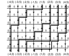
Figure 6: A typical configuration of admissible lattice paths.

The cells of the lattice under the $m-$th path may be considered as diagram of corresponding partition and may be thought of as the $m-$th column in the array $(\pi_{i,j})$. The configuration of the paths in (FIG. 6) corresponds to the plane partition in (FIG. 4) and respectively to the array (31).

On the other hand we can associate the vertical and horizontal edges carrying paths with lozenges. Lozenge ($a$) in (FIG. 5) corresponds to a vertical line of the path, while lozenge ($c$) to a horizontal one. Lattice edges without the paths correspond to a lozenge ($d$). The lozenge tiling is simply the projection of three-dimensional Young diagram with gradient lines. This establishes the mapping of the configurations generated by the scalar product (33) on the plane partitions.

Consider the scalar product (33). Due to commutation relations (23) it is a symmetric function of $N$ variables $v_{j}$ and also a symmetric function of $N$ variables $u_{j}.$ It is easy to verify that the number of operators $C(u)$ should be equal to the number of operators $B(u),$ otherwise the scalar product is equal to zero. The scalar product is evaluated by means of commutation relations (20)-(22). In the simplest case ($N=1$) the scalar product is equal to

$$S(1,M|v,u) = \langle 0|C(v)B(u)|0\rangle$$

$$= g(v,u)\left\{a(v)d(u)-a(u)d(v)\right\}$$

$$= \left\{\left(\frac{u}{v}\right)^{M+1}-\left(\frac{u}{v}\right)^{-M-1}\right\}\times\frac{1}{\frac{u}{v}-\left(\frac{u}{v}\right)^{-1}},$$

where $g(u,v)$ is the element of $R$-matrix (14) and $a(u)$ and $d(u)$ are the eigenvalues of $A(u)$ and $D(u)$ (28).

For the arbitrary $N$ one may get kbi , bik :

$$S(N,M|\{v\},\{u\}) = \langle 0|\prod_{j=1}^{N}C(v_{j})\prod_{j=1}^{N}B(u_{j})|0\rangle$$

$$= \left\{\prod_{j>k}\left(\frac{v_{k}}{v_{j}}-\frac{v_{j}}{v_{k}}\right)^{-1}\prod_{l>m}\left(\frac{u_{l}}{u_{m}}-\frac{u_{m}}{u_{l}}\right)^{-1}\right\}\det H,$$ (36)

where the matrix elements of $N\times N$ matrix $H$ are equal to

$$H_{jk}=\left\{\left(\frac{u_{k}}{v_{j}}\right)^{M+N}-\left(\frac{u_{k}}{v_{j}}\right)^{-M-N}\right\}\times\frac{1}{\frac{u_{k}}{v_{j}}-\left(\frac{u_{k}}{v_{j}}\right)^{-1}}.$$ (37)

The parametrization (34) transforms the scalar product into

$$S(N,M|\{q\})=(-1)^{\frac{N(N-1)}{2}}\left\{\prod_{j>k}\left(q^{\frac{j-k}{2}}-q^{-\frac{j-k}{2}}\right)^{-2}\right\}\det{\cal H},$$ (38)

where

$${\cal H}_{jk}=\frac{s^{\frac{k+j-1}{2}}-s^{-\frac{k+j-1}{2}}}{q^{\frac{k+j-1}{2}}-q^{-\frac{k+j-1}{2}}},$$ (39)

with $s=q^{M+N}.$ The determinant of the matrix ${\cal H}$ was considered in kup in connection with the alternating sign matrices enumeration problem and is equal to

$$\det{\cal H}=(-1)^{\frac{N(N-1)}{2}}\left\{\prod_{j>k}\left(q^{\frac{j-k}{2}}-q^{-\frac{j-k}{2}}\right)^{2}\right\}\prod_{1\leq j,k\leq N}\frac{s^{\frac{1}{2}}q^{\frac{j-k}{2}}-s^{-\frac{1}{2}}q^{-\frac{j-k}{2}}}{q^{\frac{k+j-1}{2}}-q^{-\frac{k+j-1}{2}}}.$$ (40)

Therefore,

$$S(N,M|\{q\}) = q^{-\frac{N^{2}M}{2}}\prod_{1\leq j,k\leq N}\frac{1-q^{N+M+j-k}}{1-q^{k+j-1}}$$

$$= q^{-\frac{N^{2}M}{2}}\prod_{1\leq j,k\leq N}\frac{1-q^{M-1+j+k}}{1-q^{k+j-1}}.$$ (41)

Finally, we have obtained the equality (35) for the scalar product:

$$\langle 0|C(q^{-\frac{N}{2}})...C(q^{-1})C(q^{-\frac{1}{2}})B(1)B(q^{\frac{1}{2}})...B(q^{\frac{N-1}{2}})|0\rangle=q^{-\frac{N^{2}M}{2}}Z_{q}(N,N,M).$$ (42)

V Coordinate form of state vectors and Schur functions

Using the explicit form of the operators $B(\lambda)$ we may rewrite the $N-$particle state vector (29) in the ”coordinate” form

$$|\Psi_{N}(u_{1},u_{2},...,u_{N})\rangle=\prod_{k=1}^{N}B(u_{k})|0\rangle=\sum_{{0\leq n_{0},n_{1},...,n_{M}\leq N\atop n_{0}+n_{1}+...+n_{M}=N}}f_{\{n\}}(u_{1},u_{2},...,u_{N})\prod_{j=0}^{M}|n_{j}\rangle_{j},$$ (43)

with the function $f$ equal to

$$f_{\{n\}}(u_{1},u_{2},...,u_{N})=f_{(n_{j_{1}},n_{j_{2},}...,n_{j_{M}})}(u_{1},u_{2},...,u_{N})=\sum_{{\cal B}}u_{1}^{t_{1}^{d}-t_{1}^{a}}u_{2}^{t_{2}^{d}-t_{2}^{a}}\cdot...\cdot u_{N}^{t_{N}^{d}-t_{N}^{a}}.$$ (44)

Here the sum is taken over all admissible $N$ paths with $n_{j_{1}}$ paths starting from $(1;j_{1})$, $n_{j_{2}}$ from $(1;j_{2})$, and $n_{j_{M}}$ from $(1;j_{M})$ respectively, $j_{1}>j_{2}>...>j_{M};n_{j_{1}}+...+n_{j_{M}}=N,\,n_{j_{k}}\neq 0$. The power $t_{k}^{d}$ is equal to the number of the $d(u)$ vertices in the $k-$th vertical line of the grid, while $t_{k}^{a}$ is equal to the number of $a(u)$ vertices respectively.

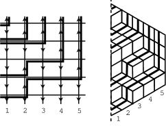
Figure 7: Lattice paths representation of a particular term of the 5-particle state vector, and a correspondent part of a plane partition.

The following representation is valid

$$f_{\{n\}}(u_{1},u_{2},...,u_{N})=\left(u_{1}u_{2}\cdot...\cdot u_{N}\right)^{-M}S_{\{\lambda\}}(u_{1}^{2},u_{2}^{2},...,u_{N}^{2}),$$ (45)

where $S_{\{\lambda\}}(u_{1},u_{2},...,u_{N})$ is the Schur function

$$S_{(\lambda_{1},...,\lambda_{N})}(u_{1},u_{2},...,u_{N})=\frac{\det\left(u_{j}^{N-i+\lambda_{i}}\right)}{\prod_{1\leq i<j\leq N}(u_{i}-u_{j})},$$ (46)

and there is one to one correspondence between the occupation number configuration $\{n\}$ and partitions $\{\lambda\}$:

$$\{n\} = (n_{j_{1}},n_{j_{2},}...,n_{j_{M}})\Longleftrightarrow\{\lambda\}=(\lambda_{1},...,\lambda_{N})$$ (47)

$$\lambda_{k} = j_{1};\,\,\,1\leq k\leq n_{j_{1}}$$

$$\lambda_{k} = j_{2};\,\,\,n_{j_{1}}+1\leq k\leq n_{j_{2}}+n_{j_{1}}$$

$$\ \ \ \ \ \ \ ...$$

$$\lambda_{k} = j_{N};\,\,\,n_{j_{1}}+...+n_{j_{M-1}}+1\leq k\leq n_{j_{1}}+...+n_{j_{M}}=N.$$

The state conjugated to (43) is

$$\langle\Psi_{N}(u_{1},u_{2},...,u_{N})|=\langle 0|\prod_{k=1}^{N}C(u_{k})=\sum_{{0\leq n_{0},n_{1},...,n_{M}\leq N\atop n_{0}+n_{1}+...+n_{M}=N}}f_{\{n\}}(u_{1}^{-1},u_{2}^{-2},...,u_{N}^{-2})\prod_{j=0}^{M}\langle n_{j}|_{j},$$ (48)

with

$$f_{\{n\}}(u_{1}^{-1},u_{2}^{-2},...,u_{N}^{-2})=\sum_{{\cal C}}u_{1}^{t_{1}^{d}-t_{1}^{a}}u_{2}^{t_{2}^{d}-t_{2}^{a}}\cdot...\cdot u_{N}^{t_{N}^{d}-t_{N}^{a}},$$ (49)

where the sum is taken over all admissible $N$ paths with $n_{j_{1}}$ paths ending at $(-1;j_{1})$, $n_{j_{2}}$ ending at $(-1;j_{2})$, and $n_{j_{M}}$ ending at $(1;j_{M})$ respectively, $j_{1}>j_{2}>...>j_{M};n_{j_{1}}+...+n_{j_{M}}=N,\,n_{j_{k}}\neq 0$.

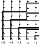
Figure 8: Lattice paths representation of a particular term of the conjugated state vector.

Due to the orthogonality of the Fock states (17) the scalar product is equal to

$$S(N,M|\{v\},\{u\})=\langle\Psi_{N}(v_{1},v_{2},...,v_{N})|\Psi_{N}(u_{1},u_{2},...,u_{N})\rangle$$

$$=\sum_{{0\leq n_{0},n_{1},...,n_{M}\leq N\atop n_{0}+n_{1}+...+n_{M}=N}}f_{\{n\}}(v_{1}^{-1},v_{2}^{-1},...,v_{N}^{-1})f_{\{n\}}(u_{1},u_{2},...,u_{N})$$

$$=\sum_{{0\leq n_{0},n_{1},...,n_{M}\leq N\atop n_{0}+n_{1}+...+n_{M}=N}}\sum_{{\cal C}}v_{1}^{t_{1}^{d}-t_{1}^{a}}v_{2}^{t_{2}^{d}-t_{2}^{a}}\cdot...\cdot v_{N}^{t_{N}^{d}-t_{N}^{a}}\sum_{{\cal B}}u_{1}^{t_{1}^{d}-t_{1}^{a}}u_{2}^{t_{2}^{d}-t_{2}^{a}}\cdot...\cdot u_{N}^{t_{N}^{d}-t_{N}^{a}}.$$ (50)

Taking into account the representation (45) we can express the scalar product in terms of Schur functions

$$S(N,M|\{v\},\{u\})=\left(\prod_{j=1}^{N}\frac{v_{j}^{M}}{u_{j}^{M}}\right)\sum_{\lambda\subseteq\{M^{N}\}}S_{\{\lambda\}}(u_{1}^{2},u_{2}^{2},...,u_{N}^{2})S_{\{\lambda\}}(v_{1}^{-2},v_{2}^{-2},...,v_{N}^{-2}),$$ (51)

where the sum is over all partitions, $\lambda$ , into at most $N$ parts each of which is less than or equal to $M$. Comparing this formula with (36) we obtain the following determinantal expression

$$\ \ \sum_{\lambda\subseteq\{M^{N}\}}S_{\{\lambda\}}(x_{1}^{2},x_{2}^{2},...,x_{N}^{2})S_{\{\lambda\}}(y_{1}^{2},y_{2}^{2},...,y_{N}^{2})$$ (52)

$$= \left(\prod_{j=1}^{N}x_{j}^{M}y_{j}^{M}\right)\left\{\prod_{j>k}\frac{y_{j}y_{k}}{y_{j}^{2}-y_{k}^{2}}\prod_{l>m}\frac{x_{l}x_{m}}{x_{l}^{2}-x_{m}^{2}}\right\}\det H,$$

where the matrix $H$ is (37)

$$H_{jk}=\left\{\left(x_{k}y_{j}\right)^{M+N}-\left(x_{k}y_{j}\right)^{-M-N}\right\}\times\frac{1}{x_{k}y_{j}-\left(x_{k}y_{j}\right)^{-1}}.$$

The volume $|\pi|$ of the plane partition $\pi$ in a box $(N\times N\times M)$ may be expressed as

$$2|\pi|=N^{2}M+\sum_{k=-1}^{-N}k\left(l_{k}^{d}-l_{k}^{a}\right)+\sum_{j=1}^{N}(j-1)\left(l_{j}^{d}-l_{j}^{a}\right),$$ (53)

where the first sum in this equality is over the columns going along the ”$s$” side of hexagon while the second one is over the columns along the ”$r$” side respectively, and $l_{j}^{a,d}$ is the number of lozenge of type $a,d$ (see FIG. 5) in the $j$-th column of the hexagon. It may be checked that $l_{j}^{d}-l_{j}^{a}=t_{j}^{d}-t_{j}^{a}$. The substitution of the parametrization (34) into the equation (50) gives for the scalar product

$$S(N,M|\{q\}) = \langle\Psi_{N}(q^{-\frac{1}{2}},q^{-1},...,q^{-\frac{N}{2}})|\Psi_{N}(1,q,...,q^{\frac{N-1}{2}})\rangle$$

$$= q^{-\frac{N^{2}M}{2}}\sum_{p.p}q^{|\pi|}.$$

Together with (41) this equation provides us with the proof of MacMahons enumeration formula for the boxed plane partitions within the frames of Quantum Inverse Method.

From the equation (51) we obtain the equality kratt :

$$\sum_{\lambda\subseteq\{M^{N}\}}S_{\{\lambda\}}(1,q,...,q^{N-1})S_{\{\lambda\}}(q,q^{2},...,q^{N})=\sum_{p.p}q^{|\pi|}.$$

The parts $\lambda_{k}$ of the partition $\lambda$ (47) may be considered as the coordinates of the particles (the coordinate $\lambda_{k}$ corresponds to the $k$-th particle). The state of the system is spanned by the orthonormal basis $|\lambda\rangle=|\lambda_{1},\lambda_{2},...,\lambda_{m}\rangle:\,\,\langle\mu|\lambda\rangle=\delta_{\{\mu\},\{\lambda\}}$. The $N$-particle state vector (43) is given then by the equation

$$|\Psi_{N}(u_{1},u_{2},...,u_{N})\rangle=\left(u_{1}u_{2}\cdot...\cdot u_{N}\right)^{-M}\sum_{\lambda\subseteq\{M^{N}\}}S_{\{\lambda\}}(u_{1}^{2},u_{2}^{2},...,u_{N}^{2})|\lambda\rangle,$$ (54)

and respectively

$$\prod_{j=1}^{N}\tilde{B}(u_{j})|0\rangle=\sum_{\lambda\subseteq\{M^{N}\}}S_{\{\lambda\}}(u_{1}^{2},u_{2}^{2},...,u_{N}^{2})|\lambda\rangle,$$ (55)

where the sum in both formulas is taken over all partitions, $\lambda$ , into at most $N$ parts each of which is less than or equal to $M$. By the construction operators $\tilde{B}(u)\equiv u^{-M}B(u)$, and $\tilde{C}(u)\equiv u^{M}C(u)$ possess the following properties

$$\tilde{B}(1)|\lambda\rangle=\sum_{\mu\supset\lambda}|\mu\rangle,\,\,\,\,\langle\lambda|\tilde{C}(1)=\sum_{\mu\supset\lambda}\langle\mu|,$$ (56)

and

$$\prod_{j=1}^{N}\tilde{B}(u_{j})|\lambda\rangle = \sum_{\mu\supset\lambda}S_{\{\mu/\lambda\}}(u_{1}^{2},u_{2}^{2},...,u_{N}^{2})|\mu\rangle,$$ (57)

$$\langle\lambda|\prod_{j=1}^{N}\tilde{C}(u_{j}) = \sum_{\mu\supset\lambda}S_{\{\mu/\lambda\}}(u_{1}^{-2},u_{2}^{-2},...,u_{N}^{-2})\langle\mu|,$$

where $S_{\{\mu/\lambda\}}(x_{1},x_{2},...,x_{N})$ is a skew Schur function indexed by a pair of partitions $\mu$ and $\lambda$ such that $\lambda\subset\mu$ macd . From this point of view operators $\tilde{B}(u)$ and $\tilde{C}(u)$ may be considered as the transition operators between the diagonals of a plane partitions.

VI Correlation functions

Let us calculate the generating function of the plain partitions contained in a box $N\times N\times M$ provided that the height $\pi_{1N}$ of the stack of the cubes is fixed and equal to $m$.

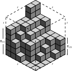
Figure 9: A Young diagram with fixed heights $\pi$ of the stack of cubes.

To find this function we have to consider a scalar product on a lattice under the condition that the $N$-th lattice path enters the $N$-th vertical line of the grid at the $m$-th row:

$$P_{1N}(m|\{v\},\{u\})=\langle 0|\prod_{j=1}^{N}C(v_{j})\prod_{j=1}^{N-1}B(u_{j})\phi_{m}^{\dagger}|0\rangle.$$ (58)

To calculate this scalar product we may use the following decomposition of the operators $B(u)$ and $C(u)$:

$$B(u)|0\rangle = u^{-M}\sum_{j=0}^{M}\phi_{j}^{\dagger}u^{2j}|0\rangle,$$ (59)

$$\langle 0|C(u) = u^{M}\langle 0|\sum_{j=0}^{M}\phi_{j}u^{-2j}.$$ (60)

The substitution of decomposition (59) into the scalar product (33) gives

$$S(N,M|\{v\},\{u\})=\sum_{m=0}^{M}(u_{N})^{-M+2m}P_{1N}(m|\{v\},\{u\}).$$ (61)

The determinant of the matrix $H$ in (36) may be developed by the last column. The comparison of the obtained decomposition with (61) leads to the equality

$$\frac{P_{1N}(m|\{v\},\{u\})}{S(N,M|\{v\},\{u\})}=\frac{(-1)^{N-1}}{(u_{N})^{N-1}}\left\{\prod_{t<N}\frac{(u_{N})^{2}-(u_{t})^{2}}{(u_{t})^{2}}\right\}\frac{\det Q}{\det H}.$$ (62)

The entries of $N\times N$ matrix $Q$ are given by

$$Q_{jN}=(v_{j})^{M+N-1-2m},\,\,\,\ Q_{jk}=H_{jk},\,\,k\neq N,$$ (63)

where $H_{jk}$ are the matrix elements (37). After the parametrization (34) we find that the probability of the height $\pi_{1N}$ to be equal to $m$ is

$$\langle m\rangle_{1N} = \frac{P_{1N}(m|\{q\})}{S(N,M|\{q\})}$$ (64)

$$= q^{-\frac{(N-1)^{2}}{2}}\left\{\prod_{t<N}\left(1-q^{N-t-2}\right)\right\}\frac{\det{\cal Q}}{\det{\cal H}},$$

where

$${\cal Q}_{jN}=q^{-\frac{j(M+N-1-2m)}{2}},\,\,\,\,{\cal Q}_{jk}={\cal H}_{jk},\,\,k\neq N,$$ (65)

and ${\cal H}_{jk}$ are the matrix elements (39). It is evident that this expectation value is the same for the height $\pi_{N1}$ in the opposite corner of the diagram.

The correlation function of the heights of the columns $\pi_{1N},\pi_{N1}$ at the opposite sides of the Young diagram (see FIG. 9) may be obtained from the following scalar product

$$P_{N1;1N}(n;m|\{v\},\{u\})=\langle 0|\phi_{n}\prod_{j=1}^{N-1}C(v_{j})\prod_{j=1}^{N-1}B(u_{j})\phi_{m}^{\dagger}|0\rangle.$$ (66)

The scalar products (61) and (66) may be expressed in terms of the skew Schur functions (57) as well.

The other function of interest is the projection of the Bethe wave function $\prod_{j=1}^{N}B(u_{j})|0\rangle$ on the ”steady state” vector:

$$|P\rangle=\sum_{{0\leq n_{0},n_{1},...,n_{M}\leq N\atop n_{0}+n_{1}+...+n_{M}=N}}\prod_{j=0}^{M}|n_{j}\rangle_{j}.$$ (67)

From the representation (43) and relation (45) we obtain the equality

$$\langle P|\prod_{j=1}^{N}B(u_{j})|0\rangle=\left(u_{1}u_{2}\cdot...\cdot u_{N}\right)^{-M}\sum_{\lambda\subseteq\{M^{N}\}}S_{\{\lambda\}}(u_{1}^{2},u_{2}^{2},...,u_{N}^{2}),$$ (68)

where the sum is over all partitions, $\lambda$ , into at most $N$ parts each of which is less than or equal to $M$. It is known that bres

$$\sum_{\lambda\subseteq\{M^{N}\}}S_{\{\lambda\}}(x_{1},x_{2},...,x_{N}) = \frac{\det\left(x_{i}^{j-1}-x_{i}^{M+2N-j}\right)}{\det\left(x_{i}^{j-1}-x_{i}^{2N-j}\right)}$$

$$= \prod_{i=1}^{N}\frac{1}{1-x_{i}}\prod_{1\leq i<j\leq N}\frac{1}{1-x_{i}x_{j}},$$

and we obtain for the projection (68)

$$\langle P|\prod_{j=1}^{N}B(u_{j})|0\rangle=\prod_{i=1}^{N}\frac{1}{1-u_{i}^{2}}\prod_{1\leq i<j\leq N}\frac{1}{1-u_{i}^{2}u_{j}^{2}}.$$ (70)

By the construction the considered correlation function is the generating function of the symmetric plane partitions, the plane partitions satisfying the condition $\pi_{ij}=\pi_{ji}$. From (44) and the relation $t_{k}^{d}-t_{k}^{a}=l_{k}^{d}-l_{k}^{a}$ it follows that

$$\langle P|\prod_{j=1}^{N}B(u_{j})|0\rangle=\sum_{{\cal B}}u_{1}^{l_{1}^{d}-l_{1}^{a}}u_{2}^{l_{2}^{d}-l_{2}^{a}}\cdot...\cdot u_{N}^{l_{N}^{d}-l_{N}^{a}}.$$

The volume of the symmetric plane partitions may be expressed as

$$2|\pi|_{sym}=N^{2}M+\sum_{j=1}^{N}(2j-1)\left(l_{j}^{d}-l_{j}^{a}\right),$$ (71)

where the sum is over the columns going along the ”$r$” side of the hexagon. Then

$$\langle P|\prod_{j=1}^{N}B(q^{\frac{2j-1}{2}})|0\rangle=q^{-\frac{N^{2}M}{2}}\sum_{sym}q^{|\pi|},$$

and we obtain the well known result for the generating function of the symmetric plane partitions

$$\sum_{\lambda\subseteq\{M^{N}\}}S_{\{\lambda\}}(q,q^{3},...,q^{2N-1})=\sum_{sym}q^{|\pi|}.$$

Till now we have considered plane partitions in a box with $r=s$. To study the general case when $r\neq s$ we have to consider the following scalar products

$$S^{A}(N,L,M|\{v\},\{u\},\{u^{A}\}) = \langle 0|\prod_{j=1}^{N}C(v_{j})\prod_{j=1}^{L}A(u_{j}^{A})\prod_{j=1}^{N}B(u_{j})|0\rangle,$$ (72)

$$S^{D}(N,L,M|\{v\},\{u\},\{u^{D}\}) = \langle 0|\prod_{j=1}^{N}C(v_{j})\prod_{j=1}^{L}D(u_{j}^{D})\prod_{j=1}^{N}B(u_{j})|0\rangle.$$ (73)

Following the mapping introduced in this Section it may be shown that these averages are the generating functions of plane partitions in a box $r\times s\times t$ with $r=N,s=N+L,t=M$ for (72), and $r=N+L,s=N,t=M$ for (73).

VII Boxed plane partitions and Toda lattice

The $N\times N$ matrix ${\cal H}$ (39) is a Hänkel matrix with the matrix elements

$${\cal H}_{jk}=h(q^{j+k-1}),$$ (74)

where

$$h(q)=\frac{q^{\frac{M+N}{2}}-q^{-\frac{M+N}{2}}}{q^{\frac{1}{2}}-q^{-\frac{1}{2}}}.$$ (75)

By the successive subtraction of columns the determinant of this matrix may be brought into the form

$$\det{\cal H} = \det h,$$ (76)

$$h_{jk} = D_{q}^{j+k-2}h(q),$$

and $D_{q}$ is the $q$-difference operator:

$$D_{q}f(z)=f(qz)-f(z).$$ (77)

Following the standard procedure ick , ikk it may be shown that the function $\tau(N,M;q)\equiv\det{\cal H}$ satisfies the equation

$$D_{q}^{2}\ln\tau(N,M;q)=\frac{\tau(N+1,M;q)\tau(N-1,M;q)}{\tau^{2}(N,M;q)},$$ (78)

which, after the substitution

$$\rho(N;q)=\ln\frac{\tau(N+1,M;q)}{\tau(N,M;q)}$$

becomes the $q$-difference Toda equation:

$$D_{q}^{2}\rho(N;q)=e^{\rho(N+1;q)-\rho(N;q)}-e^{\rho(N;q)-\rho(N-1;q)}.$$ (79)

The role of time plays the deformation parameter $q$.

VIII Acknowledgments

I would like to thank N.Yu. Reshetikhin, A.M. Vershik, and A.G. Pronko for valuable discussions. This work was partially supported by CRDF grant RUM1-2622-ST-04 and RFBR project 04-01-00825.

References

(1) G.E. Andrews, The theory of partitions
(Cambridge University Press, Cambridge, 1998).
(2) A. Vershik, talk at the 1997 conference on Formal Power Series and
Algebraic Combinatorics, Vienna.
(3) A. Vershik and S. Kerov, Asymptotics of the Plancherel measure of the
symmetric group and the limit form of Young tableaux, Soviet
Math. Dokl. 18, 527 (1977).
(4) H. Cohn, M. Larsen, and J. Propp, The shape of a typical boxed plane partition,
New York J. of Math. 4, 137 (1998).
(5) H. Cohn, R. Kenyon, and J. Propp, A variational principle for
domino tilings, J. Amer. Math. Soc. 14, 297 (2001).
(6) A. Okounkov and N. Reshetikhin, Correlation function
of Schur process with application to local geometry of a random
3-dimensional Young diagram, J. American Math. Soc. 16, 58
(2003).
(7) P.L. Ferrari and H. Spohn, Step functions for a
faceted crystal, J. Stat. Phys. 113, 1 (2003).
(8) R. Rajesh and D. Dhar, An exactly solvable
anisotropic directed percolation model in three dimensions, Phys.
Rev. Lett. 81, 1646 (1998).
(9) A. Okounkov, N. Reshetikhin, and C. Vafa, Quantum
Calabi-Yau and classical crystals, hep-th/0309208.
(10) L.D. Faddeev, N. Yu. Reshetikhin, L.A. Takhtajan, Quantization
of Lie groups and Lie algebras, Leningrad. Math. J. 1, 193
(1990).
(11) P.P. Kulish and E.V. Damaskinsky, On the
-oscillator and the quantum algebra , J. Phys. A:
Math. Gen. 23, L415 (1990).
(12) M. Kashivara, Crystalizing the -analogue of universal enveloping algebras,
Commun. Math. Phys. 133, 249 (1990).
(13) G. Lusztig, Introduction to quantum groups, Progr. in Math. 110,
(Birkhauser, 1993).
(15) V.E. Korepin, N.M. Bogoliubov, and A.G. Izergin, Quantum Inverse Scattering Method and Correlation Functions (Cambridge University Press, Cambridge, 1993).
(16) N.M. Bogoliubov, R.K. Bullough, and J. Timonen, Critical behavior for correlated strongly coupled boson systems in
1+1 dimensions, Phys. Rev. Lett. 25, 3933 (1994).
(17) N.M. Bogoliubov and T. Nassar, On the spectrum of the
non-Hermitian phase-difference model, Phys. Lett. A 234,
345 (1997).
(18) N.M. Bogoliubov, A.G. Izergin, and N.A. Kitanine, Correlation functions for a strongly correlated boson systems,
Nucl. Phys. B 516, 501 (1998).
(20) D.M. Bressoud, Proofs and Confirmations. The Story
of the Alternating Sign Matrix Conjecture, (Cambridge University
Press, Cambridge, 1999).
(21) I. G. Macdonald, Symmetric functions and Hall
polynomials, (Clarendon Press, 1995).
(22) G. Kuperberg, Another proof of the
alternating-sign matrix conjecture, Int. Math. Res. Not. 1996, 139 (1996).
(23) C. Krattenthaller, The major counting of
nonintersecting lattice paths and generating functions of
tableaux, Mem. Amer. Math. Soc. 115, 552 (1995).
(24) A.G. Izergin , D.A. Coker, and V.E. Korepin, Determinant formula for the six-vertex model, J. Phys. A: Math.
Gen. 25, 4315 (1992).
(25) A. G. Izergin, E. Karjalainen, and N.A. Kitanine, Integrable equations for the partition function of the six-vertex
model, J. Math. Sci. 100, 2141 (2000).