Mean-field glass transition in a model liquid

Abstract

We investigate the liquid-glass phase transition in a system of point-like particles interacting via a finite-range attractive potential in $D$-dimensional space. The phase transition is driven by an ‘entropy crisis’ where the available phase space volume collapses dramatically at the transition. We describe the general strategy underlying the first-principles replica calculation for this type of transition; its application to our model system then allows for an analytic description of the liquid-glass phase transition within a mean-field approximation, provided the parameters are chosen suitably. We find a transition exhibiting all the features associated with an ‘entropy crisis’, including the characteristic finite jump of the order parameter at the transition while the free energy and its first derivative remain continuous.

I Introduction

Notable progress in understanding fundamental aspects of structural glasses and their freezing transition has been made glass ; significant advancements originate from the dynamic formulation of the glass transition using mode coupling theory modecoupling , while the statistical mechanics approach draws extensively from the analogy between the well studied spin-glass mpv and the glassy solid K . While the spin glass is characterized by random frozen orientations of spins due to the presence of quenched disorder, the structural glass is characterized by random frozen space positions of the particles but does not rely on the presence of quenched disorder. A central idea put forward in this context is the concept of the ‘entropy crisis’ GibbsDiMarzio driving the transition into the glassy state through a collapse of the system’s phase space. Transitions of this type have shown up in various disordered systems rem ; 1rsb and in the ‘discontinuous’ spin-glasses containing no quenched disorder repl (see also Ref. glass1 for similar systems with other then spin degrees of freedom). In this paper, we apply a heuristic frameworkMP based on an ‘entropy crisis’ scenario to describe the liquid-glass transition and the low-temperature thermodynamics of the glassy state in a system of interacting particles in $D$-dimensional space.

Progress in our understanding of the liquid-glass phase transition and the physics of the low-temperature glass state is made along two avenues: i) experimental and numerical studies provide new details on specific materials and on model systems but have little impact on our general understanding of the glass phenomenon. On the other hand, ii) conceptual studies push our general understanding but unfortunately provide little predictive power when it comes to the description of realistic systems. In choosing a suitable model system, we then have to compromise between a realistic description of the glass former and one allowing us to make analytical progress, e.g., within a mean-field approach. The first model describing a liquid-glass phase transition and allowing for a mean-field type analysis was proposed by Kirkpatrick and Thirumalai KT . Formulated within a density functional theory, it provided a consistent static and dynamic description of the structural glass transition. New insights into the nature of the glass transition based on studies of coupled replicated glassy systems Monasson ; FranzParisiCardenas led to the formulation of a first principles computational scheme providing a description of the equilibrium thermodynamics of glasses MP . This scheme has been successfully applied, combining analytical and numerical techniques, to the soft-spheres model in three dimensions MP and to the Lennard-Jones binary mixture CPV . Recently, a model with point-like particles interacting via a spatially oscillating infinite-range potential has been analyzed within this framework mfg1 . Despite its unrealistic structure, this model turned out to provide a good testbed for the replica based approach: the physics of the liquid-glass phase transition revealed in this model turned out fully consistent with the heuristic ideas of the ‘entropy crisis’ scenario. In the present paper, we consider a much more realistic model of a structural glass: adopting again the scheme suggested in Ref. MP, , we study the low-density limit of a system of particles in $D$-dimensional space interacting via a finite-range attractive potential of depth $U_{0}$, confined to a shell of radius $R$ and thickness $2r_{0}$, see Fig. 1. It turns out, that an appropriate choice of the interaction parameters ($r_{0}\ll R$) allows us to adopt a mean-field approximation and proceed with an analytic calculation of the free energy and a properly defined order parameter to the very end. We then arrive at a complete analytic description of the liquid-glass phase transition occurring in this model glass former and demonstrate that it is again consistent with the ‘entropy crisis’ scenario.

Figure 1: Interaction potential between particles used in our model glass former. The attractive interaction (normalized to unity) is limited to a shell of width $2r_{0}$ at a radius $R\gg r_{0}\gg 1$, where we have set the particle radius to unity. The repulsive core prevents the collapse of the system into two clusters.

In spite of this success, we have to admit ignoring various important issues related to the structural glass transition: First, we explicitly avoid the discussion of the relevance of our equilibrium statistical mechanical approach for the apparently non-equilibrium type liquid-glass phase transition. This question is both general and deep and we are unable to present an answer at the present stage. Rather, we hope that, like in the case of spin-glasses (another example of matter residing in a non-equilibrium state), at least some of the physical phenomena and observables are well defined and make proper physical sense even when computed in terms of an equilibrium approach. Second, we also prefer not to start a lengthy (and useless) discussion of the question, what to do with the crystal state. Such a crystalline state is certainly present in our model and, since its energy is evidently lower than the typical energy of glassy configurations, it is the true ground state of the system. In fact, this is the typical situation for most models of glasses and the usual algorithm of treating the presence of the crystal state (which we also follow in this paper) is simple: it has to be ignored. On a qualitative level, the reason for such a pragmatic approach is very simple: it is well known that frozen glassy states do exist at low temperatures regardless of the presence of the crystal ground state. Moreover, in many circumstances such states turn out to be quite stable during reasonable observation times; we then can safely assume that the crystal state is located far away from the relevant glassy states in configurational space and furthermore that the crystal and glassy states are separated by large energy barriers. This is a quite standard situation in statistical mechanics: except for some rare cases admitting an exact solution, one usually studies only a limited ad hoc chosen part of the phase space depending on the object under study. In the case of the structural glass, one then expects two scenaria: either the basic assumption (that the existence of the crystal can be ignored) turns out to be reasonable and the crystal configurations never show up in the calculations. Or, this assumption is wrong and then one inevitably faces some kind of instabilities and divergences. As for the model and method considered in the present paper, the calculations demonstrate that the crystal state indeed does not interfere with the glassy configurations.

The paper is structured as follows: In section II below, we first describe the heuristic framework underlying our replica analysis along the lines discussed in Ref. MP, and introduce our specific model. Its free energy is calculated within the replica mean-field approach in section III. The results and conclusions are given in section IV: We find that the system freezes at the glass temperature $T_{c}=U_{0}/\ln(R/r_{0})$ into an amorphous solid with a number of nearest neighbors slightly larger than $D$. We determine the order parameter and its jump at $T_{c}$ and present analytical expressions for the free energy and entropy of the solid and liquid phases as well as for the configurational entropy or complexity.

II Structural glass transition

II.1 Symmetry breaking in random systems

Consider a system of $N$ particles in $D$-dimensional space described by the Hamiltonian

$$H[{\bf x}_{i}]=\frac{1}{2}\sum_{i,j=1}^{N}U(|{\bf x}_{i}-{\bf x}_{j}|),$$ (1)

where ${\bf x}_{i}$ denotes the position of the $i$-th particle and $U(|{\bf x}|)$ is the interparticle potential. We assume that at low temperatures the system is frozen in a disordered (glassy) state which is characterised by random spatial positions of the particles; this can be achieved through a rapid quench avoiding the crystallization by entropic reasons. The glass state is characterized by broken translational and rotational symmetries, but unlike the ordered crystal configurations (characterized by their specific spatial and rotational symmetries), it is impossible to identify the residual symmetries left in the glassy state. This naturally resembles the spin-glass problem, where the spins are frozen in a random state which cannot be characterized by any apparent global symmetry breaking. However, unlike spin-glasses, here we do not have quenched disorder installed in the initial Hamiltonian. Nevertheless, the ideas borrowed from the spin-glass theory and in particular the use of the replica technique turn out to be quite fruitful also for the description of structural glasses MP .

In order to demonstrate the effect of spontaneous symmetry breaking, e.g., in ordered magnetic systems, one introduces a conjugate field coupled to the order parameter which is set to zero at the end (after taking the thermodynamic limit). In spin-glasses, the same strategy can be applied by introducing several weakly coupled copies (replicas) of the original system. Similarly, in order to demonstrate the freezing of a system of interacting particles (described by (1)) into a random glass state, we introduce two identical copies (with particles at positions ${\bf x}_{i}$ and ${\bf y}_{i}$, respectively) of the same system described the Hamiltonian

$$H_{2} = \frac{1}{2}\sum_{i,j}^{N}U(|{\bf x}_{i}-{\bf x}_{j}|)+\frac{1}{2}\sum_{i,j}^{N}U(|{\bf y}_{i}-{\bf y}_{j}|)$$ (2)

$$\qquad\qquad\qquad+\epsilon\sum_{i}^{N}W({\bf x}_{i}-{\bf y}_{i}).$$

The last term in (2) describes a weak attractive potential $W$ between the particles at ${\bf x}_{i}$ and ${\bf y}_{i}$ of the two systems and plays the role of the symmetry breaking conjugate field in the ordered system. As usual, the control parameter $\epsilon$ is set to zero after taking the thermodynamic limit and the system can end up in one of two phases: i) the particles of the two systems are independent (uncorrelated), indicating that they do not memorize their spatial positions and hence the original system is in the high-temperature liquid phase, or ii) the positions of the particles remain correlated, indicating that they are localized in space and we conclude that the original system is in the low-temperature solid state. As in spin glasses, in order to obtain more detailed information about the phase transition, it is convenient to introduce $m$ replicas of the original system. Also, in the actual calculation there is no need to introduce a supplementary attractive potential between the replicas: following standard practice, it is sufficient to allow for the possibility of symmetry breaking in order to prove its existence afterwards.

II.2 Entropy crisis scenario

The entropy crisis scenario GibbsDiMarzio for the glass transition builds on the idea of a phase space collapse upon entering the frozen phase; in its pure form it shows up in the random energy model of spin glasses which has been solved exactly rem . We first briefly summarize the main features of this heuristic framework as applied to the problem of structural glasses, following the original work of Mézard and Parisi MP .

We assume that the partition function $Z$ can be represented in the form

$$Z=\sum_{\alpha}\exp\left(-Nf_{\alpha}/T\right),$$ (3)

where $Nf_{\alpha}$ denote the energies of the thermodynamically relevant local mimima in configurational space. The number $\Omega(f)$ of local minima with energy $f$ is assumed to be exponentially large, $\Omega(f)=\exp[NS(f,T)]$, where $S(f,T)$ denotes the configurational entropy density or complexity. Finally, the function $S(f,T)$ at fixed $T$ shall have the qualitative shape shown in Fig. 2, with $S(f,T)=0$ at $f\leq f_{\mathrm{min}}(T)$, and a concave increase for $f>f_{\mathrm{min}}(T)$.

Figure 2: Qualitative shape of the configurational entropy density assumed in the phenomenological description of a glass transition driven by an entropy crisis. The slope $\beta$ corresponds to the inverse temperature and assumes its maximal value $\beta_{c}=1/T_{c}$ at the glass transition temperature $T_{c}$.

The partition function is written in the form

$$Z\approx\int_{f>f_{\mathrm{min}}}df\exp\bigl{\{}-N[f-TS(f,T)]/T\bigr{\}}$$ (4)

which can be evaluated within a saddle-point approximation in the thermodynamic limit ($N\to\infty$). The free energy density $F(T)=-T({\rm ln}Z)/N$ is given by

$$F(T)=f_{*}(T)-TS[f_{*}(T),T],\qquad T>T_{c},$$ (5)

with $f_{*}(T)$ defined via $\partial_{f}S|_{f_{*}(T)}=1/T<\beta_{c}$ and $\beta_{c}$ the maximal slope of the function $S(f)$, cf. Fig. 2. At low temperatures $T<T_{c}$ the integral is determined by the lowest energy state alone, $F(T)=f_{\mathrm{min}}(T)$.

A microscopic formalism capturing the above phenomenology can be set up with the help of replicas MP : Consider $m$ identical (non-coupled) replicas of the same system where the particle positions remain correlated among the different replicas; this Ansatz describes a molecular liquid where each molecule consists of $m$ particles originating from different replicas. The partition function of the replicated system takes the form

$$Z_{m}\approx\int_{f>f_{\mathrm{min}}}df\exp\bigl{\{}-Nm[f-(T/m)S(f,T)]/T\bigr{\}}.$$ (6)

Note that the phase space volume $\Omega(f)$ remains that of the non-replicated liquid since the molecular structure essentially preserves the configurational degrees of freedom, hence the ‘entropic temperature’ is reduced by a factor $m$. The free energy density $F(m,T)=-(T/mN)\,{\rm ln}Z_{m}$ of the molecular liquid reads

$$F(m,T)\!=\!\left\{\begin{array}[]{ll}\displaystyle{\!\!f_{*}(m,T)-\frac{T}{m}S[f_{*}(m,T),T]},&\!T>mT_{c},\\ \vskip 5.0pt\cr\!f_{\mathrm{min}}(T),&\!T<mT_{c},\end{array}\right.$$ (7)

where $f_{*}(m,T)$ is defined via the saddle-point equation

$$\partial_{f}S(f,T)\big{|}_{f_{*}(m,T)}=m/T<\beta_{c}.$$ (8)

In order to study the thermodynamic properties of our original system (with $m=1$) in the low temperature glassy phase at $T<T_{c}$, we continue analytically the expression for the free energy density $F(m,T)$ from integer values $m$ to arbitrary continuous values and analyze its behavior for $m<1$. Starting from small $m$ with $0<m<T/T_{c}\equiv m_{*}(T)$, the $m$-replica system resides in the molecular liquid phase with a free energy density given by (7). As $m$ approaches $m_{*}(T)$ from below, the free energy density becomes pinned to the lowest value $f_{\mathrm{min}}(T)$ and the system freezes into the glassy phase. A further increase of $m$ beyond $m_{*}(T)$ results in a constant free energy density $f_{\mathrm{min}}(T)$ and this remains to be the case as $m\to 1$. As a result, the free energy density (and hence the entire thermodynamics) of the original glass phase can be computed from the $m$-fold replicated system residing in the molecular liquid phase and taking the limit $F_{m=1}(T)\equiv F[m_{*}(T),T]$. The critical temperature $T_{c}$ is reached when $m_{*}(T_{c})=1$. At temperatures above $T_{c}$ the system resides in a liquid phase: replicas are independent, hence $m=1$, and the free energy is given by $F_{m=1}(T)=F[1,T]$.

The crucial step then is the determination of $m_{*}(T)$. Assume we have managed to compute the free energy density $F(m,T)$ of the $m$-replica system for the molecular liquid phase (note the crucial role of ergodicity in the liquid allowing for an unrestricted averaging over phase space; we cannot hope to do such a calculation for the amorphous solid with its restricted phase space). Provided our system indeed follows the heuristics of an entropy crisis, we can cast this free energy density into the form (7) with $f_{*}(m,T)$ the solution of the saddle-point equation (8). The critical replica parameter $m_{*}(T)$ then is determined by the condition $f_{*}(m_{*}(T),T)=f_{\mathrm{min}}(T)$ or, equivalently, $S[f_{*}(m_{*}(T)),T]=0$. Fortunately, we do not need to know a priori the form of the configurational entropy density $S(f,T)$: calculating the derivatives of the free energy density $F(m,T)$ with respect to $m$ at $m=m_{*}(T)$, we easily find that

$$\partial_{m}F(m,T)\big{|}_{m=m_{*}}\!=\big{\{}(T/m^{2})S[f_{*}(m,T),T]$$

$$\qquad\quad+\,(\partial_{m}f_{*})\,\partial_{f_{*}}\big{[}f_{*}-TS(f_{*},T)/m\big{]}\big{\}}_{m=m_{*}}\!\!\!=0$$

and

$$\partial^{2}_{m}F(m,T)\big{|}_{m=m_{*}}=\big{[}(\partial_{m}f_{*})/m\big{]}_{m=m_{*}}\!<0,$$

where we have made use of the specific shape of the function $S(f,T)$, cf. Fig. 2. We thus conclude that the function $F(m,T)$ exhibits a maximum at $m=m_{*}$, cf. Fig. 3, and we can determine the critical replica parameter $m_{*}(T)$ directly from the free energy density $F(m,T)$ in the molecular liquid phase without explicit knowledge of the entropy density $S(f,T)$.

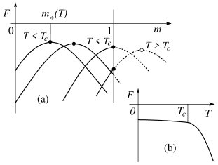
Figure 3: (a) Sketch of the free energy density $F(m,T)$ for a $m$-fold replicated system as a function of the replica parameter $m$ for different values of the temperature $T$. The smooth decrease of the maximum in $F(m)$ with increasing temperature $T$ reflects the (weak) temperature dependence of $f_{\mathrm{min}}(T)$. (b) Free energy density as a function of $T$ after eliminating the replica parameter $m$.

In summary, we can adopt the following strategy in order to obtain a proper thermodynamic description of the glass transition associated with an entropy crisis: First, we have to compute the free energy density $F(m,T)$ of the $m$-fold replicated system in the molecular liquid phase and for arbitrary values of the parameter $m$. Next, this function has to be analytically continued to arbitrary (non-integer) values of $m$, in particular, values within the interval $0<m<1$. In a last step, we have to find the maximum of the function $F(m,T)$ within the interval $[0,1]$. If the maximum of the replica free energy $F(m,T)$ is realized at $m_{*}(T)<1$ (i.e., $T<T_{c}$, cf. Fig. 3), we conclude that the original system (with $m=1$) is in the glass phase and its free energy density is given by $F_{\mathrm{glass}}=F[m_{*}(T),T]$. On the other hand, a maximum in $F(m,T)$ located at a value $m_{*}(T)>1$ (i.e., $T_{c}<T$) tells us that the original system resides in the liquid phase. The true free energy density of the original system with $m=1$ then is given by the value $F_{\mathrm{liquid}}=F(m=1,T)$ assumed at the border of the interval. Finally, the transition from one regime to the other at $m_{*}(T_{c})=1$ determines the transition temperature $T_{c}$.

II.3 Implementation of replica calculation

We consider a system of $N$ identical particles, confined within a macroscopic box of volume $V$ and described by the Hamiltonian $H[{\bf x}_{1},{\bf x}_{2},...,{\bf x}_{N}]\equiv H[{\bf x}]$. The partition function for $m$ uncoupled copies of this system reads

$$Z_{m}\!=\!\frac{1}{(N!)^{m}}\prod_{i=1}^{N}\prod_{a=1}^{m}\int\!\frac{d^{D}{\bf x}_{i}^{a}}{s^{D}}\exp\Bigl{[}-\!\beta\sum_{a=1}^{m}H[{\bf x}^{a}]\Bigr{]},$$ (9)

where $\beta=1/T$ denotes the inverse temperature and $s$ is the particle size (or the lattice spacing) which we set to unity hereafter, $s=1$. Also, we define the density $\rho=N/V$, which we keep constant in the thermodynamic limit, as well as the mean interparticle distance $L=\rho^{-1/D}$. The free energy density is given by the expression $F(m,\beta)=-({\rm ln}Z_{m})/m\beta N$. Following the above strategy, we assume that the spatial positions of the particles in different replicas are correlated, i.e., the particles arrange in ‘replica molecules’; technically this is implemented via a transformation to center of mass (${\bf x}_{i}$) and relative coordinates (${\bf u}_{i}^{a}$), ${\bf x}_{i}^{a}={\bf x}_{i}+{\bf u}_{i}^{a}$, and assuming that the displacements ${\bf u}_{i}^{a}$ remain bounded, $|{\bf u}_{i}^{a}|\ll L$. In addition, the coordinates have to satisfy the constraint

$$\sum_{a=1}^{m}{\bf u}_{i}^{a}=0.$$ (10)

Finally, the assumption that this replica system resides in the molecular liquid state implies that the molecular positions ${\bf x}_{i}$ take on arbitrary values within the entire system volume. Hence, the replicated partition function can be written in the form

$$Z_{m} = \frac{m^{DN}}{N!}\prod_{i=1}^{N}\prod_{a=1}^{m}\int d^{D}{\bf u}_{i}^{a}\,\delta\Bigl{(}\sum_{b=1}^{m}{\bf u}_{i}^{b}\Bigr{)}$$ (11)

$$\!\!\!\times\prod_{i=1}^{N}\int d^{D}{\bf x}_{i}\exp\Bigl{[}-\beta\sum_{a=1}^{m}H[{\bf x}+{\bf u}^{a}]\Bigr{]}.$$

Here, the additional factor $m^{DN}$ is due to the change of variables ${\bf x}_{i}^{a}={\bf x}_{i}+{\bf u}_{i}^{a}$ with the constraint (10).

Our problem now has assumed a form which is similar to the replica representation of usual glass problems with quenched disorder. The molecular coordinates ${\bf x}_{i}$ play the role of the disorder parameters, while the displacements ${\bf u}_{i}^{a}$ represent the dynamical variables. Our task then is to average over the disorder parameters $\{{\bf x}_{i}\}$ in order to arrive at the partition function $Z_{m}$ expressed through a new effective replica Hamiltonian $H_{m}[{\bf u}^{a}]$,

$$Z_{m}=\prod_{i=1}^{N}\prod_{a=1}^{m}\int d^{D}{\bf u}_{i}^{a}\,\delta\Bigl{(}\sum_{b=1}^{m}{\bf u}_{i}^{b}\Bigr{)}\exp\left(-\beta H_{m}[{\bf u}^{a}]\right),$$ (12)

where the replica variables ${\bf u}_{i}^{a}$ usually become coupled. The final integration over the dynamical variables ${\bf u}_{i}^{a}$ then will provide us with the free energy density $F(m,\beta)$. Note that in order to assure the consistency of the calculation, we have to compute the mean squared displacement amplitude $\langle{\bf u}^{2}\rangle^{1/2}$ and verify that it is indeed smaller than the average distance between the particles, $\langle{\bf u}^{2}\rangle^{1/2}\ll L$. The above program then is carried out for the specific interaction introduced in the next section.

II.4 Model interaction

We define the inter-particle interaction in the Hamiltonian (1) in terms of the spherically symmetric potential $U(|{\bf x}|)$ (cf. Fig. 1, we define $R_{\scriptscriptstyle\pm}=R\pm r_{0}$)

$$U(|{\bf x}|)\!=\!\!\left\{\begin{array}[]{ll}\displaystyle{\!\Bigl{[}\frac{(|{\bf x}|-R)^{2}}{r_{0}^{2}}-1\Bigr{]}},&R_{\scriptscriptstyle-}<|{\bf x}|<R_{\scriptscriptstyle+},\\ \vskip 5.0pt\cr 0,&\!\!|{\bf x}|\not\in\left[R_{\scriptscriptstyle-},R_{\scriptscriptstyle+}\right].\\ \end{array}\right.$$ (13)

We require the thickness $2r_{0}$ of the spherical attractive shell to be small compared to the radius $R$, $r_{0}\ll R$. At the same time, we choose a shell thickness $r_{0}$ large compared to the particle size, which we choose equal to unity for simplicity, ${r_{0}}\gg 1$; this allows us to perform all the calculations within the continuum limit. More specifically, we will treat the particles as point-like objects when integrating over positions. On the other hand, a proper hard core repulsion is required in order to inhibit the trivial collapse of the system into a pair of clusters separated by $R$ with $N/2$ particles each.

For later convenience we introduce the volume integral

$$\int d^{D}{\bf x}\,U(|{\bf x}|) = \int_{R_{\scriptscriptstyle-}\leq|{\bf x}|\leq R_{\scriptscriptstyle+}}\!\!\!\!\!\!\!\!\!\!\!\!\!\!\!\!\!\!\!\!d^{D}{\bf x}\quad\ \left[\frac{(|{\bf x}|-R)^{2}}{r_{0}^{2}}-1\right]$$ (14)

$$\simeq -V_{0}\sim R^{D-1}r_{0}$$

with $V_{0}=2r_{0}S_{D}$ the volume of a spherical shell with radius $R$ and width $2r_{0}$ (here, $S_{D}=2\pi^{D/2}$ $R^{(D-1)}/\Gamma(D/2)\sim R^{(D-1)}$ is the area of the $D$-dimensional sphere with radius $R$). Finally, we will assume a particle density near to that of the liquid/crystal phase by fixing the mean particle separation $L=\rho^{-1/D}$ close to the interaction radius $R$, $L\sim R$.

Simple geometric considerations tell that in addition to the low-energy crystal configuration (characterized by space periodicity and a fixed number of nearest neighbours), the present model also develops numerous metastable low-energy states with a disordered/glassy arrangement of particles. Such states are inhomogeneous in space and exhibit a notably smaller average number of nearest neighbours as compared to the crystal. Also, geometric considerations tell that such glassy configurations are ‘well separated’ from the ordered crystal: their transformation into the crystal state would require a global (on the scale of the entire system) rearrangement of the particles which would involve large energies. It is this type of random glass-like configurations which is at the focus of our further studies below.

III Replica free energy

We start from the expression (11) for the replica partition function in the form

$$Z_{m}=\frac{m^{DN}V^{N}}{N!}\prod_{i=1}^{N}\prod_{a=1}^{m}\int d^{D}{\bf u}_{i}^{a}\,\delta\Bigl{(}\sum_{b=1}^{m}{\bf u}_{i}^{b}\Bigr{)}$$ (15)

$$\times\!\prod_{i=1}^{N}\!\int\!\frac{d^{D}{\bf x}_{i}}{V}\exp\Bigl{\{}-\frac{\beta}{2}\sum_{a=1}^{m}\sum_{i,j=1}^{N}\!U\bigl{[}|({\bf x}_{i}\!-\!{\bf x}_{j})\!+\!{\bf u}_{ij}^{a}|\bigr{]}\!\Bigr{\}},$$

where ${\bf u}_{ij}^{a}\equiv({\bf u}_{i}^{a}-{\bf u}_{j}^{a})$. For large $N$, we can approximate $N!\sim N^{N}$ and obtain the prefactor $m^{DN}V^{N}/N!\simeq\exp[DN{\rm ln}(m)-N{\rm ln}(\rho)]$ with the density $\rho=N/V$. The replica partition function then takes the form

$$Z_{m}=e^{\left[DN{\rm ln}(m)-N{\rm ln}(\rho)\right]}\prod_{i=1}^{N}\prod_{a=1}^{m}\int d^{D}{\bf u}_{i}^{a}\,\delta\Bigl{(}\sum_{b=1}^{m}{\bf u}_{i}^{b}\Bigr{)}$$

$$\qquad\qquad\qquad\qquad\times\bigl{\langle}\exp\left(-\beta H\left[{\bf x};{\bf u}\right]\right)\bigr{\rangle}_{{\bf x}}$$ (16)

with the average over positions

$$\langle\Phi\left[{\bf x}_{1},\dots,{\bf x}_{N}\right]\rangle_{{\bf x}}\equiv\prod_{i=1}^{N}\int\frac{d^{D}{\bf x}_{i}}{V}\Phi\left[{\bf x}_{1},\dots,{\bf x}_{N}\right].$$ (17)

The average of the exponential in Eq. (III) can be calculated with the help of a cumulant expansion,

$$\bigl{\langle}\exp\left(-\beta H\left[{\bf x};{\bf u}\right]\right)\bigr{\rangle}_{\bf x}$$ (18)

$$\simeq\exp\Bigl{[}-\beta\langle H\rangle_{\bf x}+\frac{\beta^{2}}{2!}\beta^{2}\langle\langle H^{2}\rangle\rangle_{\bf x}-\frac{\beta^{3}}{3!}\langle\langle H^{3}\rangle\rangle_{\bf x}+\;...\;\Bigr{]},$$

where $\langle\langle H^{k}\rangle\rangle_{\bf x}$ denotes the $k$-th cumulant of the Hamiltonian; in particular,

$$\langle\langle H^{2}\rangle\rangle_{\bf x} \equiv \langle H^{2}\rangle_{\bf x}-\langle H\rangle_{\bf x}^{2},$$ (19)

$$\langle\langle H^{3}\rangle\rangle_{\bf x} \equiv \langle H^{3}\rangle_{\bf x}-3\langle H^{2}\rangle_{\bf x}\langle H\rangle_{\bf x}+2\langle H\rangle_{\bf x}^{2}.$$ (20)

III.1 First- and second-order contributions

Using the potential (13) with its volume integral (14), we find the first-order term

$$\langle H\rangle_{\bf x}\! = \!\frac{1}{2}\sum_{a=1}^{m}\sum_{i,j=1}^{N}\langle U\left[|({\bf x}_{i}-{\bf x}_{j})+{\bf u}_{ij}^{a}|\right]\rangle_{\bf x}$$

$$= \!\frac{N^{2}}{2}m\int\frac{d^{D}{\bf x}}{V}U\left(|{\bf x}|\right)\simeq-\frac{N\rho V_{0}}{2}m.$$

For the second-order cumulant (see Fig. 4(a) for a diagrammatic representation), we find

$$\langle\langle H^{2}\rangle\rangle_{\bf x}=\frac{1}{4}\sum_{a,b=1}^{m}\sum_{i,j,k,l}^{N}\langle\langle U[|({\bf x}_{i}-{\bf x}_{j})+{\bf u}_{ij}^{a}|]$$

$$\qquad\qquad\times U[|({\bf x}_{k}-{\bf x}_{l})+{\bf u}_{kl}^{b}|]\rangle\rangle_{\bf x_{i},x_{i},x_{j},x_{k}}.$$ (22)

Only correlated positions $(i,j)=(k,l)$ (i.e., connected graphs) give a finite contribution (since $\langle U(|\delta{\bf x}_{ij}+{\bf u}_{ij}^{b}|)U(|\delta{\bf x}_{kl}+{\bf u}_{kl}^{b}|)\rangle=\langle U(|{\bf x}|)\rangle\langle U(|{\bf x}|)\rangle$), hence

$$\langle\langle H^{2}\rangle\rangle_{\bf x} = \frac{1}{2}\sum_{a,b=1}^{m}\sum_{i,j}^{N}\int\frac{d^{D}{\bf x}}{V}$$ (23)

$$\times\,U\left(|{\bf x}+{\bf u}_{ij}^{a}|\right)\,U\left(|{\bf x}+{\bf u}_{ij}^{b}|\right).$$

Figure 4: Diagrammatic representation of the second-order cumulant; (a) only connected graphs give a finite contribution, (b) contributions after expansion in the displacement ${\bf u}_{ij}^{a}$.

We assume that typical deviations $\langle|{\bf u}|^{2}\rangle^{1/2}$ are small compared to $r_{0}$ (this assumption has to be verified at the end of the calculation), allowing us to expand the potential $U[|({\bf x}+{\bf u}_{ij}^{a}|]$ in the displacement ${\bf u}_{ij}^{a}$,

$$\sum_{a=1}^{m}U(|({\bf x}+{\bf u}_{ij}^{a}|)\simeq mU(|{\bf x}|)+\sum_{\alpha=1}^{D}U_{\alpha}^{\prime}(|{\bf x}|)\sum_{a=1}^{m}u_{ij(\alpha)}^{a}$$

$$\qquad\qquad+\frac{1}{2}\sum_{\alpha\beta=1}^{D}U_{\alpha\beta}^{\prime\prime}(|{\bf x}|)\sum_{a=1}^{m}u_{ij(\alpha)}^{a}u_{ij(\beta)}^{a}.$$ (24)

Here, the indices $\alpha,\beta$ denote spatial vector components and $U_{\alpha}^{\prime}$, $U_{\alpha\beta}^{\prime\prime}$ are corresponding derivatives. The expansion (III.1) involves the small parameter $u^{2}/r_{0}^{2}$, allowing its termination at the second order, cf. Fig. 4(b) for a diagrammatic representation. Its second term (linear in $u$) vanishes due to the constraint (10) and we arrive at the expression

$$\langle\langle H^{2}\rangle\rangle_{\bf x}\simeq\frac{N^{2}}{2}m^{2}\langle U^{2}(|{\bf x}|)\rangle_{\bf x}$$ (25)

$$+\frac{1}{2}m\sum_{\alpha\beta=1}^{D}\langle U(|{\bf x}|)U_{\alpha\beta}^{\prime\prime}(|{\bf x}|)\rangle_{\bf x}\sum_{a=1}^{m}\sum_{i,j,}^{N}u_{ij(\alpha)}^{a}u_{ij(\beta)}^{a}.$$

Using the definition of the potential $U(|{\bf x}|)$, Eq. (13), we obtain

$$U_{\alpha\beta}^{\prime\prime}(R_{\scriptscriptstyle-}\!<\!|{\bf x}|\!<\!R_{\scriptscriptstyle+})\!=\!\frac{2}{r_{0}^{2}}\Bigl{[}\delta_{\alpha\beta}\Bigl{(}\!1-\frac{R}{|{\bf x}|}\Bigr{)}+n_{\alpha}n_{\beta}\frac{R}{|{\bf x}|}\Bigr{]},$$ (26)

and 0 else, where $n_{\alpha}=x_{\alpha}/|{\bf x}|$ is the unit vector in the direction of ${\bf x}$. Accounting for the smallness of $r_{0}$, $r_{0}\ll R$, we find the positional averages

$$\langle U(|{\bf x}|)^{2}\rangle_{\bf x} \equiv \int\frac{d^{D}{\bf x}}{V}\bigl{[}U(|{\bf x}|)\bigr{]}^{2}\simeq\frac{V_{0}}{V},$$ (27)

$$\langle U(|{\bf x}|)U_{\alpha\beta}^{\prime\prime}(|{\bf x}|)\rangle_{\bf x} \equiv \int\frac{d^{D}{\bf x}}{V}U(|{\bf x}|)U_{\alpha\beta}^{\prime\prime}(|{\bf x}|)$$

$$\simeq -\frac{V_{0}}{V}\frac{2}{r_{0}^{2}}\langle n_{\alpha}n_{\beta}\rangle=-\frac{V_{0}}{V}\frac{2}{r_{0}^{2}D}\delta_{\alpha\beta},$$

and substituting these results back into Eq. (25) we obtain

$$\langle\langle H^{2}\rangle\rangle_{\bf x} \simeq \frac{N\rho V_{0}}{2}m^{2}$$

$$- \frac{N\rho V_{0}}{Dr_{0}^{2}}m\sum_{i,j}^{N}\sum_{\alpha=1}^{D}\sum_{a=1}^{m}\bigl{[}u_{ij(\alpha)}^{a}\bigr{]}^{2}.$$

Going back to the original displacement coordinates ${\bf u}_{i}^{a}$ and accounting for the restrictions (the second condition corresponds to a global shift of all particles in the system) $\sum_{a=1}^{m}{\bf u}_{i}^{a}=0$ and $\sum_{i}^{N}{\bf u}_{i}^{a}=0$, we obtain the following contribution from the first- and second-order cumulants,

$$-\beta\langle H\rangle_{\bf x}+\frac{\beta^{2}}{2!}\langle\langle H^{2}\rangle\rangle_{\bf x}$$ (30)

$$\qquad\qquad\qquad\simeq\frac{N\rho V_{0}}{2}\Bigl{[}(\beta m)+\frac{1}{2!}(\beta m)^{2}\Bigr{]}$$

$$\qquad\qquad\qquad-\frac{\rho V_{0}\beta}{Dr_{0}^{2}}(\beta m)\sum_{\alpha=1}^{D}\sum_{a=1}^{m}\sum_{i}^{N}\bigl{[}u_{i(\alpha)}^{a}\bigr{]}^{2}.$$

III.2 Third-order cumulant

Next, we determine the contributions from the third-order cumulant $\langle\langle H^{3}\rangle\rangle_{\bf x}\equiv(\Xi/2+2\Delta)$ which contributes with two terms describing two-point ($\Xi$) and three-point ($\Delta$) correlations. These correspond to the connected diagrams shown in Fig. 5(a) and can be written in the form

$$\Xi=\sum_{a,b,c=1}^{m}\sum_{i,j}^{N}\langle U[|{\bf x}+{\bf u}_{ij}^{a}|]U[|{\bf x}+{\bf u}_{ij}^{b}|]U[|{\bf x}+{\bf u}_{ij}^{c}|]\rangle_{\bf x}$$ (31)

and

$$\Delta=\sum_{a,b,c=1}^{m}\sum_{i,j,k}^{N}\langle U[|({\bf x}_{i}-{\bf x}_{j})+{\bf u}_{ij}^{a}|]$$ (32)

$$\quad\times U[|({\bf x}_{j}-{\bf x}_{k})+{\bf u}_{jk}^{b}|]U[|({\bf x}_{k}-{\bf x}_{i})+{\bf u}_{ki}^{c}|]\rangle_{{\bf x}_{i}{\bf x}_{j}{\bf x}_{k}}.$$

Figure 5: Diagrams contributing to third order in the interaction potential: (a) two-point and three-point (loop) diagrams, (b) contribution of the two-point diagram after expansion in the displacement ${\bf u}$, (c) contribution of the three-point diagram after expansion in the displacement ${\bf u}$.

Expanding the two-point contribution Eq. (31) in the displacement ${\bf u}$ and integrating over ${\bf x}$, we obtain up to second order in the displacement ${\bf u}$ (cf. Fig. 5(b))

$$\Xi=-N\rho V_{0}m^{3}+\frac{6\rho V_{0}}{Dr_{0}^{2}}m^{2}\sum_{\alpha=1}^{D}\sum_{a=1}^{m}\sum_{i}^{N}\bigl{[}u_{i(\alpha)}^{a}\bigr{]}^{2}\!\!.$$ (33)

Next, we concentrate on the three-point (loop) contribution and first simplify the expression by redefining the coordinates ${\bf x}_{i},{\bf x}_{j}$, ${\bf x}_{k}$,

$$\Delta=\sum_{a,b,c=1}^{m}\sum_{i,j,k}^{N}\langle U[|{\bf x}_{1}+{\bf u}_{ij}^{a}|]$$ (34)

$$\qquad\qquad\times U[|{\bf x}_{2}+{\bf u}_{jk}^{b}|]U[|{\bf x}_{1}-{\bf x}_{2}+{\bf u}_{ik}^{c}|]\rangle_{{\bf x}_{1}{\bf x}_{2}}.$$

We expand in the displacement ${\bf u}$, cf. Fig. 5(c), and arrive at the expression

$$\Delta=N^{3}m^{3}\langle U(|{\bf x}_{1}|)U(|{\bf x}_{2}|)U(|{\bf x}_{1}-{\bf x}_{2}|)\rangle_{{\bf x}_{1}{\bf x}_{2}}$$ (35)

$$+\frac{3N}{2}m^{2}\sum_{\alpha\beta=1}^{D}\langle U(|{\bf x}_{1}|)U(|{\bf x}_{2}|)U_{\alpha\beta}^{\prime\prime}(|{\bf x}_{1}-{\bf x}_{2}|)\rangle_{{\bf x}_{1}{\bf x}_{2}}$$

$$\qquad\qquad\qquad\qquad\qquad\qquad\times\sum_{a=1}^{m}\sum_{ij}^{N}u_{ij(\alpha)}^{a}u_{ij(\beta)}^{a}.$$

Using the definition (13) of the potential and its derivatives (26), we find for the above disorder averages (again assuming that $r_{0}\ll R$)

$$\langle U(|{\bf x}_{1}|)U(|{\bf x}_{2}|)U(|{\bf x}_{1}-{\bf x}_{2}|)\rangle_{{\bf x}_{1},{\bf x}_{2}}\simeq-\frac{V_{0}V_{1}}{V^{2}},$$ (36)

$$\langle U(|{\bf x}_{1}|)U(|{\bf x}_{2}|)U_{\alpha\beta}^{\prime\prime}(|{\bf x}_{1}-{\bf x}_{2}|)\rangle_{{\bf x}_{1},{\bf x}_{2}}\simeq\delta_{\alpha\beta}\frac{2}{r_{0}^{2}D}\frac{V_{0}V_{1}}{V^{2}},$$

with $V_{1}\sim R^{D-2}r_{0}^{2}$ the intersection volume of two spherical shells with radius $R$ and width $r_{0}$; the three-point contribution then takes the form

$$\Delta = -N\rho^{2}V_{0}V_{1}m^{3}$$

$$\qquad\qquad+\frac{6\rho^{2}V_{0}V_{1}}{Dr_{0}^{2}}m^{2}\sum_{\alpha=1}^{D}\sum_{a=1}^{m}\sum_{i}^{N}\bigl{[}u_{i(\alpha)}^{a}\bigr{]}^{2}.$$

Replacing the density $\rho$ with the distance parameter $L$ and assuming that $R\leq L$, we find that the three-point contribution is reduced with respect to the two-point term (33) by the small factor

$$\rho V_{1}\sim L^{-D}R^{D-2}r_{0}^{2}=\left(\frac{R}{L}\right)^{D}\left(\frac{r_{0}}{R}\right)^{2}\ll 1.$$ (38)

III.3 k-th-order cumulants

Comparing the magnitude of the above diagrams, we note that all two-point terms (cf. Fig. 6) appear with similar weight and we have to resum them; the two-point part of the $k$-th-order cumulant contributes with a term $(-\beta)^{k}\langle\langle H^{k}\rangle\rangle_{2\rm pt}/k!$ where ($k\geq 2$, see (III.1) for the $k=1$ contribution)

$$(-1)^{k}\langle\langle H^{k}\rangle\rangle_{2\rm pt}\! \simeq \!\frac{N\rho V_{0}}{2}m^{k}$$

$$- \!\frac{k\rho V_{0}}{Dr_{0}^{2}}m^{k-1}\sum_{\alpha=1}^{D}\sum_{a=1}^{m}\sum_{i}^{N}\bigl{[}u_{i(\alpha)}^{a}\bigr{]}^{2}.$$

Figure 6: Diagrammatic representation of the two-point contribution to the $k$-th-order cumulant after expansion in the displacement ${\bf u}$.

On the other hand, the loop diagrams remain small: a simple geometrical analysis shows that each $k$-th-order loop involves an additional small factor of order ($k\geq 3$)

$$(\rho V_{0})^{k-3}(\rho V_{1}) \sim \biggl{[}\Bigl{(}\frac{R}{L}\Bigr{)}^{D}\Bigl{(}\frac{r_{0}}{R}\Bigr{)}\biggr{]}^{k-3}\left(\frac{R}{L}\right)^{D}\left(\frac{r_{0}}{R}\right)^{2}$$ (40)

$$= \left(\frac{R}{L}\right)^{D(k-2)}\left(\frac{r_{0}}{R}\right)^{k-1}\ll 1.$$

Thus, we conclude that for the present model with properly chosen parameters $r_{0}\ll R$ and $R\leq L$ all loop-type contributions produce only small corrections as compared to the main terms arising from the two-point diagrams.

It remains to sum up the two-point contributions, which corresponds to the substitution $[\beta m+(\beta m)^{2}/2!+(\beta m)^{3}/3!\dots\rightarrow[\exp(\beta m)-1]$, and we obtain the partition function averaged over disorder in the form

$$Z_{m}\! = \!\exp\bigl{\{}DN{\rm ln}(m)\!-\!N{\rm ln}(\rho)\!+\!(N\rho V_{0}/2)\bigl{[}e^{\beta m}\!-\!1\bigr{]}\bigr{\}}$$

$$\times \prod_{i=1}^{N}\prod_{\alpha=1}^{D}\biggl{\{}\prod_{a=1}^{m}\int d^{D}u_{i(\alpha)}^{a}\,\delta\Bigl{(}\sum_{b=1}^{m}u_{i(\alpha)}^{b}\Bigr{)}$$

$$\times \exp\biggl{[}-\frac{\rho V_{0}\beta}{Dr_{0}^{2}}\bigl{[}e^{\beta m}-1\bigr{]}\sum_{a=1}^{m}\Bigl{[}u_{i(\alpha)}^{a}\Bigr{]}^{2}\biggr{]}\biggr{\}}.$$

A simple Gaussian integration over the displacements $u_{i(\alpha)}^{a}$ then results in the expression

$$Z_{m}\! = \!\exp\biggl{\{}\frac{DN}{2}{\rm ln}(m)-N{\rm ln}(\rho)+\frac{N\rho V_{0}}{2}\bigl{[}e^{\beta m}-1\bigr{]}$$ (42)

$$- \frac{ND(m-1)}{2}{\rm ln}\Bigl{[}\frac{\rho V_{0}\beta}{Dr_{0}^{2}}\bigl{[}e^{\beta m}-1\bigr{]}\Bigr{]}\biggr{\}}$$

and taking the logarithm we obtain (after rearranging terms) the replica free energy density $F(m,\beta)=-(1/N\beta m){\rm ln}\left(Z_{m}\right)$ in the form,

$$F(m,\beta)=F_{0}(\beta)-\frac{\rho V_{0}}{2\beta m}\bigl{[}e^{\beta m}-1\bigr{]}$$ (43)

$$\quad-\frac{D}{2\beta m}\Bigl{\{}{\rm ln}\Bigl{[}\frac{\rho V_{0}L^{2}\beta m}{Dr_{0}^{2}}\Bigr{]}-(m-1){\rm ln}\bigl{[}e^{\beta m}-1\bigr{]}\Bigr{\}},$$

where we have separated the term

$$F_{0}(\beta)=\frac{D}{2\beta}{\rm ln}\left[\frac{\rho V_{0}\beta}{Dr_{0}^{2}}\right]$$ (44)

which does not depend on the replica number $m$. When proceeding with (43) we have to keep in mind two restrictions which are limiting its validity: i) our continuum approximation prevents us from reaching very low temperatures, and ii) the smallness of the mean square displacements $\langle u^{2}\rangle\ll r_{0}^{2}$ requires a sufficiently large parameter $\beta m$ or a sufficiently small temperature $T$. We proceed with a detailed analysis of these restrictions.

III.4 Restrictions

In order to justify the continuum limit in the integrations over the displacements $u_{i(\alpha)}^{a}$, cf. Eq. (III.3), where we assume that $|u_{i(\alpha)}^{a}|\gg 1$, we have to demand that the width

$$\frac{\rho V_{0}\beta}{Dr_{0}^{2}}\bigl{[}e^{\beta m}-1\bigr{]}\ll 1.$$ (45)

Hence, the application of the continuuum limit puts a lower limit on the system temperature, or, alternatively, on the largeness of the replica parameter $m$. We will return to this point in the next section.

The second restriction derives from the condition that typical values of the displacements $u_{i(\alpha)}^{a}$ as defined by the Boltzmann weight in Eq. (III.3) should be small on the scale of the width $r_{0}$ of the attractive shell; the Gaussian integration then yields the condition

$$\langle u^{2}\rangle\equiv\frac{1}{m}\sum_{a=1}^{m}\bigl{\langle}[u^{a}]^{2}\bigr{\rangle}\sim\frac{Dr_{0}^{2}/\rho V_{0}}{\beta m[\exp(\beta m)-1]}\ll r_{0}^{2}.$$

Since $\rho V_{0}\sim(R/L)^{D}(r_{0}/R)\ll 1$ for $R\leq L$, we can conclude that the result for the replica free energy density describing the molecular liquid state is valid if $\beta m$ is sufficiently large and bounded by the condition

$$\rho V_{0}\,\beta m\exp\left(\beta m\right)\gg 1.$$ (46)

The violation of this condition implies that the particles, originally assumed to be bounded in ‘replica molecules’, would escape from the potential well $U(|{\bf x}|)$ and become effectively decoupled. In this situation the state of our replica system would not correspond to the molecular liquid phase any more and the above analysis cannot be applied. The same conclusion also follows from our general qualitative arguments in Sec. II.B: the limit of small replica parameter $m$ corresponds to a high effective temperature of the replicated system where no ‘replica molecules’ could survive.

IV Results and conclusions

IV.1 Free energy density and $T_{c}$

Let us return to the free energy density (43) and determine the replica parameter $m$. Assuming that $\exp\left(\beta m\right)\gg 1$, we first simplify the function $F(m,\beta)$,

$$F(m,\beta) \simeq F_{0}(\beta)-\frac{\rho V_{0}}{2\beta m}e^{\beta m}-\frac{D}{2\beta m}{\rm ln}\biggl{[}\frac{\rho V_{0}L^{2}\beta m}{Dr_{0}^{2}}\biggr{]}$$ (47)

$$\qquad\qquad\qquad+D(m-1)/2,$$

and find its maximum in the replica parameter $m$ from the condition $\partial_{m}F(m,\beta)=0$,

$$\frac{\rho V_{0}}{D}\left(\beta m-1\right)e^{\beta m}-\Bigl{(}\beta m^{2}-1\Bigr{)}={\rm ln}\biggl{[}\frac{\rho V_{0}L^{2}\beta m}{Dr_{0}^{2}}\biggr{]}.$$ (48)

With the parameters $r_{0}/L,\,\rho V_{0}\ll 1$ and $\rho V_{0}L^{2}/r_{0}^{2}\gg 1$, the above equation assumes the solution (to logarithmic accuracy)

$$\beta m_{*}(\beta)\simeq{\rm ln}\frac{D}{\rho V_{0}}\!+\!{\rm ln}\biggl{[}\frac{{\rm ln}(\rho V_{0}L^{2}/eDr_{0}^{2})}{{\rm ln}(D/\rho V_{0})}+\frac{1}{\beta}{\rm ln}\frac{D}{\rho V_{0}}\biggr{]}.$$ (49)

In the following, we concentrate on the case of matching density $\rho\sim R^{-D}$, i.e., $L\sim R$, and substituting $\rho\sim R^{-D}$, $V_{0}\sim R^{D-1}r_{0}$ we easily verify that the above conditions are satisfied,

$$\rho V_{0} \sim \left(\frac{R}{L}\right)^{D}\frac{r_{0}}{R}\sim\frac{r_{0}}{R}\ll 1,$$ (50)

$$\rho V_{0}\frac{L^{2}}{r_{0}^{2}} \sim \left(\frac{R}{L}\right)^{D-1}\frac{L}{r_{0}}\sim\frac{R}{r_{0}}\gg 1.$$ (51)

The solution $m_{*}$ then assumes the simplified form

$$\beta m_{*}(\beta)\sim{\rm ln}\frac{DR}{r_{0}}+{\rm ln}\Bigl{(}1+\frac{1}{\beta}{\rm ln}\frac{DR}{r_{0}}\Bigr{)}.$$ (52)

The transition temperature $T_{c}$ is defined by the condition $m_{*}(\beta_{c})=1$ (see Sec. II.B) and we arrive at the estimate,

$$T_{c}\sim\frac{1}{{\rm ln}(DR/r_{0})}\ll 1.$$ (53)

Next, we should verify that the above conditions (45) and (46) are satisfied; they can be cast into the form

$$1\ll\frac{r_{0}}{R}\beta m\,e^{\beta m}\ll mDr_{0}^{2};$$ (54)

with

$$\beta m>\beta m_{*}(T)\sim{\rm ln}(DR/r_{0}).$$ (55)

The first relation (guaranteeing a small displacement amplitude $\langle u^{2}\rangle\ll r_{0}^{2}$) is satisfied within the entire low-temperature phase $0\leq T\leq T_{c}$. The second relation (allowing us to make use of the continuum limit) implies that $T\gg 1/r_{0}^{2}$. This condition is satisfied at $T_{c}$ since $\ln(DR/r_{0})\ll r_{0}^{2}$ for sufficiently large $r_{0}$; however, it is violated at low temperatures $T\sim 1/r_{0}^{2}$, thus limiting the applicability of our results to sufficiently high values of $T$.

The logarithmic dependence of $T_{c}$ found above can be easily understood from an order of magnitude estimate of the free energies of the liquid and glass phase. Let us assume that the average number of particles interacting in the frozen state is of the order of $D$ (see below, Eqs. (73) and (74)). Then each particle contributes with an energy $-D$ to the free energy of the system. Second, the freezing into the glass state confines the particle to the volume $r_{0}^{D}$ which is small with respect to the volume $R^{D}$ available in the liquid state. This produces a deficit $\ln(R^{D}/r_{0}^{D})$ in the entropy of the frozen state as compared to the liquid. The difference in the free energies between the frozen and liquid states then can be estimated as $\Delta F\sim-D+T\ln(R^{D}/r_{0}^{D})$; this quantity turns negative at temperatures $T<T_{c}\sim[\ln(R/r_{0})]^{-1}$ and the frozen state becomes preferable.

An independent confirmation of the result (53) can be obtained from a virial expansion LL : to third order the equation of state takes the form

$$\frac{pV}{NT}=1+B(T)\frac{N}{V}+C(T)\frac{N^{2}}{V^{2}}+\dots$$ (56)

with the coefficients

$$B(T) = -\frac{1}{2}\int d^{3}x\,f({\bf x}),$$ (57)

$$C(T) = -\frac{1}{3}\int d^{3}x_{1}d^{3}x_{2}\,f({\bf x}_{1})f({\bf x}_{2})f({\bf x}_{1}-{\bf x}_{2}),$$

and $f({\bf x})=\exp[-\beta U({\bf x})]-1$. Inserting the expression (13) for the potential $U$ we can rewrite

$$f({\bf x})\simeq\left\{\begin{array}[]{ll}\exp(\beta),&R_{\scriptscriptstyle-}<|{\bf x}|<R_{\scriptscriptstyle+},\\ \vskip 3.0pt\cr 0,&|{\bf x}|\not\in[R_{\scriptscriptstyle-},R_{\scriptscriptstyle+}],\\ \end{array}\right.$$ (58)

and using the results (14) and (36) above, we find $B\simeq-R^{D}(r_{0}/R)\exp(\beta)$ and $C(T)\simeq-R^{2D}(r_{0}/R)^{3}\exp(3\beta)$. Assuming a high particle density with $L\sim R$, we find that the virial expansion diverges when $(r_{0}/R)\exp(\beta)\sim 1$, thus reproducing the critical temperature (53).

IV.2 Configurational entropy

We can use our free energy expression $F(m,\beta)$ to construct the form of the configurational entropy $S(f,T)$, cf. Fig. 1. Taking the derivative of the free energy $F(m,T)=f(m,T)-(T/m)S[f(m,T),T]$ and of $mF(m,T)$ with respect to $m$ and using that $\partial_{f}S=m/T$, cf. (7) and (8), we obtain the relations

$$\frac{m^{2}}{T}\partial_{m}F(m,T)=S(m,T),$$ (59)

$$\partial_{m}[mF(m,T)]=f(m,T),$$ (60)

and eliminating the parameter $m$, we arrive at an expression for $S(f,T)$. We use the free energy (43) in the limit of large $\beta m$ and expand (to third order in $m-m_{*}$) around the maximum $F(m_{*}(T),T)$. Expressing $m-m_{*}$ through $f-f_{\mathrm{min}}$ (with $f_{\mathrm{min}}=F(m_{*}(T),T)$) we find that the configurational entropy near $f_{\mathrm{min}}$ assumes the form

$$S(f,T)\approx\beta m_{*}(f-f_{\mathrm{min}})-\frac{2R}{r_{0}T}e^{-\beta m_{*}}(f-f_{\mathrm{min}})^{2}.$$ (61)

This result exhibits the shape expected for a configurational entropy triggering an entropy crisis as discussed in Sec. II.B, see Fig. 2.

IV.3 Order parameter

The above formal replica computations have been performed along the lines outlined in section II and fit well the original physical ideas regarding the nature of the liquid-glass phase transition. In order to describe the phase transition in more quantitative terms one has to introduce a properly defined order parameter which should be a measureable quantity, e.g., in computer simulations. Such an order parameter is easily defined if we exploit the replication trick where we have introduced $m$ identical copies of the same system. Let us assume that all these systems are allowed to thermalize independently but with the same (random) starting positions of the particles. If, at sufficiently high temperatures, the thermodynamic state of the system is a liquid, we expect the spatial positions of the particles belonging to different systems to be uncorrelated. On the other hand, if the thermodynamic state of the system is a frozen glass with each particle localized in a limited part of space, then the positions of the particles belonging to different replicas remain correlated, although the systems are uncoupled. Keeping in mind this qualitative scenario, we introduce the correlator

$$G=\frac{1}{N}\sum_{i=1}^{N}\bigl{\langle}\bigl{(}{\bf x}^{\scriptscriptstyle(1)}_{i}-{\bf x}^{\scriptscriptstyle(2)}_{i}\bigr{)}^{2}\bigr{\rangle},$$ (62)

where ${\bf x}^{\scriptscriptstyle(1)}_{i}$ is the position of the $i$-th particle in the system number 1, and ${\bf x}^{\scriptscriptstyle(2)}_{i}$ is the corresponding position (again of the $i$-th particle) of the system number 2. If the thermodynamic state of the system is a liquid, then the value of $G$ is proportional to $N^{-1}\sum_{i=1}^{N}\bigl{\langle}\bigl{(}{\bf x}^{\scriptscriptstyle(1)}_{i}\bigr{)}^{2}\bigr{\rangle}$, which is of the order of the linear size squared of the system and becomes infinite in the thermodynamic limit.

On the other hand, if the system is in the glass state, the situation is very different. In this case both ${\bf x}^{\scriptscriptstyle(1)}_{i}$ and ${\bf x}^{\scriptscriptstyle(2)}_{i}$ are localised near the same equilibrium positions and $G$ remains finite. Since all $m$ systems (replicas) considered here are equivalent, it is convenient to write the correlator (62) in the symmetric way

$$G=\frac{1}{N}\sum_{i=1}^{N}\frac{1}{m(m-1)}\sum_{a,b=1}^{m}\bigl{\langle}\bigl{(}{\bf x}^{\scriptscriptstyle(a)}_{i}-{\bf x}^{\scriptscriptstyle(b)}_{i}\bigr{)}^{2}\bigr{\rangle}.$$

We compute $G$ in the glass phase following the procedure described in section II and implemented in section III. Changing variables according to ${\bf x}_{i}^{a}={\bf x}_{i}+{\bf u}_{i}^{a}$, we find

$$G = \frac{1}{m(m\!-\!1)}\!\sum_{a,b=1}^{m}\!\bigl{\langle}\bigl{(}{\bf u}^{a}-{\bf u}^{b}\bigr{)}^{2}\bigr{\rangle}$$ (63)

$$= \frac{2Dm}{(m-1)}\bigl{\langle}\left(u^{a}_{\alpha}\right)^{2}\bigr{\rangle},$$

with the distribution of displacements $u^{a}_{\alpha}$ given by Eq. (III.3). A simple Gaussian integration yields

$$G\simeq T\frac{Dr_{0}^{2}}{\rho V_{0}}e^{-\beta m_{*}(T)},$$ (64)

where $\rho V_{0}\sim r_{0}/R$ (see Eq. (50)) and the value of $m_{*}(T)$ is given by the saddle-point solution $\beta m_{*}(T)\sim{\rm ln}\left(DR/r_{0}\right)$. Thus, in the glassy phase we find the finite value

$$G\simeq Tr_{0}^{2}.$$ (65)

We then define the order parameter $Q=(1+G)^{-1}$ assuming a finite value in the glassy phase and vanishing in the liquid,

$$Q=\left\{\begin{array}[]{ll}0,&\mbox{in the liquid, at}\;T>T_{c},\\ \vskip 5.0pt\cr\displaystyle{\frac{1}{1+Tr_{0}^{2}}},&\mbox{in the glass, at}\;T<T_{c},\end{array}\right.$$ (66)

where the transition temperature $T_{c}$ is given by Eq. (53). Note that the value of $Q$ remains finite at $T=T_{c}$, as expected for a phase transition driven by an entropy crisis. On the one hand, the physical order parameter describing this phase transition exhibits a finite jump at $T_{c}$ (as expected for a first-order phase transition), while, on the other hand, the free energy of the system is continuous in the transition point (with a continuous derivative as in a second-order transition). On a qualitative level this is easily understood: in the present approach the glass phase is characterized by the typical size of spatial cells where the particles remain localized. This volume is small in the low-temperature limit and grows with increasing temperature. At the transition to the liquid, the localization length is of the order of the interparticle distance and thus remains finite. Beyond the transition the particles move freely in the liquid phase and the localization length is infinite. Hence the transition resembles the usual solid-liquid transition, however, with the jump in entropy (latent heat) replaced by the entropy crisis scenario, guaranteeing the smooth transition in the free energy density.

IV.4 Free energy and entropy densities

Finally, we analyze in some more detail the value of the free energy- and entropy densities of the liquid and glassy phases. The free energy density $F(m,\beta)$ of the liquid derives from the result (43) with the replica parameter $m=1$ (we assume that $\beta\gg 1$ and choose $L\sim R$),

$$F_{\mathrm{liquid}}(\beta)\simeq-\frac{D}{2\beta}{\rm ln}(R^{2})-\frac{r_{0}}{2R\beta}e^{\beta};$$ (67)

the entropy density is given by the derivative

$$S_{\mathrm{liquid}}(\beta) = \beta^{2}\partial_{\beta}F_{\mathrm{liquid}}$$

$$\simeq D{\rm ln}R-\frac{r_{0}}{2R}(\beta-1)e^{\beta}.$$

We observe that at sufficiently low temperatures the entropy density of the liquid would become negative. Formally, this takes place at $\beta>\beta_{c}$ with $\beta_{c}$ defined by the condition

$$(\beta_{c}-1)e^{\beta_{c}}=\frac{DR}{r_{0}}{\rm ln}(R^{2}).$$ (69)

This negative entropy then signals the presence of the glass (or entropy crisis) transition: with $r_{0}/R\ll 1$ we obtain an estimate for the transition temperature,

$$\beta_{c}\sim{\rm ln}\frac{DR}{r_{0}},$$ (70)

which is in agreement with the analytic result (53).

The above arguments do not imply that the entropy of the liquid at the phase transition is equal to zero. In fact, as we shall see below, the phase transition into the glassy phase takes place before the entropy becomes zero. The above consideration of the liquid entropy is merely a qualitative estimate of the temperature below which we would run into trouble if we were to use the result (67).

Turning to the frozen state, we first discuss the situation deep in the glassy phase. The free energy density at $\beta\gg\beta_{c}$ follows from the result (47) with $m=m_{*}(\beta)$ defined by (52). Assuming $L\sim R$ we find the simplified expression

$$F_{\mathrm{glass}} \simeq -\frac{D}{2}\biggl{[}2+\Bigl{(}1-\frac{1}{\beta}\Bigr{)}\frac{{\rm ln}{\rm ln}(DR/r_{0})}{{\rm ln}(DR/r_{0})}$$ (71)

$$\qquad\qquad+\frac{1}{\beta}{\rm ln}\frac{r_{0}^{2}}{\beta}\biggr{]}.$$

Taking the derivative with respect to temperature we obtain the entropy density of the glassy phase,

$$S_{\mathrm{glass}}(\beta) = \beta^{2}\partial_{\beta}F_{\mathrm{glass}}$$

$$\simeq \frac{D}{2}\left[1+{\rm ln}\frac{r_{0}^{2}}{\beta}-\frac{{\rm ln}{\rm ln}(DR/r_{0})}{{\rm ln}(DR/r_{0})}\right].$$

Combining the results for the free energy and the entropy, we can derive an expression for the average energy per particle in the glassy phase which scales with the dimension $D$,

$$E=F_{\mathrm{glass}}+TS_{\mathrm{glass}}\simeq-A\,D;$$ (73)

the prefactor $A$ assumes a value close to unity,

$$A\simeq 1+\frac{{\rm ln}{\rm ln}(DR/r_{0})}{2{\rm ln}(DR/r_{0})}>1.$$ (74)

We thus find that our glass phase is ‘well packed’ with slightly more than $D$ particles in a (interacting) nearest neighbor position on average. Note, that the entropy (IV.4) becomes negative at sufficiently low temperatures, i.e., when $\beta\sim r_{0}^{2}\gg 1$. This unphysical result is a consequence of the breakdown of our continuum approximation at these low temperatures, cf. Eq. (45).

Next, we analyze the situation near the glass transition temperature. A general expression for the entropy of the glassy phase (without assuming that $T\ll T_{c}$) can be obtained from (47),

$$S_{\mathrm{glass}}(\beta) \simeq -\frac{D}{2}{\rm ln}\frac{\beta}{DRr_{0}}-\frac{D}{2}\beta m_{*}(\beta)$$

$$\simeq D\,{\rm ln}R-\frac{r_{0}}{2R}[\beta m_{*}(\beta)-1]e^{\beta m_{*}(\beta)}$$

$$- \frac{D\beta m_{*}(\beta)}{2}[1-m_{*}]+\frac{D}{2}{\rm ln}m_{*}(\beta),$$

where we have used the relation (48) in order to allow for a simple comparison with the result (IV.4) of the liquid. At $T_{c}$ we have $m_{*}=1$ and the entropy of the glass coincides with that of the liquid,

$$S_{\mathrm{glass}}(\beta_{c}) = S_{\mathrm{liquid}}(\beta_{c})=$$

$$= D\,{\rm ln}R-\frac{r_{0}}{2R}\left(\beta_{c}-1\right)e^{\beta_{c}}.$$

Inserting the estimate for $\beta_{c}$, Eq. (53), we find that the entropy is positive at the transition point,

$$S_{\mathrm{glass}}(\beta_{c})=S_{\mathrm{liquid}}(\beta_{c})\sim D\,{\rm ln}R-\frac{D}{2}{\rm ln}\frac{R}{r_{0}}>0.$$ (77)

Another remark concerns the low-density or gas limit of our model away from the densely packed limit with $L\sim R$ considered above. The system then does not exhibit any signature of the above phase transition. Formally, we find no maximum in the replica free energy density (43); rather, $F(m,\beta)$ diverges for $m\rightarrow 0$. However, in this limit the constraint (46) is violated and our calculation is not valid any more. In fact, the constraint (46) guarantees the smallness of the thermal displacement amplitude $\langle u^{2}\rangle<r_{0}^{2}$; its violation tells us that our basic assumption of a molecular liquid phase is corrupted, which signals that the original system is in the liquid state.

IV.5 Conclusion

In conclusion, we have derived analytic results for the liquid-glass phase transition in a model glass former, using the replica mean-field theory proposed by Mézard and Parisi MP based on the entropy crisis scenario. Of course, the present study does not pretend to describe the physics in actual realistic glasses, which probably is much more complicated and furthermore essentially non-equilibrium in nature. Nevertheless, our analysis demonstrates that there exists a class of statistical systems which, on the one hand, incorporate essential features of structural glasses and, on the other hand, can be studied within an equilibrium statistical mechanics approach, similar to numerous other disordered systems. Although the present calculation was limited to a mean-field approximation, we have obtained a physically consistent set of results: Our replicated system indeed exhibits a free energy $F(m,T)$ with a maximum $m_{*}(T)$ within the interval $[0,1]$ at low temperatures. This maximum shifts towards unity with increasing $T$ and the condition $m_{*}(T_{c})=1$ defines a glass temperature $T_{c}\sim 1/{\rm ln}(DR/r_{0})$ which is in agreement with various estimates. The maximum disappears upon diluting the system, indicating the persistence of the liquid state for low densities $\rho\ll R^{-D}$. The behavior of the configurational entropy $S(f,T)$ is fully consistent with the freezing scenario based on an entropy crisis and we recover the expected characteristics of a smooth transition in the free energy combined with a jump in the order parameter. In addition, our analysis provides a structural information on the glass state: calculating the mean particle energy from the free energy and entropy expressions, we find that the system freezes into a glass state with particles binding to slightly more than $D$ neighbors. All these results have been derived in analytic form, providing direct access to the parametric dependence of the physical results.

On the other hand, we have to admit that at the present stage it is difficult to juge which of the features of the phase transition scenario found here are specific to the particular model and its mean-field solution and which of them are generic and reflect the general situation encountered in the structural glass transition. At least part of this proviso can be handled by pushing the analysis beyond the mean-field approximation. With the experience gained in the present study, we believe that the theoretical construction of this next step, which would include the effect of thermodynamic fluctuations, does not look unrealistic.

We thank Lev Ioffe and Serguei Korshunov for interesting discussions and acknowledge financial support from the Swiss National Foundation through the Center of Theoretical Studies at ETH Zürich.

References

- (1) C.A. Angell, Science, 267, 1924 (1995); J. Jackle, Rep. Prog. Phys. 49, 171 (1986); R. Richert and C.A. Angell, J. Chem. Phys. 108, 9016 (1999).
- (2) W. Götze and L. Sjögren, Rep. Prog. Phys. 55, 241 (1992).
- (3) M. Mézard, G. Parisi, and M.A. Virasoro, Spin glass theory and beyond (World Scientific, Singapore, 1987); K. Binder and A.P. Young, Rev. Mod. Phys. 58, 801 (1986); K.H. Fisher and J. Hertz, Spin Glasses (Cambridge University Press, 1991); V.S. Dotsenko, Introduction to the Replica Theory of Disordered Statistical Systems (Cambridge University Press, 2001).
- (4) T.R. Kirkpatrick and D. Thirumalai, Phys. Rev. Lett. 58, 2091 (1987); T.R. Kirkpatrick and D. Thirumalai, Phys. Rev. B 36, 5388 (1987); T.R. Kirkpatrick and P.G. Wolynes, Phys.Rev. B 36, 8552 (1987); T.R. Kirkpatrick, D. Thirumalai, and P.G. Wolynes, Phys. Rev. A 40, 1045 (1989).
- (5) J.H. Gibbs and E.A. Di Marzio, J. Chem. Phys. 28, 373 (1958).
- (6) B. Derrida, Phys. Rev. B24, 2613 (1981).
- (7) D.J. Gross and M. Mezard, Nucl. Phys. B240, 431 (1984); A. Crisanti, H. Horner, and H.-J. Sommers, Z. Phys. B 92, 257 (1993); A. Crisanti and H.-J. Sommers, Z. Phys. B 87, 341 (1992);
- (8) J.-P. Bouchaud and M. Mezard, J. Physique I 4, 1109 (1994); E. Marinari, G. Parisi, and F. Ritort, J. Phys. A 27, 7615 (1994) and ibid. 7647; S. Franz and J. Hertz, Phys. Rev. Lett. 74, 2114 (1995).
- (9) J. Schmalian and P.G. Wolynes, Phys. Rev. Lett. 85, 836 (2000); H. Westfahl Jr., J. Schmalian, and P.G. Wolynes, Phys. Rev. B 64, 174203 (2001); A.V. Lopatin and L.B. Ioffe, Phys. Rev. B 66, 174202 (2002).
- (10) M. Mezard and G. Parisi, Phys. Rev. Lett. 82, 747 (1999); M. Mezard and G. Parisi, J. Chem. Phys. 111, 1076 (1999).
- (11) T.R. Kirkpatrick and D. Thirumalai, J. Phys. A: Math. Gen. 22, L149 (1989).
- (12) R. Monasson, Phys. Rev. Lett. 75, 2847 (1995); M. Mezard, Physica A 265, 352 (1999).
- (13) S. Franz and G. Parisi, Phys. Rev. Lett. 79, 2486 (1997) and Physica A 261, 317 (1998); M. Cardenas, S. Franz, and G. Parisi, J. Phys. A 31, L163 (1998).
- (14) B. Coluzzi, G. Parisi, and P. Verrocchio, J. Chem. Phys. 112, 2933 (2000).
- (15) V.S. Dotsenko, J. Stat. Phys. 115, 823 (2004).
- (16) L.D. Landau and E.M. Lifshitz, in Statistical Physics, Vol. 5 of Course in Theoretical Physics (Pergamon Press, London/Paris, 1958).