The density of states of classical spin systems with continuous degrees of freedom

Abstract

In the last years different studies have revealed the usefulness of a microcanonical analysis of finite systems when dealing with phase transitions. In this approach the quantities of interest are exclusively expressed as derivatives of the entropy $S=\ln\Omega$ where $\Omega$ is the density of states. Obviously, the density of states has to be known with very high accuracy for this kind of analysis. Important progress has been achieved recently in the computation of the density of states of classical systems, as new types of algorithms have been developed. Here we extend one of these methods, originally formulated for systems with discrete degrees of freedom, to systems with continuous degrees of freedoms. As an application we compute the density of states of the three-dimensional $XY$ model and demonstrate that critical quantities can directly be determined from the density of states of finite systems in cases where the degrees of freedom take continuous values.

I Introduction

In the microcanonical treatment of a finite system the main quantity of interest is the specific entropy $s(e,m)$ as a function of the energy $e$ and of the order parameter $m$ gros01 . The latter is given by the magnetization in the case of a magnet. Recent investigations of finite classical systems with discrete degrees of freedom undergoing a phase transition in the infinite volume limit have revealed that the microcanonically defined spontaneous magnetization $m_{sp}(e)$ is zero for energies larger than a certain energy $e_{c}$ and rises steeply with a power law behaviour for energies smaller than $e_{c}$ kast00 ; huel02 . Interestingly, the corresponding susceptibility, being directly related to the curvature of the entropy surface, diverges at $e=e_{c}$. It has to be noted that the exponents governing the power law behaviour of the different quantities in the vicinity of $e_{c}$ take on the classical mean field values for all system sizes smaller than infinite behr04 . The true nonclassical exponents of the infinite system can, however, be determined from a microcanonical scaling analysis plei04 . Whether such a behaviour with a sharp onset of the order parameter and a diverging susceptibility is termed a “phase transition in the microcanonical ensemble” or not, is a semantic question and, as such, of lesser importance than the question if there really exists a point with a true divergence already for a finite system. This has frequently been challenged with the reasoning that for a discrete system as e.g. the Ising model the arguments of the entropy assume only discrete values. For an Ising system with nearest neighbour interactions on a $d$-dimensional hypercubic lattice with linear extension $L$ these values are $e_{k}=E_{k}/N$ and $m_{l}=M_{l}/N$ with $E_{k}=4kJ$ and $M_{l}=2l$, where $k$ and $l$ are integers, $J$ is the coupling constant and $N=L^{d}$ is the number of spins in the system. Only in the limit of infinite system size do the ratios of differences become equal to the derivatives (with respect to $e$ and $m$) needed for the calculation of the susceptibility and other physical quantities.

In order to overcome these serious objections against the microcanonical way of analyzing critical phenomena, we have decided to determine the entropy of a classical spin system where the spins take on continuous values. Of course, there the entropy $s(e,m)$ is a continuous function of its arguments. The system chosen is the $XY$ model in $d=3$ dimensions which undergoes a second order phase transition.

In recent years different numerical methods have been proposed for the computation of the density of states of classical models oliv98 ; wang98 ; wang00 ; wang01 ; huel02 . Here we consider a highly efficient algorithm which has been applied to several discrete models as e.g. the two- and three-dimensional Ising models huel02 , the three-states Potts model behr04 ; behr05 , the vector Potts model with four states behr04 or the voter model sast03 . For the computation of the density of states of systems with continuous degrees of freedoms we have to modify this algorithm.

The outline of the paper is the following. In Section 2 we generalize the numerical method presented in huel02 to models with continuous variables. This method yields the transition variables which permit the construction of the entropy surface. It is important to note that transition variables can also be obtained when using other algorithms as for example the Wang-Landau method wang01 . Therefore our method for deriving the entropy from these quantities can be applied very generally. Data obtained in this way for the three-dimensional $XY$ model are analyzed microcanonically in Section 3. This enables us to determine critical exponents in systems with continuous variables directly from the density of states, either by extrapolating effective exponents or from a microcanonical finite-size scaling ansatz. Section 4 gives our conclusions.

II The computation of the microcanonical entropy

II.1 Transition variables

The algorithm developed in the following allows the determination of the density of states (DOS) $\Omega$ (and therefore also of the microcanonical entropy) of classical spin systems. In an extension of the method introduced in huel02 , the computation of the microcanonical entropy is performed in the case where the DOS is a function of continuous variables. The method is exemplified for the three-dimensional $XY$ model with the classical Hamiltonian

$${\mathcal{H}}=-\sum\limits_{\langle i,j\rangle}\,\vec{S}_{i}\cdot\vec{S}_{j}$$ (1)

where the spin $\vec{S}_{i}$, characterizing the lattice point $i$ of a simple cubic lattice, is a two-dimensional vector lying on the unit circle. The sum in (1) is over nearest neighbour bonds.

 

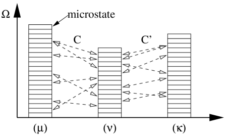
Figure 1: The density of states at different macrostates $\mu$, $\nu$ and $\kappa$ (schematic). For a reversible mechanism the number of connections $C=C(\mu\rightarrow\nu)=C(\nu\rightarrow\mu)$ between two macrostates is the same for the forward and backward transitions.

The consideration underlying our method is relatively simple. Assume at first a classical discrete spin system. A macrostate of the system may for convenience be denoted by $\mu$. One might think of the energy $e_{k}$ and magnetization $m_{l}$ that characterize a macrostate or level $\mu=(e_{k},m_{l})$. In general, a huge number of microstates belongs to a macrostate $\mu$. This number is the degeneracy $Z_{\mu}$ of the level $\mu$. In the course of the simulation a reversible mechanism takes the system from a microstate in a level $\mu$ to a different one which belongs to another level $\nu$. This step is repeated many times. Of course, the same mechanism has to be applied at every update. Starting from one microstate, a number $\mathcal{N}$ of new microstates can be generated. The number $\mathcal{N}$ depends on the mechanism and on the model under consideration.

When the mechanism operates on all microstates of the level $\mu$ then $\mathcal{N}Z_{\mu}$ new microstates can be generated. A number $C(\mu\rightarrow\nu)$ of these belong to the level $\nu$. The quantity of specific interest is $w(\mu\rightarrow\nu)=C(\mu\rightarrow\nu)/\mathcal{N}Z_{\mu}$ which is the probability of arriving at anyone of the microstates belonging to the level $\nu$ when the starting point was one of the microstates of level $\mu$. As the mechanism is reversible the numbers of forward and backward transitions between the levels $\mu$ and $\nu$ are the same: $C(\mu\rightarrow\nu)=C(\nu\rightarrow\mu)$, see Figure 1. This then yields the expression

$$\frac{Z_{\mu}}{Z_{\nu}}=\frac{w(\nu\rightarrow\mu)}{w(\mu\rightarrow\nu)}.$$ (2)

which allows the determination of the degeneracies $Z_{\mu}$ from the transition probabilities $w$. Eq. (2), which is sometimes called Broad Histogram Equation oliv98 , is already complete for discrete spin models like the Ising or Potts models.

Let us now focus on spin models with continuous spin variables. As an example we discuss the $XY$ model muno99 , but the generalization to other models (as for example the Heisenberg model) is straightforward. In our case both the energy and the magnetization have continuous values and the magnetization is a two-dimensional vector. As the energy function (1) is invariant under global spin rotations, it is sufficient for many investigations to consider only the modulus $m$ of the magnetization. This also considerably reduces the amount of resources needed for the numerical simulation of the model. For the purpose of performing this simulation we discretize the energy and the magnetization, the discretized values being denoted by $\hat{e}$ and $\hat{m}$, and call $\delta e$ respectively $\delta m$ the width of the discretization. We thereby allocate all microstates with energies $e$ between $\hat{e}-\delta e/2$ and $\hat{e}+\delta e/2$ and modulus $m$ of the magnetizations between $\hat{m}-\delta m/2$ and $\hat{m}+\delta m/2$ to the same macrostate denoted by $\mu=(\hat{e},\hat{m})$. As the magnetisation ${\bf{m}}=(m_{1},m_{2})$ is a two-dimensional vector the “volume”

$$V(\hat{m})=2\pi\,\hat{m}\,\delta e\,\delta m$$ (3)

in ($e$,$m$)-space is not a constant. The DOS $\Omega(\hat{e},\hat{m})$ is derived from

$$\Omega(\hat{e},\hat{m})=Z(\hat{e},\hat{m})\,/\,V(\hat{m})$$ (4)

where $Z(\hat{e},\hat{m})\equiv Z_{\mu}$. This expression also holds for other models beyond the $XY$ model, where one only has to replace the volume (3) by the appropriate expression. It is important to note that during the simulation the spin variables as well as the energy and the magnetization of the system adopt continuous values. The discretisation only concerns the quantities depending on the macrostates, e. g. the DOS and the transition probabilities.

As already mentioned we perform the simulation with a reversible mechanism. For the $XY$ model we use single spin rotations of randomly selected spins and a random rotation angle $-\pi\leq\varphi<\pi$. The following description of the algorithm is very general and also applies to discrete spin models. Suppose that the system is in a macrostate denoted by $\hat{e}$ and $\hat{m}$ or equivalently by $\mu$. In the next step it is attempted to bring the system into another state $\nu$ by the use of the mechanism described above. We increase the number of attempts $B(\mu)$ to leave the macrostate $\mu$ by one count. At the same time we add one count to $T(\mu\rightarrow\nu)$ which is the number of attempted transitions from $\mu$ to $\nu$. In a long run the ratio $t(\mu\rightarrow\nu):=T(\mu\rightarrow\nu)/B(\mu)$ finally approximates the transition probability $w(\mu\rightarrow\nu)$. It is the quantity $t(\mu\rightarrow\nu)$ which we call transition variable. During the simulation $B(\mu)$ and $T(\mu\rightarrow\nu)$ are updated at every attempted step. The probability of acceptance of the transition from $\mu$ to $\nu$ is chosen to be

$$p:=\min\left[\frac{t(\nu\rightarrow\mu)}{t(\mu\rightarrow\nu)};1\right]$$ (5)

This choice of $p$ leads to an equal number of attempts $B(\mu)$ to leave any macrostate $\mu$, if sufficiently many updates of the system are performed. This is due to the fact, that now the probabilities for an actually executed transition for both the forward and backward directions are equal. It is worth mentioning that the probability of acceptance changes during the simulation and that it approaches its asymptotic value

$$\tilde{p}=\min\left[\frac{w(\nu\rightarrow\mu)}{w(\mu\rightarrow\nu)};1\right]$$ (6)

for very long runs.

II.2 Construction of the entropy surface

Suppose that a macrostate $\mu=(\hat{e},\hat{m})$ whose degeneracy $Z_{\mu}$ has not yet been determined can be reached from several macrostates $\nu$ and suppose that the values of the $Z_{\nu}$ are known, then with the knowledge of the transition probabilities one may calculate $\ln Z_{\mu}$ starting from one of the macrostates with $\nu=\nu^{\prime}$:

$$\ln Z_{\mu}=\ln\frac{w(\nu^{\prime}\rightarrow\mu)}{w(\mu\rightarrow\nu^{\prime})}+\ln Z_{\nu^{\prime}}$$

and one would obtain the same result $\ln Z_{\mu}$ for each of the states $\nu$ as a starting point. However, the simulation only yields the transition variables $t(\mu\rightarrow\nu)$ which are estimates for the transition probabilities $w(\mu\rightarrow\nu)$. Consequently, as these estimates are subject to stochastic fluctuations, we end up with different values for $\ln Z_{\mu}$ when starting from different macrostates $\nu$.

To take this into account we propose to estimate $\ln Z_{\mu}$ by the weighted average

$$\ln Z_{\mu}=\sum\limits_{\nu}p_{\mu\nu}\,\left(\ln\frac{t(\nu\rightarrow\mu)}{t(\mu\rightarrow\nu)}+\ln Z_{\nu}\right)$$ (7)

where the sum is over all macrostates $\nu$ from which the macrostate $\mu$ can be reached. The weights $p_{\mu\nu}$ are given by

$$p_{\mu\nu}=\frac{g_{\mu\nu}}{\sum\limits_{\kappa}g_{\mu\kappa}}$$ (8)

with

$$g_{\mu\nu}=\frac{T(\mu\rightarrow\nu)\,T(\nu\rightarrow\mu)}{T(\mu\rightarrow\nu)+T(\nu\rightarrow\mu)}$$ (9)

which follows from the gaussian error propagation. Another possible choice for the $g_{\mu\nu}$ is given by

$$g_{\mu\nu}=\min\left(T(\mu\rightarrow\nu);T(\nu\rightarrow\mu)\right).$$ (10)

We checked that both choices (9) and (10) lead to microcanonical entropies which, within the errors, are the same.

Up to now we have tacitly assumed that the degeneracies $Z_{\nu}$ entering the sum in Eq. (7) were known exactly. This is of course not the case, the $Z_{\nu}$ being also affected by statistical errors. To reduce the errors in the entropy values we propose the following iterative scheme. At the start we attribute an arbitrary value $\ln Z_{\nu_{0}}=C_{0}$ to a randomly chosen macrostate $\nu_{0}$. Note that the choice of $C_{0}$ does of course not affect our analysis as microcanonically defined physical quantities only involve derivatives of the microcanonical entropy gros01 . Furthermore, if one would use the generated entropy in a canonical analysis, the constant $C_{0}$ would drop out when taking canonical averages of any observable. Having chosen an initial macrostate, we perform a random walk in the parameter space (in our case the energy-magnetization space) and attribute to any visited macrostate $\mu$ the degeneracy $Z_{\mu}$ obtained by evaluating Eq. (7). Of course, in doing so, only macrostates which have in the past been visited at least once can contribute to the sum in Eq. (7). This is repeated until every macrostate has often been visited, typically a few thousand times. When $\ln Z_{\mu}$ has been obtained for all the macrostates $\mu=(\hat{e},\hat{m})$, Eq. (4) yields the microcanonical entropy as (setting $k_{B}=1$)

$$S(\mu)=\ln Z_{\mu}-\ln V(\hat{m}).$$ (11)

It is of advantage not to integrate directly over the whole parameter space, but to restrict the random walk at the beginning to a small area around the starting point $\nu_{0}$, as shown in Figure 2. The area at the start must be large enough to encompass all the macrostates reachable from the macrostate $\nu_{0}$. Typically after a few thousands visits of every macrostate inside the initial area, this integration area is increased. This change of integration area is performed periodically. At some stage we no longer update the center of the integration area, see Figure 2.

The presented method has the advantage that all transition variables computed in the simulation are used for the construction of the entropy. Furthermore, the iterative scheme just described ensures that the error in the final result for the entropy is minimized. It must be noted that this method is of course also applicable for other models, including models with discrete spins, as only the correct volume $V$ has to be inserted into Eq. (11). Finally, we mention that for larger system sizes it is often of advantage to compute the entropy of stripes restricted in energy direction huel02 ; schu03 . The adaption of the presented method to this restricted geometry in the parameter space is straightforward.

 

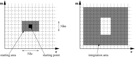
Figure 2: The integration area at the beginning (left figure) and after several extensions (right figure). For this sketch we supposed that the initial point is only reachabel from microstates inside the grey area (left). At later stages, the middle of the integration area is not changed anymore (right).

III Analysis of the entropy

The procedure outlined in the previous Section has been applied to systems of different linear extension $L$ up to $L$ = 25. For most of the runs the size of the channels has been chosen to be unity on the extensive scale, i.e. $\delta e=\delta m=1/N$, though different discretizations have also been tried with no noticeable effect on the results. For $L=10$ this is illustrated in Figure 3 where we show the computed entropy as a function of $m$ for two different fixed values of the energy and two different discretizations. The data obtained for the different discretizations perfectly agree within errors. Note that this is an important point as the independence of the results on the bin size demonstrates that we are indeed accessing continuous properties.

 

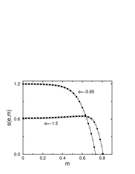
Figure 3: Computed entropy for the three-dimensional $XY$ model with $N=10^{3}$ spins as function of the modulus of the magnetization for two different energies and two different discretizations: $\delta e=\delta m=1/N$ (full symbols) and $\delta e=\delta m=2/N$ (open symbols). The data have been obtained by simulating two different stripes centered at the energies $e=-0.65$ and $e=-1.5$. Only selected points are shown by symbols. Note that for $e=-0.65$ the entropy is maximal for $m=0$, whereas for $e=-1.5$ the maximum is located at $m=m_{sp,L}(e)>0$. For illustrative reasons the data have been shifted vertically by adding a constant.

Whereas for small systems the entropy $s(e,m)$ can be computed in a single run, for larger systems the increasing number of channels in energy and in magnetization direction makes the computation of the entropy very time consuming. One can then restrict the determination of the transition variables to narrow stripes restricted in the energy direction, which permits a distribution of the computation on different CPUs. The width of our stripes was usually 25 units on the extensive energy scale, which corresponds to twice the maximum energy increment in a single move. On the intensive scale the stripes are rather narrow $(\approx 3\cdot 10^{-3})$ for a system with $L=20$. Therefore the resulting entropies can be averaged over the 25 energy channels in order to obtain $s(e,m)$ at the center $e$ of the stripe.

Having the entropy or, equivalently, the density of states at our disposal we can use these data in different ways. Of course, we can compute the canonical partition function from the density of states and then obtain thermal averages of the different quantities of interest as the energy, the susceptibility and so on. Here, we take a different route and directly investigate the microcanonical entropy $s(e,m)$ itself. Recent investigations of discrete spin systems huel02 ; plei04 ; behr05 ; hove04 have shown that critical exponents governing the power law behaviour of quantities in the vicinity of a critical point can be determined reliably by analyzing directly the density of states of finite systems. Here we extend this analysis to phase transitions taking place in classical spin systems with continuous degrees of freedom hove04b . This kind of approach also poses a severe test to our method of computing the entropy, as a microcanonical analysis requires data of extremely high quality due to the absence of the smoothening effect of the Boltzmann weights.

Coming back to our numerical data we observe that the entropy $s(e,m)$, as a function of the modulus of the magnetization, shows one maximum at $m=0$ for $e\geq e_{c,L}$ and one maximum at $m=m_{sp,L}(e)>0$ for $e<e_{c,L}$, see Figure 3. For a given energy $e$ the DOS as function of $m$ exhibits an extremely sharp maximum such that the overwhelming majority of the accessible states belongs to the value of $m$ where $s$ has a maximum. Therefore $m_{sp,L}(e)$ is identified with the spontaneous magnetization of the finite system kast00 ; huel02 ; behr04 ; plei04 . Figure 4 shows the spontaneous magnetization for three system sizes. In order to produce this plot the maximum has been determined for a series of stripes centered at different values of $e$. Notice the sharp onset of $m_{sp,L}(e)$ at $e_{c,L}$, a behaviour also observed for discrete spin models displaying a continuous phase transition in the infinite volume limit kast00 ; huel02 ; plei04 ; behr04 . This onset is accompanied by a divergence of the radial part of the microcanonically defined susceptibility behr04b

$$\chi(e,m)=-\frac{\frac{\partial s}{\partial e}\frac{\partial^{2}s}{\partial e^{2}}}{\frac{\partial^{2}s}{\partial e^{2}}\frac{\partial^{2}s}{\partial m^{2}}-\left(\frac{\partial^{2}s}{\partial e\partial m}\right)^{2}}.$$ (12)

This divergence is due to the fact that the curvature in the radial direction of $m$ (i.e. the denominator in (12)) vanishes at $e_{c,L}$.

 

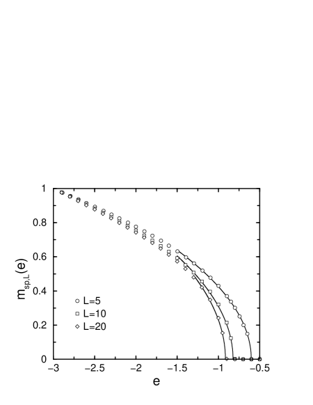
Figure 4: Spontaneous magnetization of the three-dimensional $XY$ model as function of the energy per spin for three different sizes. Note the sharp onset of the spontaneous magnetization at the size-dependent energy $e_{c,L}$. Error bars are much smaller than the sizes of the symbols. Lines are obtained by fitting the data close to $e_{c,L}$ to a square root (13).

Exploiting the fact that close to $e_{c,L}$ the spontaneous magnetization rises with a square root singularity, $e_{c,L}$ can be determined with high precision from a fit of the nonzero values of $m_{sp,L}(e)$ by the expression

$$m_{sp,L}(e)=A_{L}(e_{c,L}-e)^{1/2}$$ (13)

where $A_{L}$ and $e_{c,L}$ are adjustable parameters. The resulting values of $e_{c,L}$ are plotted in Figure 5 as a function of $1/L$ together with the fit function

$$e_{c,L}=e_{c,\infty}+B(1/L)^{\nu_{\epsilon}}$$ (14)

with the adjustable parameters $e_{c,\infty}$, $B$ and $\nu_{\epsilon}$. The fit yields the values $e_{c,\infty}=-0.965(10)$ and $\nu_{\epsilon}=0.666(5)$ which, considering the relatively small systems we have simulated, are in good agreement with the best values found in the literature, namely $e_{c}=-0.9884$ cucc02 and $\nu=0.67155(27)$ camp01 .

 

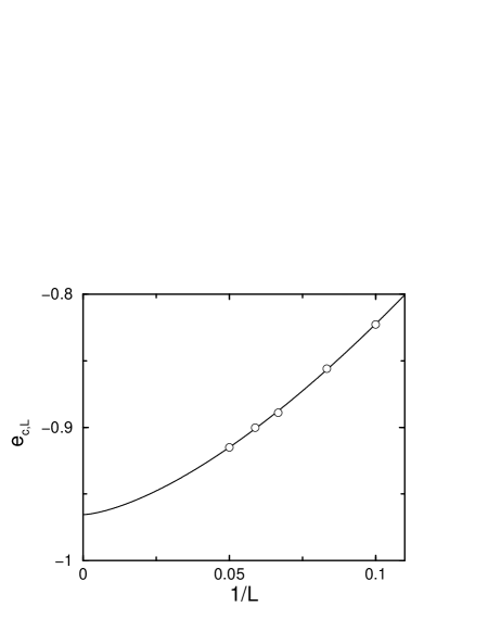
Figure 5: Pseudo-critical energy $e_{c,L}$, defined by the sharp onset of the spontaneous magnetization, as function of the inverse linear extension $1/L$. The full line results from a fit of Eq. (14) to the data points, with $e_{c,\infty}=-0.965$, $B=4.534$ and $\nu_{\epsilon}=0.666$. Error bars are comparable to the symbol size.

We briefly pause to recall that in the entropy formalism considered here critical exponents are not always identical to the better known thermal critical exponents. Indeed, in cases where the specific heat is diverging at the critical point (implying that the thermal critical exponent $\alpha$ governing this divergence is positive, $\alpha>0$) critical exponents $x_{\epsilon}$ appearing in the microcanonical analysis are related to their canonical counterparts $x$ by $x_{\epsilon}=x/(1-\alpha)$ kast00 . This is not so in cases where the specific heat displays a cusp singularity with $\alpha<0$. There $x_{\epsilon}=x$. For the three-dimensional $XY$ model we have $\alpha\approx-0.015$ camp01 and consequently critical exponents obtained in the microcanonical analysis are identical to the thermal critical exponents. We can therefore savely drop the index $\epsilon$ from now on.

For all finite system sizes the expansion (13), which is valid in the vicinity of $e_{c,L}$, yields the classical critical exponent $\beta_{c,L}=1/2$ behr04 , but the range of validity of (13) shrinks to zero with $L\rightarrow\infty$. Outside of this range $m_{sp,L}(e)$ differs very little from $m_{sp}(e)=m_{sp,\infty}(e)$ for not too small system sizes. The critical expansion for the infinite system is given by

$$m_{sp}(e)=A\,\varepsilon^{\beta}$$ (15)

where $\varepsilon=\frac{e_{c}-e}{e_{c}-e_{g}}$ and $e_{g}=-3$ is the ground state energy per degree of freedom. Eq. (15) is stricly speaking only valid in the limit $\varepsilon\longrightarrow 0$. One may analyze the spontaneous magnetization by looking at the energy dependent logarithmic derivative huel02

$$\beta_{eff}(\varepsilon)=\frac{d\ln m_{sp}(\varepsilon)}{d\ln(\varepsilon)}$$ (16)

which approaches the true critical exponent $\beta$ in the limit limit $\varepsilon\rightarrow 0$. Plots which show this approach for the two- and three-dimensional Ising systems can be found in huel02 . Figure 6 shows $\beta_{eff}(\varepsilon)$ of the $XY$ model under study for several lattice sizes. All the graphs, of course, precipitate to zero on approaching $\varepsilon=0$ because $m_{sp,L}(e)$ is finite at $e=e_{c}$, i.e. for $\varepsilon=0$, but the region of constant slope around $\varepsilon=0.5$ can be used to extrapolate the data to $\varepsilon=0$. Figure 7 shows the result of this extrapolation for five values of L. These values quickly come close to the expected value $\beta=0.3485(2)$ camp01 .

 

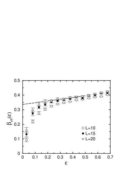
Figure 6: Effective exponents derived from the spontaneous magnetization, see Eq. (16), as function of $\varepsilon$ for different system sizes. The dashed line extrapolates the data for $L=20$ with $0.15<\varepsilon<0.50$ to zero.

 

Figure 7: Variation of $\beta_{\varepsilon,L}$ obtained from extrapolating linearly the effective exponents $\beta_{eff}$ as function of $L$. The dashed line indicates the literature value $\beta=0.3485$ camp01 .

Microcanonical finite-size scaling, as suggested in plei04 , is another way of determining critical exponents. This approach takes advantage of the existence of a well-defined transition point $e_{c,L}$ in finite microcanonical systems and leads to the scaling ansatz

$$L^{\beta/\nu}\,m_{sp,L}\left((e_{c,L}-e)\right)\sim W\left(C\,(e_{c,L}-e)\,L^{1/\nu}\right)$$ (17)

where $W$ is a universal scaling function characterizing the given universality class and $C$ is a nonuniversal constant. It is worth noting that in this approach the knowledge of the value of the critical energy $e_{c}$ of the infinite system is not needed. As shown in plei04 Eq. (17) yields reliable values of the involved critical exponents for discrete models. We show in Fig. 8 that this is also the case for the continuous model discussed here. Plotting L${}^{\beta/\nu}\,m_{sp,L}$ against $(e_{c,L}-e)\,L^{1/\nu}$, we obtain the values $\beta/\nu=0.53(1)$ and $1/\nu=1.47(2)$ from the best data collapse, in good agreement with the expected values camp01 0.5189 and 1.4891.

 

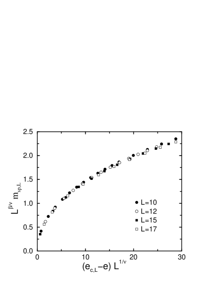
Figure 8: Microcanonical finite-size scaling plot for the three-dimensional $XY$ model. The values $\beta/\nu=0.53(1)$ and $1/\nu=1.47(2)$ result from the best data collapse. Error bars are comparable to the sizes of the symbols.

IV Conclusions

In recent years impressive progress has been achieved in the numerical computation of the DOS of finite classical systems, as new and highly efficient simulation methods have been proposed. One of the aims of this work is the generalization of the method presented in huel02 to systems with continuous degrees of freedom. This method relies on the powerful concept of transition variables oliv98 . In our implementation the actual values of the transition variables are used for the acceptance rates of a proposed move, and this during the entire run. As a consequence all sites of the parameter space are visited with the same rate.

With the final values of the transition variables we can construct the density of states, using the complete information contained in these variables. We have formulated this approach in the present paper for magnetic systems, where the natural variables are given by energy and magnetization, but a generalization to other situations is straightforward.

With the knowledge of the density of states we can analyze the system under investigation in different ways. One common approach is to compute the partition function and then proceed with a canonical analysis. The good quality of our data, however, also enables us to perform a microcanonical analysis where derivatives of the entropy with respect to energy and magnetization play a predominant role. The usefulness of the microcanonical analysis in the study of phase transitions has been revealed in many recent studies gros01 ; huel02 ; plei04 ; gros00 ; huel94 ; behr05 .

The theory of phase transitions is usually formulated within the frame of the canonical ensemble, which is based on the partition function or on its logarithm, the free energy. All the thermodynamic functions, as e.g. the susceptibility, are calculated from derivatives of the free energy with respect to the temperature and the applied fields. For all finite system sizes these derivatives remain finite, but in the thermodynamic limit they may diverge at the critical point, if a continuous phase transition occurs in the system.

In the microcanonical ensemble the analysis of phase transitions is based on the DOS or its logarithm, the entropy gros01 ; behr04 ; gros00 . It has been demonstrated for several discrete spin models that the abrupt onset of the order parameter at $e_{c}$ and the divergence of the susceptibility occurs already for systems consisting of a rather modest number of spins, albeit with the classical values of the critical exponents kast00 ; behr04 .

We have demonstrated in this work that similar features are observed in systems with continuous spins: In a finite system of linear extension $L$ the curvature of the entropy surface in the magnetization direction changes sign at the point $e=e_{c,L}$. It is there where the order parameter sets in and where the susceptibility diverges in continuous as well as in discrete systems. Therefore for the $XY$ model, where $e$ and $m$ take continuous values, the entropy $s(e,m)$ shows the same behaviour as for discrete spin models where it is defined only at discrete points in the parameter space.

Of course, numerical studies must be performed at discrete values of the variables. The distinguishing fact is that for continuous models these values can be chosen freely, such that derivatives can, in principle, be calculated from the ratios of arbitrarily small differences. The reality of a numerical study, however, sets the limits.

As a final application we have demonstrated that in systems with continuous degrees of freedom critical exponents can in principle be determined directly from the density of states, along the same lines as in discrete models huel02 ; plei04 ; behr05 ; hove04 . In particular, we obtain very good estimates of $\nu$ and $\beta$ with regard to the modest system sizes used in this study.

- (1) D. H. E. Gross, Microcanonical Thermodynamics: Phase Transitions in ’Small’ Systems (Lecture Notes in Physic 66) (2001, Singapore: World Scientific).
- (2) M. Kastner, M. Promberger and A. Hüller, J. Stat. Phys. 99, 1251 (2000).
- (3) A. Hüller and M. Pleimling, Int. J. Mod. Phys. C 13, 947 (2002).
- (4) H. Behringer, J. Phys. A: Math. Gen. 37, 1443 (2004).
- (5) M. Pleimling, H. Behringer and A. Hüller, Phys. Lett. A 328, 432 (2004).
- (6) P. M. C. de Oliveira, T. J. P. Penna, and H. J. Herrmann, Eur. Phys. J. B 1, 205 (1998).
- (7) J.-S. Wang, Eur. Phys. J. B 8, 287 (1998).
- (8) J.-S. Wang and L. W. Lee, Comput. Phys. Commun. 127, 131 (2000).
- (9) F. Wang and D. P. Landau, Phys. Rev. Lett. 86, 2050 (2001); Phys. Rev. E 64, 056101 (2001).
- (10) H. Behringer, M. Pleimling, and A. Hüller, J. Phys. A: Math. Gen. 38, 973 (2005).
- (11) F. Sastre, I. Dornic, and H. Chaté, Phys. Rev. Lett. 91, 267205 (2003).
- (12) The reader should note that in muno99b an implementation of the Broad Histogram method to systems with continuous degrees of freedom has been presented. This implementation differs in many aspects from our algorithm. For example, Muñoz and Herrmann did not use the actual values of the transition variables for the acceptance or the rejection of a proposed spin rotation. Furthermore, they did not try to compute the density of states as a function of both the energy and the magnetization.
- (13) J. D. Muñoz and H. J. Herrmann, Int. J. Mod. Phys. C 10, 95 (1999).
- (14) B. J. Schulz, K. Binder, M. Müller, and D. P. Landau, Phys. Rev. E 67, 067102 (2003).
- (15) J. Hove, Phys. Rev. E 70, 056707 (2004).
- (16) In hove04 Hove also considered the density of states of the clock model with (this model yields the model in the limit ) in two dimensions and of the Ginzburg-Landau model in three dimensions. No attempt was made in that work to extract for these models the values of universal critical quantities directly from the density of states.
- (17) H. Behringer, On the structure of the entropy surface of microcanonical systems (Mensch und Buch Verlag, Berlin, 2004).
- (18) A. Cucchieri, J. Engels, S. Holtmann, T. Mendes, and T. Schulze, J. Phys. A 35, 6517 (2002).
- (19) M. Campostrini, M. Hasenbusch, A. Pelissetto, P. Rossi, and E. Vicari, Phys. Rev. B 63, 214503 (2001).
- (20) D. H. E. Gross and E. V. Votyakov, Eur. Phys. J. B 15, 115 (2000).
- (21) A. Hüller, Z. Phys. B 93, 401 (1994).