Bistability and Hysteresis in the Sliding Friction of a Dimer

Abstract

The sliding friction of a dimer moving over a periodic substrate and subjected to an external force is studied in the steady state for arbitrary temperatures within a one-dimensional model. Nonlinear phenomena that emerge include dynamic bistability and hysteresis, and can be related to earlier observations for extended systems such as the Frenkel-Kontorova model. Several observed features can be satisfactorily explained in terms of the resonance of a driven-damped nonlinear oscillator. Increasing temperature tends to lower the resonant peak and wash out the hysteresis.

I Introduction

The friction experienced by atoms, small molecules, and adlayers moving over substrates is an active topic of current research Gnecco . One reason is the desire to understand, at a fundamental level, the origin of friction. The other reason is the wish to acquire expertise in developing nano-devices like nano-motors, nano-wires, and nano-probes. Besides, sliding friction is related to other atomistic processes at surfaces, such as diffusion of atoms and molecules Ala ; Vega ; Braun ; Romero , and motion of long chains Strunz98 ; Strunz98b ; Braun97 ; Paliy ; Braun03 over periodic substrates. That microscopic sliding friction can exhibit nonlinear behavior depending on the sliding regime has been shown in the recent theoretical literature. Strunz and Elmer Strunz98 have studied in detail the nonlinear friction of the Frenkel-Kontorova model and identified the origins of such friction as being the resonance of the sliding velocity with the internal vibration modes of the chain, and the formation of kinks. The latter phenomenon was also studied by Braun et al. Braun97 ; Braun03 . More recently, Fusco and Fasolino Fusco03a ; Fusco03b have identified the same resonance phenomenon in the friction of a smaller object, a dimer moving over a periodic substrate. Gon alves et al. Goncalves04 have analyzed a closely related system in the relaxation regime, i.e. in the absence of external forces, and have given a simple physical explanation of the observed results. Persson Persson93 has predicted that a friction force proportional to $v^{-3}$ is to be expected (in addition to the linear one) in the large-force regime for a sliding system of any size, ranging from a single atom to an infinite chain. In the present paper, we restrict our study to the steady state friction of a dimer, but investigate all force regimes. We identify several separate regimes exhibiting resonance, bistability, and hysteresis. We provide a simple explanation for these phenomena in terms of the resonance of a driven-damped oscillator, and comment on how they depend on the substrate corrugation, damping and temperature.

II Model and Simulation results

At zero temperature, the equations of motion for the two particles constituting the dimer sliding over a periodic potential, in the presence of external force $F$, are Fusco03b ; Goncalves04 :

$$m\ddot{x}_{1}+m\gamma\dot{x}_{1}-k(x_{2}-x_{1}-a)=\frac{2\pi u}{b}\sin\left(\frac{2\pi x_{1}}{b}\right)+F$$

$$m\ddot{x}_{2}+m\gamma\dot{x}_{2}+k(x_{2}-x_{1}-a)=\frac{2\pi u}{b}\sin\left(\frac{2\pi x_{2}}{b}\right)+F,$$ (1)

where $x_{1,2}$ are the coordinates of the two particles each of mass $m$, and $k$, $a$, $b$, $u$ are, respectively, the spring constant, equilibrium length of the dimer, wavelength of the substrate potential and half the amplitude of the potential. We integrate these coupled equations numerically using the algorithm of Verlet modified to allow for velocity-dependent forces Goncalves04 . The underlying characteristic physical quantities in this system are the equilibrium dimer length $a$, the substrate wavelength $b$, the free dimer characteristic time $1/\omega_{0}=\sqrt{m/2k}$, and an energy that describes the dimer oscillation such as $kb^{2}$. In our numerical integrations we use a time step $\Delta t$ equal to $0.03\omega_{0}^{-1}$.

The procedure is as follows: for a fixed value of $F$ we obtain the center of mass velocity $v$, averaged over several thousand time steps in the steady state. Repeating the procedure for several hundreds of different values of the force, we construct a characteristic curve of force versus velocity, $F/(m\gamma)$ versus $v$, (see Fig.1).

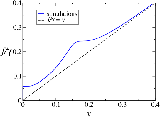
Figure 1: Force–velocity ($f/\gamma$ versus $v$, $f=F/m$) relation obtained from numerical integration in the steady state. Both $f/\gamma$ and $v$ are expressed in units of $b\omega_{0}$. Parameter values are $u=0.038kb^{2},\gamma=(2/3)\omega_{0}$, and $a/b=1/2$. Notice that the maximum friction at resonance occurs when $2\pi v/b\approx\omega_{0}$, therefore for abscissa values which are around $(2\pi)^{-1}$.

The following features are evident from Fig.1 as emerging from our numerical simulations:

1. Existence of a static threshold: there is a minimum value of the externally applied force required to make the dimer slide. It arises from the fact that, at zero temperature, the substrate potential has to be overcome.

2. Linear behavior in the asymptotic large-force regime: for sufficiently large forces, the dimer slides at velocities high enough to make the substrate potential a negligible perturbation. The linear asymptote is shown in Fig.1 as the dashed line.

3. Nonlinearity in the friction exhibiting a maximum: this arises from resonance effects when the washboard frequency $2\pi v/b$ is close in value to the dimer frequency $\omega_{0}=\sqrt{2k/m}$.

The first two of these features are expected in light of previous reports in the literature. The third appears to be interesting. Previous related reports have been on the driven diffusion of a dimer Fusco03b , and of a Frenkel-Kontorova model in the presence of an external force Strunz98 . A thorough analysis is however lacking. We attempt to provide such an analysis below in the specific case of the dimer. We relate our results to observations made by other authors in the context of the Frenkel-Kontorova model, and suggest that the essential features of the nonlinear friction of the infinite linear chain can be understood in terms of the dimer dynamics we describe.

III Simple theoretical considerations

A transformation of the coordinates of the two dimer masses to the center of mass coordinate $x_{+}=(x_{2}+x_{1})/2$, and the internal coordinate $x_{-}=(x_{2}-x_{1})/2$, converts Eqs.(1) to

$$\ddot{x}_{+}+\gamma\dot{x}_{+}= \frac{2\pi u}{mb}\sin\left(\frac{2\pi x_{+}}{b}\right)\cos\left(\frac{2\pi x_{-}}{b}\right)+F/m$$

$$\ddot{x}_{-}+\gamma\dot{x}_{-}+\frac{k}{m}(2x_{-}-a)= \frac{2\pi u}{mb}\sin\left(\frac{2\pi x_{-}}{b}\right)\cos\left(\frac{2\pi x_{+}}{b}\right).$$ (2)

If in the last equation we define $\xi=\frac{2x_{-}}{a}-1=\frac{x_{2}-x_{1}}{a}-1$, we get

$$\frac{d^{2}\xi}{dt^{2}}+\gamma\frac{d\xi}{dt}+\omega_{0}^{2}\xi=\frac{4\pi u}{mba}\sin\left(\frac{\pi a}{b}(1+\xi)\right)\cos\left(\frac{2\pi x_{+}}{b}\right)$$ (3)

as in the analysis of Ref. Goncalves04 . Contrary to that analysis, however, here our interest lies in the steady state reached after the application of the external force. In that state, the center-of-mass velocity $v_{+}(t)$ oscillates around a constant value $v$. Considering only situations in which $\Delta v(t)=|v_{+}(t)-v|<v$, let us neglect $\Delta v(t)$ and decouple the equations. The internal coordinate then satisfies

$$\frac{d^{2}\xi}{dt^{2}}+\gamma\frac{d\xi}{dt}+\omega_{0}^{2}\xi=\frac{4\pi u}{mba}\sin\left(\frac{\pi a}{b}(1+\xi)\right)\cos(\omega t),$$ (4)

which describes a damped nonlinearly driven oscillator. The natural frequency is $\omega_{0}=\sqrt{2k/m}$, the damping is $\gamma$, and the driving frequency $\omega$ is proportional to the constant component of the center of mass velocity: $\omega=2\pi v/b$ which is the so-called washboard frequency.

III.1 Linear analysis in zeroth order

Eq.(4) cannot be solved analytically because of the nonlinearity in the sine term. The simplest approximation, valid in zeroth order in powers of $\xi$, leads to the equation of a driven-damped linear oscillator:

$$\frac{d^{2}\xi}{dt^{2}}+\gamma\frac{d\xi}{dt}+\omega_{0}^{2}\xi=\frac{4\pi u}{mba}\sin\left(\frac{\pi a}{b}\right)\cos(\omega t),$$ (5)

with an exact solution in the steady state,

$$\xi(t)=\frac{4\pi u}{mba}\sin\left(\frac{\pi a}{b}\right)\frac{1}{\sqrt{\left(\omega_{0}^{2}-\omega^{2}\right)^{2}+\omega^{2}\gamma^{2}}}\cos\left(\omega t-\delta\right),$$ (6)

where $\delta$ is the phase angle given by $\tan(\delta)=\frac{\gamma\omega}{\omega_{0}^{2}-\omega^{2}}$. In order to compute the dependence of the friction on the center-of-mass velocity, we must resort to the power balance condition which, in terms of the averaged center-of-mass and internal velocity, can be written as

$$F<v_{+}>=m\gamma<v_{+}^{2}>+m\gamma<v_{-}^{2}>.$$ (7)

Defining $f=F/m$, and using the previously made assumption that $<v_{+}^{2}>\approx v^{2}$, leads to

$$f=\gamma v+\gamma\frac{<v_{-}^{2}>}{v}.$$ (8)

We see that, generally, the steady-state friction the center of mass of the dimer experiences is nonlinear in the velocity. Using the steady state solution for $\xi(t)$ as given by (6), we calculate

$$<v_{-}^{2}>=\frac{1}{2}\left(\frac{2\pi u}{mb}\right)^{2}\sin^{2}\left(\frac{\pi a}{b}\right)\frac{\omega^{2}}{\left(\omega_{0}^{2}-\omega^{2}\right)^{2}+\omega^{2}\gamma^{2}}.$$ (9)

Substitution of $<v_{-}^{2}>$ given by Eq.(9) in Eq.(8), yields

$$\frac{f}{\gamma}-v=\frac{1}{2}\left(\frac{u}{m}\right)^{2}\sin^{2}\left(\frac{\pi a}{b}\right)\frac{v}{\left(v^{2}-(b\omega_{0}/2\pi)^{2}\right)^{2}+v^{2}(b\gamma/2\pi)^{2}}.$$ (10)

The right hand side of Eq.(10) focuses on the nonlinear component of the friction. In Fig.2 we plot Eq.(10) together with the exact results from the simulations. We see that our zeroth order theory captures the essence of the resonance behavior, approximates well the location of the peak, is excellent quantitatively for larger velocities, and fails only to describe the low-velocity threshold.

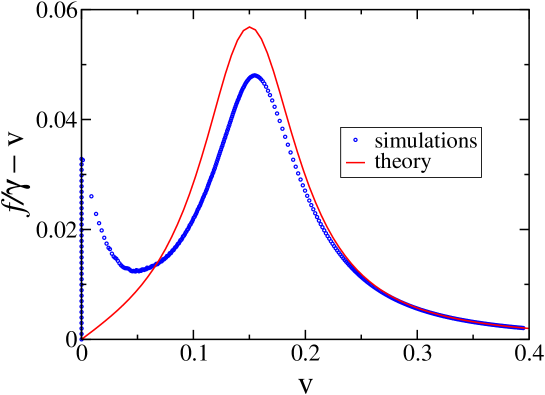
Figure 2: Resonance effect in the nonlinear friction of the dimer and comparison of the simulations with the zeroth order theory. Plotted is the nonlinear part, $f/\gamma-v$ of the characteristic curve for a dimer sliding over a periodic substrate. Circles are from numerical integration at the steady state. The solid line is the zeroth order theory for the uncoupled equation for $\xi$. $f/\gamma$ and $v$ are both in units of $b\omega_{0}$. The parameters in this case are $u=0.028kb^{2},\gamma=(2/3)\omega_{0}$, and $a/b=1/2$.

In the limit of high velocities ($v>>b\omega_{0}/2\pi,b\gamma/2\pi$), the leading term in the resonance denominator is quartic in $v$, resulting in the following nonlinear friction:

$$\frac{f}{\gamma}-v=\frac{1}{2}\left(\frac{u}{m}\right)^{2}\sin^{2}\left(\frac{\pi a}{b}\right)\frac{1}{v^{3}}.$$ (11)

This agrees with the $1/v^{3}$ result of the sliding friction of the purely internally damped dimer studied recently Goncalves04 . In the other limit, in the low-velocity regime ($v<<b\omega_{0}/2\pi$), the denominator of the right hand side of Eq.(10) is independent of $v$ (it is of fourth order in $\omega_{0}$), so $f/\gamma-v$ in this case becomes linear:

$$\frac{f}{\gamma}-v=\frac{1}{2}\left(\frac{u}{mv_{s}^{2}}\right)^{2}\sin^{2}\left(\frac{\pi a}{b}\right)v.$$ (12)

Here $v_{s}=b\omega_{0}/2\pi$ is the sliding velocity near resonance. Thus, in the limit of typical velocities of experiments, like the microbalance experiment, we recover the linear regime in which $\frac{1}{2}\gamma\left(\frac{u}{mv_{s}^{2}}\right)^{2}\sin^{2}\left(\frac{\pi a}{b}\right)$ represents the part of the friction directly contributed by the interaction with the substrate potential. However, the threshold effect in the dimer problem at $T=0$ prevents this regime from being observed. For an extended object and/or at $T>0$, where the threshold could be vanishing, it would be possible in principle to observe this regime.

III.2 Parametric oscillator in the first order

The zeroth order description fails when $a/b$ is commensurate, i.e. when takes integer $n$ values. In this case the zeroth order approximation cannot be applied and one is forced to go to the next order, since neglecting $\xi$ in the sine terms predicts an erroneous (vanishing) nonlinear friction. In such cases, and if $\xi<<1$,

$$\sin\left(\frac{\pi a}{b}(1+\xi)\right)=(-1)^{n}\sin(n\pi\xi)\approx(-1)^{n}n\pi\xi.$$ (13)

Substitution converts the driven-damped harmonic oscillator equation (4) into the equation for a parametric oscillator

$$\frac{d^{2}\xi}{dt^{2}}+\gamma\frac{d\xi}{dt}+\left(\omega_{0}^{2}+(-1)^{n+1}\frac{4n\pi^{2}u}{mba}\cos(\omega t)\right)\xi=0.$$ (14)

For this equation an exponential increase of $\xi$ is expected in an instability window around $\omega=2\omega_{0}$. Thus, in this regime, $<v_{-}^{2}>$ would increase indefinitely and the friction force would be infinite, which is of course unphysical. In fact, in the full system Eq.(2), the coupling between the center-of-mass and internal motion drives the center of mass out of the instability window characterizing the parametric oscillator, and this is enough to make the increase of $\xi$ saturate Fusco03a ; Fusco03b , yielding a finite value of $<v_{-}^{2}>$. Besides, if $\xi$ increased because of the resonance, the assumption (13) that leads to the parametric oscillator equation (14) would not be valid.

The zeroth order approach predicts that the shape of the resonance is proportional to $\sin^{2}(\pi a/b)$. Accordingly, there are two extreme cases worth discussing: $a/b=0.5+n\pi$ in which the resonance is maximum, because the counter phase movement of the particles makes this the most energy effective case; in contrast $a/b=n\pi$ is the less effective one, since the in phase movement does not excite the internal vibration, thus yielding purely linear friction. The latter case is precisely the one discussed in this section. Figure 3 illustrates the previous discussion showing how the resonance is actually affected by the commensuration ratio $a/b$. Those are results of the numerical integration of Eqs.(1), where we can see that the zeroth order approximation is very good indeed. In the case $a/b=1$, although the friction is not exactly the linear one, there is no resonance at all and the $f$–$v$ characteristic is very close to the linear one. In the inset however, we can see that there is nonlinear friction which goes asymptotically $v^{-3}$ to the linear regime, due to the parametric resonance.

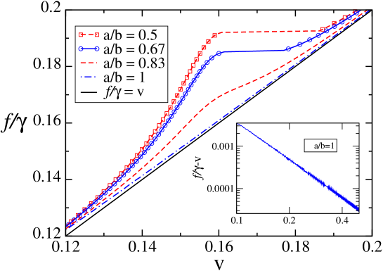
Figure 3: Force–velocity relation obtained from numerical simulation for different values of $a/b$. Notice how the resonance is attenuated as $a/b$ takes on increasing values from 0.5 to 1 and how the case $a=b$ is very close to the linear regime. The difference can only be appreciated in the inset where $f/\gamma-v$ versus $v$ is plotted on log-log scale. $f/\gamma$ and $v$ are both in units of $b\omega_{0}$. Parameter values are $u=0.0056kb^{2},\gamma=(1/6)\omega_{0}$.

III.3 A non-standard description in higher order

A non-standard approximation procedure may be developed through an iterative procedure by noticing that, as the value of an arbitrary variable $y$ increases, the expression $\cos(\kappa\cos(y))$, where $\kappa$ is a constant, oscillates around the value $J_{0}(\kappa)$, whereas $\sin(\kappa\cos(y))$ oscillates around $0$, $J_{0}$ being the Bessel function of order $0$. We have seen that, considered in zeroth order, Eq.(4) predicts that $\xi(t)$ oscillates sinusoidally with frequency $\omega$ (see (6)). Writing $p=\pi a/b$, we may use the fact that

$$<\sin\left(p(1+\xi(t))\right)>\approx<\sin(p)\cos(p\xi(t))>=\sin(p)J_{0}\left(pA\sin(p)Z(\omega)\right),$$ (15)

where $A=\frac{4\pi u}{mba}$ and $Z(\omega)=\frac{1}{\sqrt{\left(\omega_{0}^{2}-\omega^{2}\right)^{2}+\omega^{2}\gamma^{2}}}$. This procedure can be followed iteratively to whatever degree is desired. The successive approximations to the steady state $\xi(t)$ are thus

$$\xi^{0}(t) = A\sin(p)Z(\omega)\cos(\omega t-\delta)$$

$$\xi^{1}(t) = A\sin(p)Z(\omega)J_{0}\left(pA\sin(p)Z(\omega)\right)\cos(\omega t-\delta)$$

$$\xi^{2}(t) = A\sin(p)Z(\omega)J_{0}\left(pA\sin(p)Z(\omega)J_{0}\left(pA\sin(p)Z(\omega)\right)\right)\cos(\omega t-\delta)...$$ (16)

Generally, this may be expressed by defining $\eta=A\sin(p)Z(\omega)$ and writing the approximation as

$$\xi(t)\approx\eta J_{0}(p\eta J_{0}(p\eta J_{0}(p\eta J_{0}(p\eta...))))\cos(\omega t-\delta).$$ (17)

The spectrum predicted through this approximation is seen to be proportional to $\omega^{2}\eta^{2}J_{0}^{2}(p\eta J_{0}(p\eta J_{0}(p\eta J_{0}(p\eta...))))$ to whatever degree of approximation one requires, except for $p\approx n\pi$, in which case the approximation is not valid, for the same reason explained in the previous section.

The left panel of Fig.4 shows a comparison of different orders of this non-standard approximation with the numerical solution of Eq.(4), shown as a solid line. The zeroth order approximation in this procedure, shown as dotted line, overestimates the height of the resonance peak, while the first order approximation, shown as dashed-dotted line, underestimates it. In the second order, shown as dashed line, our procedure is already able to essentially coincide completely with the numerical solution. It is important to realize that our non-standard procedure does very well within the second order when viewed as an approximation to Eq.(4), for which it has been developed, rather than to the original Eqs.(1). The right panel shows the comparison of the numerical solution of Eq.(4), in which the center of mass velocity is a constant, with the simulation based on the original Eqs.(1). One can see a low-velocity departure arising from the static threshold and a high-velocity departure arising from bistability. Such differences arise from the fact that in Eqs.(1) the center-of-mass velocity is itself decided by the dynamics, therefore not being a free parameter as in Eq.(4).

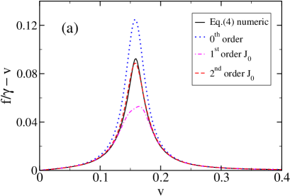
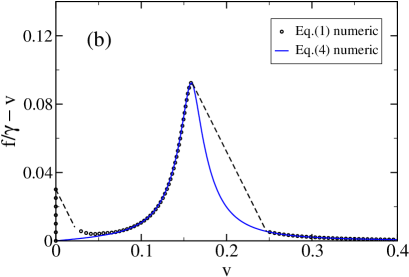
Figure 4: Validity of a non-standard approximation procedure. Plotted is: $f/\gamma-v$ versus $v$, both in units of $b\omega_{0}$. (a) Comparison between the numerical simulation of Eq.(4) for the internal coordinate $\xi$, with the nonstandard approximation in various orders, showing excellent convergence within the $2^{nd}$ order. (b) Comparison between exact solution of system (1) with the solution of Eq.(4), in which the center of mass velocity is a free parameter; notice that except for the discontinuities the agreement is excellent. Parameter values are $u=0.016kb^{2},\gamma=(1/4)\omega_{0}$, and $a/b=1/2$.

IV Further Nonlinear Results

IV.1 Bistability and Hysteresis

The nonlinearities present in our system give rise to bistability. This can be seen in Fig.5 where it is clear that one value of the force can correspond to two distinct values of the velocity, in a certain region. In order to gain deeper insight into this issue, we plot in Fig.5(b) the prediction for the characteristic curve based on expression (10) as $u$ increases. We see features typical of bistable systems such as encountered in the pressure-volume ($p$–$V$) diagram of a van der Waals gas.

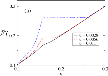
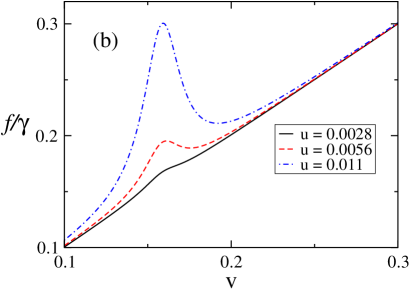
Figure 5: Force–velocity curves $f/\gamma$ versus $v$ (both in units of $b\omega_{0}$) for different values of the corrugation amplitude $u$ expressed in units of $kb^{2}$. Parameter values are: $a/b=0.5,\gamma=(1/6)\omega_{0}$. (a) Simulation results (numerical integration of Eqs.(1)). (b) Zeroth order approximation (Eq.(10)). Notice in both panels that the critical value of $u$ (i.e. the value at which the bistability develops) is around $0.004kb^{2}$ for the chosen values of parameters.

The bistability of the dimer is directly related to hysteresis. Fig.6 shows the presence of two regions, identified by the dashed lines, where hysteresis occurs when the force is first increased from $f=0$ and then is decreased in small steps down to $f=0$. The first hysteresis at low velocities is due to the bistability between the locked and the running state and has a static origin, being associated with the energy threshold that the particle has to overcome in order to move. The same kind of hysteresis is also found in the underdamped monomer Risken . On the other hand, the second hysteresis at intermediate values of $v$ is of purely dynamical nature, and it is related to the bistability between two running states in that region. Let us discuss the latter hysteresis in more detail. Five regions, denoted by roman numbers, can be identified there : I) the mechanically stable region where $v$ increases with $F$ up to a point where the force begins to be bivaluated, II) the metastable region where $v$ increases with $F$ up to the local maximum, III) the mechanically unstable region where $v$ decreases with $F$ up to the local minimum, IV) the metastable region, where $v$ increases with $F$ from the local minimum up to a point where the force ends to be bivaluated, and V) the mechanically stable region where $v$ increases again with $F$ and it is monovaluated. Region I) and V) are both obtained either increasing the force from zero or decreasing it from a high value. Region II, however is accessible while increasing the force from zero but not when the force is decreased from a high value. Complementary, region IV is obtained while decreasing the force from a high value but not when the force is increased from zero. Region III) is mechanically unstable, i.e the velocity decreases when the external force is increased. For a given value of the external force, the system goes to a stable point, therefore when the force goes beyond the value at the local maximum there is a jump from region II to region V. Conversely when the force is decreased from region V the system enters the metastable region IV until at the local minimum it jumps to region I. Notice that, except for the unstable region III, all the hysteresis features of the system are excellently reproduced by the solution of Eq.(4).

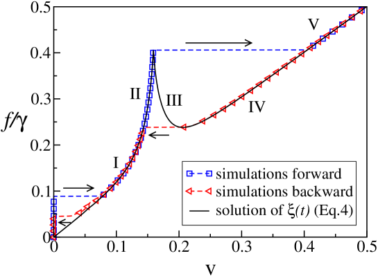
Figure 6: Hysteresis in the force–velocity relation. Symbols are results from simulations of the system Eqs.(1): ($\square$) increasing the external force, ($\lhd$) decreasing the external force. The solid line is the result of numerical integration of the Eq.(4). I and V indicate the stable regions (overlap of the two symbols), II and IV are metastable regions, while III denotes the unstable region. The arrows indicate the forward jumps ($\rightarrow$) and backward jumps ($\leftarrow$). Plotted is $f/\gamma$ versus $v$ (expressed in units of $b\omega_{0}$). Parameter values are $u=0.023kb^{2},\gamma=(1/6)\omega_{0}$, and $a/b=1/2$.

Fig.7 shows the behavior of the center-of-mass velocity for two different, but close, values of the external force near the region of bistability. In the early stages of the dynamics the velocity is practically the same in the two cases, but after some time the velocity corresponding to the lower force attains a steady state value that is much smaller than the one corresponding to the larger force. This clearly illustrates the dynamical origin of the bistability. Furthermore, the oscillations of $v_{+}$ in the steady state are much smaller for the larger force. The bistable behavior of the dimer critically depends on the parameters $u$, $\omega_{0}$ and $\gamma$: For fixed $\omega_{0}$ and $\gamma$, it is observed when $u$ exceeds a critical value, which can be estimated in the framework of the zeroth order approximation as the value for which the local maximum and the local minimum in the velocity-force characteristic, given by Eq.(10) by adding the linear term in $v$, coincide. This is related, in the van der Waals analogy, to the region of coexisting phases. The interplay between linear and nonlinear friction due to resonance gives rise to the bistability, as does the interplay between attractive and repulsive terms in the van der Waals gas. In this sense, Eq.(10) might be regarded as an equation of state of the system. Both equations are however only approximate descriptions of the real system and cannot predict what happens in the transition region, where a coexistence of two different states is found.

Since the hysteresis is intimately linked to the bistability, it appears only for large $u$ (and/or small $\gamma$), as discussed above.

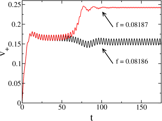
Figure 7: Bistable behavior exhibited in the time evolution of the center-of-mass velocity for slightly different values of the external force $f=F/m$. Velocity $v_{+}$ is in units of $b\omega_{0}$, time $t$ in units of $\omega_{0}^{-1}$, and $f$ in units of $kb$. Notice that, up to time $t=60\omega_{0}^{-1}$, the two curves follow almost the same dynamics, but then separate, respectively, to a low and high limit. Parameters are $u=0.011kb^{2},\gamma=(1/6)\omega_{0}$, and $a/b=1/2$.

IV.2 Effects of non-zero temperature

It is natural to inquire into the effects of finite temperature in our system. We solve Eqs.(1) by adding random forces representing the thermal interaction with the substrate, in the Langevin approach:

$$m\ddot{x}_{1}+m\gamma\dot{x}_{1}+k(x_{2}-x_{1}-a)=\frac{2\pi u}{b}\sin\left(\frac{2\pi x_{1}}{b}\right)+R_{1}+F$$

$$m\ddot{x}_{2}+m\gamma\dot{x}_{2}-k(x_{2}-x_{1}-a)=\frac{2\pi u}{b}\sin\left(\frac{2\pi x_{2}}{b}\right)+R_{2}+F,$$ (18)

in which the stochastic forces $R_{1,2}$ satisfy the conditions

$$<R(t)> = 0$$

$$<R(t)R(t^{\prime})> = 2\gamma mk_{B}T\delta(t-t^{\prime}),$$ (19)

where $k_{B}$ is Boltzmann’s constant and $T$ is temperature. Fig.8 illustrates the velocity-force characteristics at finite temperature, for different values of $T$. By increasing $T$, the effects we have shown at $T=0$ are increasingly smeared out. In particular, the static threshold disappears, as can be seen in the inset of the left panel of Fig.8. The bistability regions and hysteresis still survive up to small values of $T$, and the characteristic curve is smoothened in the region of dynamical bistability. Interestingly, the area of the hysteresis loop, shown in the right panel of Fig.8, decreases with $T$ and eventually disappears for sufficiently high temperatures. A hysteretic behavior in the intermediate friction region, at $T\neq 0$, has been reported for long periodic chains Braun97 . Here we see that we recover essentially the same behavior in the case of the dimer. This is because the same mechanisms are effective, as will be discussed in the next section.

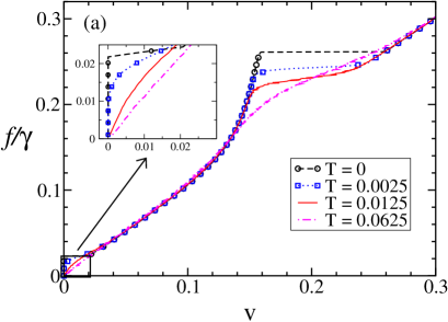
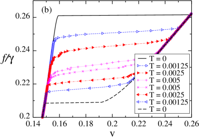
Figure 8: Temperature effects on the force–velocity relation. Plotted is the $f/\gamma$ versus $v$ relation as temperature $T$ (expressed in units of $u/k_{B}$) is varied. $f/\gamma$ and $v$ are in units of $b\omega_{0}$, and parameters are $u=0.011kb^{2},\gamma=(1/6)\omega_{0}$, and $a/b=1/2$. (a) Curves for increasing force, the inset shows the details in the static threshold region. The bistability is seen to disappear as $T$ increases smoothening the characteristic $f$–$v$ curve. (b) Forward and backward curves to emphasize the hysteresis dependence on temperature: the area of the hysteresis loop decreases with $T$ and disappears for temperatures close to $k_{B}T=0.005u$.

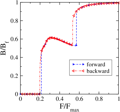
Figure 9: Mobility $B=<v>/F$, normalized by the asymptotic mobility at large forces $B_{f}=(m\gamma)^{-1}$, as a function of the driven force $F$. This plot should be compared to that given for the Frenkel-Kontorova model by Braun et al. Braun97 (see their Fig.1a). The force is normalized by the maximum applied value $F_{max}=0.71kb$. The parameters in this case are $u=0.056kb^{2},\gamma=(2/3)\omega_{0}$, and $a/b=1/2$.

V concluding remarks

Our general aim in the present paper has been to extend previous investigations Goncalves04 of friction in the simplest non-trivial system, a dimer moving over a periodic substrate, to include a driving force and arbitrary temperatures. Our study has shed some light on puzzling features in the literature for more complex systems, such as the Frenkel-Kontorova chain, by allowing us to obtain simple physical arguments for our system. The model is indeed simple: a linear damped oscillator sliding in a sinusoidal periodic potential. Yet, except for the limitation that it is restricted to a single spatial dimension, it has the necessary ingredients to represent a real dimer or molecule set in a controlled microscopic sliding experiment. For example, a molecule sliding along channels of a crystalline well-oriented substrate Kurpick should exhibit some of the features we have described. Our results, both analytical and numerical, confirm the existence of nonlinear friction, resonance effects, bistability, and hysteresis, which can be well understood in terms of the resonance of a driven, damped oscillator. Far from resonance the sliding friction goes asymptotically to the linear regime with a $v^{-3}$ term, which represents the tail of the resonance response. For intermediate forces, bistability and hysteresis emerge as a consequence of the interplay between linear friction and resonance. That our results provide a simple representation of phenomena reported for large systems should be clear from Fig.9, which shows a comparison between our results on the dimer and results from Braun et al. Braun97 for the Frenkel-Kontorova model, which can be regarded as the infinite-size generalization of the dimer. Those results are presented to facilitate direct comparison with Fig.1a of Ref Braun97 in terms of the mobility $B=v/F$, normalized by its asymptotic value $B_{f}=1/m\gamma$. We notice that the intermediate behavior before the asymptotic linear regime is observed in the same fashion as for the dimer. In the latter case the mechanism is completely understood as being due to resonance of the dimer; the same mechanism could also underlie the nonlinear friction in the Frenkel-Kontorova case (see Ref. Strunz98 ). Braun at al. Braun97 attributed such features to the presence of kinks that can be observed during the sliding regime of the Frenkel-Kontorova chain.

In light of the present study, let us make some comments that might have some relevance to the ongoing debate in the literature Smith ; Persson96 ; Tomassone97 ; Liebsch99 about whether sliding friction is mainly electronic or phononic in origin. For this purpose let us identify the background (linear) friction in our model with electronic and the resonance friction with phononic sources. Such an identification appears natural because, although vibrations of the substrate do not exist in our model, resonance friction does arise from the interaction of the dimer vibrations with the substrate; on the other hand, the source of the intrinsic friction, denoted in our analysis by $\gamma v$, is independent of interactions with the substrate. We have seen from our analysis that the resonance friction is modulated by $sin^{2}(\pi a/b)$. The commensuration ratio $a/b$ appearing in this modulation factor would depend in a realistic 2-d or 3-d environment additionally on the relative orientation of the dimer (adlayer) and the substrate. Therefore, while resonance friction might dominate the background friction in principle (for sufficiently large corrugation amplitude values $u$), the smallness of the modulation ratio could make it have disparately small values relative to background friction. That might be a plausible explanation for the disparate results obtained in otherwise similar simulation models Smith ; Persson96 ; Tomassone97 ; Liebsch99 . However, rather high velocities seem to be necessary for resonance friction to be appreciable. Rough estimates we have made suggest that in a number of materials, $b\approx 2$Å, $\omega_{0}\approx 10-100$ cm^-1, adlayer velocities relative to the substrate necessary for resonance friction to be observable would be as high as $30-300$ m/s. The velocity region of the quartz microbalance experiments corresponds to the low velocity limit discussed at the end of section III.1 (see Eq.12) where the resonance friction becomes linear and the ratio between phononic and electronic friction results proportional to $\left(\frac{u}{k^{2}b^{2}}\right)^{2}$. Let us extend this estimation to the case of a Lennard-Jones model for the dimer (adsorbate) interaction, where that ratio becomes proportional to $(u/\epsilon)^{2}$, $\epsilon$ being the well depth of the Lennard-Jones potential. In the Xe over Ag case for example $\epsilon\approx 20$meV and $u$ can lie in the 1-2meV range, therefore the prefactor $(u/\epsilon)^{2}\approx 0.01$. With the above suggested identification of the friction mechanisms —and within the validity of analytical assumption used in the low velocity limit—, one might thus expect phononic friction to be rarely observable for most materials under typical experimental conditions.

VI acknowledgments

This work was supported in part by a grant made by the Los Alamos National Laboratory to the Consortium of the Americas of the University of New Mexico, and by the National Science Foundation under grants INT-0336343 and DMR-0097204. S.G. and C.F. acknowledge the hospitality of the Department of Physics and Astronomy of the University of New Mexico, during their stay at the Consortium of the Americas. Work at Los Alamos is supported by the USDOE.

VII references

References

- (1) E. Gnecco, R. Bennewitz, T. Gyalog and E. Meyer, J. Phys.: Cond. Matt. 13, R619 (2001).
- (2) B. Ala-Nissila, R. Ferrando and S. C. Ying, Adv. Phys. 2002, 51, 949.
- (3) J. L. Vega, R. Guantes and S. Miret-Artés, J. Phys. Condens. Matter 14, 6193 (2002).
- (4) O. M. Braun, R. Ferrando and G. E. Tommei, Phys. Rev. E 68, 051101 (2003).
- (5) A. H. Romero, A. M. Lacasta and J. M. Sancho, Phys. Rev. E 69, 051105 (2004).
- (6) T. Strunz and F.-J. Elmer, Phys. Rev. E 58, 1601 (1998).
- (7) T. Strunz and F.-J. Elmer, Phys. Rev. E 58, 1612 (1998).
- (8) O. M. Braun, T. Dauxois, M.V. Paliy and Michel Peyrard, Phys. Rev. E 55, 3598 (1997).
- (9) M. Paliy, O. Braun, T. Dauxois and B. Hu, Phys. Rev. E 56, 4025 (1997).
- (10) O. M. Braun, Hong Zhang, Bambi Hu, and J. Tekic Phys. Rev. E 67, 066602 (2003).
- (11) C. Fusco and A. Fasolino, Eur. Phys. J. B 31, 95 (2003).
- (12) C. Fusco and A. Fasolino, Thin Solid Films 428, 34 (2003).
- (13) S. Gon alves, V. M. Kenkre and A. R. Bishop, Phys. Rev. B 70, 195415 (2004).
- (14) B. N. J. Persson, Phys. Rev. B 48, 18140 (1993).
- (15) H. Risken, The Fokker-Planck Equation, 2nd ed., Springer (1989).
- (16) U. Kürpick, Phys. Rev. B 63, 045409 (2001); P. J. Feibelman, Phys. Rev. B 61, R2452 (2000); F. Montalenti and R. Ferrando. Surf. Sci. 432, 27 (1999).
- (17) B. N. J. Persson, Sliding Friction, 2nd edn., Springer-Verlag, Berlin, Heidelberg 2000 (and references therein).
- (18) E. D. Smith, M. O. Robbins and M. Cieplak, Phys. Rev. B 54, 8252 (1996).
- (19) B. N. J. Persson and A. Nitzan, Surf. Sci. 367, 261 (1996).
- (20) M. S. Tomassone, J. B. Sokoloff, A. Widom, and J. Krim, Phys. Rev. Lett. 79, 4798 (1997).
- (21) A. Liebsch, S. Gon alves and M. Kiwi, Phys. Rev. B 60, 5034 (1999).