Random close packing revisited: How many ways can we pack frictionless disks?

Abstract

We create collectively jammed (CJ) packings of $50$-$50$ bidisperse mixtures of smooth disks in 2d using an algorithm in which we successively compress or expand soft particles and minimize the total energy at each step until the particles are just at contact. We focus on small systems in 2d and thus are able to find nearly all of the collectively jammed states at each system size. We decompose the probability $P(\phi)$ for obtaining a collectively jammed state at a particular packing fraction $\phi$ into two composite functions: 1) the density of CJ packing fractions $\rho(\phi)$, which only depends on geometry and 2) the frequency distribution $\beta(\phi)$, which depends on the particular algorithm used to create them. We find that the function $\rho(\phi)$ is sharply peaked and that $\beta(\phi)$ depends exponentially on $\phi$. We predict that in the infinite system-size limit the behavior of $P(\phi)$ in these systems is controlled by the density of CJ packing fractions—not the frequency distribution. These results suggest that the location of the peak in $P(\phi)$ when $N\rightarrow\infty$ can be used as a protocol-independent definition of random close packing.

I Introduction

Developing a statistical mechanical description of dense granular materials, structural and colloidal glasses, and other jammed systems book composed of discrete macroscopic grains is a difficult, long-standing problem. These amorphous systems possess an enormously large number of possible jammed configurations; however, it is not known with what probabilities these configurations occur since these systems are not in thermal equilibrium. The possible jammed configurations do not occur with equal probability—in fact, some are extremely rare and others are highly probable. Moreover, the likelihood that a given jammed configuration occurs depends on the protocol that was used to generate it.

Despite difficult theoretical challenges, there have been a number of experimental and computational studies that have investigated jammed configurations in a variety of systems. The experiments include studies of static packings of ball bearings bernal ; scott , slowly shaken granular materials knight ; phillippe , sedimenting colloidal suspensions kegel , and compressed colloidal glasses zhu . The numerical studies include early Monte Carlo simulations of dense liquids finney , collision dynamics of growing hard spheres lubachevsky , serial deposition of granular materials under gravity pavlovitch ; tkachenko ; barker , various geometrical algorithms jodrey ; clarke ; speedy , compression and expansion of soft particles followed by energy minimization ohern_long , and other relaxation methods zinchenko .

Figure 1: The probability distribution $P(\phi)$ to obtain a collectively jammed state at packing fraction $\phi$ in 2d bidisperse systems with $N=18$ (dotted), $32$ (dashed), $64$ (dot-dashed), and $256$ (solid).

The early experimental and computational studies found that dense amorphous packings of smooth, hard particles frequently possess packing fractions near random close packing $\phi_{\rm rcp}$, which is approximately $0.64$ in $3d$ monodisperse systems berryman and $0.84$ in the $2d$ bidisperse systems discussed in this work speedy ; ohern_short . However, more recent studies have emphasized that the packing fraction attained in jammed systems can depend on the process used to create them. Different protocols select particular configurations from a distribution of jammed states with varying degrees of positional and orientational order torquato_2000 .

Recent studies of hard particle systems have also shown that different classes of jammed states exist with different properties ts . For example, in locally jammed (LJ) states, each particle is unable to move provided all other particles are held fixed; however, groups of particles can still move collectively. In contrast, in collectively jammed (CJ) states neither single particles nor groups of particles are free to move (excluding ‘floater’ particles that do not have any contacts). Thus, CJ states are more ‘jammed’ than LJ states.

In this article we focus exclusively on the properties of collectively jammed states. These states are created using an energy minimization procedure ohern_long ; ohern_short for systems composed of particles that interact via soft, finite-range, purely repulsive, and spherically symmetric potentials. Energy minimization is combined with successive compressions and decompressions of the system to find states that cannot be further compressed without producing an overlap of the particles. As explained in Sec. II, this procedure yields collectively jammed states of the equivalent hard-particle system.

In previous studies of collectively jammed states created using the energy minimization method, we showed that the probability distribution of collectively jammed packing fractions narrows as the system size increases and becomes a $\delta$-function located at $\phi_{0}$ in the infinite system-size limit ohern_long ; ohern_short . We found that $\phi_{0}$ was similar to values quoted previously for random close packing berryman . The narrowing of the distribution of CJ packing fractions as the system size increases is shown in Fig. 1 for 2d bidisperse systems. However, it is still not clear why this happens. Why it is so difficult to obtain a collectively jammed state with $\phi\neq\phi_{0}$ in the large system limit? One possibility is that very few collectively jammed states exist with $\phi\neq\phi_{0}$. Another possibility is that collectively jammed states do exist over a range of packing fractions, but only those with packing fractions near $\phi_{0}$ are very highly probable.

Below, we will address this question and other related problems by studying the distributions of collectively jammed states in small bidisperse systems in 2d. For such systems we we will be able to generate nearly all of the collectively jammed states. Enumeration of nearly all CJ states will allow us to decompose the probability density $P(\phi)$ to obtain a collectively jammed state at a particular packing fraction $\phi$ into two contributions

$$P(\phi)=\rho(\phi)\beta(\phi).$$ (1)

The factor $\rho(\phi)$ in the above equation represents the density of collectively jammed states (i.e., $\rho(\phi)d\phi$ measures how many distinct collectively jammed states exist within in a small range of packing fractions $d\phi$). The factor $\beta$ denotes the effective frequency (i.e., the counts averaged over a small region of $\phi$) with which these states occur.

We note that the density of states $\rho(\phi)$ is determined solely by the topological features of configurational space; it is thus independent of the the protocol used to generate these states. In contrast, the quantity $\beta(\phi)$ is protocol dependent, because it records the average frequency with which a CJ state at $\phi$ occurs for a given protocol. For example, for algorithms that allow partial thermal equilibration during compression and expansion, the frequency distributions are shifted to larger $\phi$ compared to those that do not involve such equilibration.

The decomposition (1) will allow us to determine which contribution, $\rho(\phi)$ or $\beta(\phi)$, controls the shape of the probability distribution $P(\phi)$ in the large system limit. Others have studied the inherent structures of hard-sphere liquids and glasses, but have not addressed this specific question speedy2 ; bowles . We will show below that $\rho(\phi)$ controls the width of the distribution of CJ states in the infinite system-size limit. We also have some evidence that the location of the peak in $P(\phi)$ in the large $N$ limit is also determined by the large $N$ behavior of $\rho(\phi)$. We will also argue that for many procedures the protocol-dependence of the frequency distribution $\beta(\phi)$ is too weak to substantially shift the peak in $P(\phi)$ for large systems. Thus, our results suggest that for a large class of algorithms the location of the peak in $P(\phi)$ can be used as a protocol-independent definition of random close packing in the infinite system size limit.

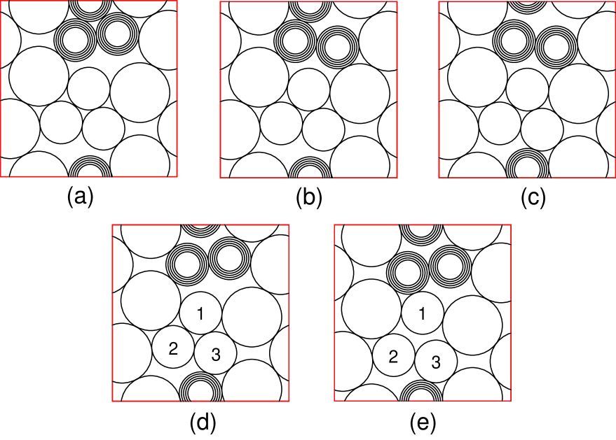
Figure 2: Five distinct collectively jammed states that exist at the same packing fraction $\phi=0.81073$ for a 2d bidisperse system with $N=12$ particles. In (a) through (d), unshaded particles are in the same positions, while the shaded particles are in different locations from panel to panel. Particles labeled $1$, $2$, and $3$ are in different positions in panels (d) and (e), while the other particles are in the same positions.

II Methods

Our goal is to enumerate the collectively jammed configurations in 2d bidisperse systems composed of smooth, repulsive disks. We will focus on bidisperse mixtures composed of $N/2$ large and $N/2$ small particles with a diameter ratio $\eta=1.4$ because it has been shown that these systems do not easily crystallize or phase separate speedy ; ohern_long . We consider system sizes in the range $N=4$ to $256$ particles. For $N\leq 10$, we were able to find nearly all of the collectively jammed states. For $N=12$ ($14$) we found more than $90\%$ ($60\%$) of the total number. Since the number of collectively jammed states grows so rapidly with $N$, we are not able to calculate a large fraction of the CJ states for $N>14$, but as we will show below, we can still make strong conclusions about the shape of the distribution of CJ states in large systems.

We utilize an energy-minimization procedure to create collectively jammed states ohern_long . We assume that the particles interact via the purely repulsive linear spring potential

$$V(r_{ij})=\frac{\epsilon}{2}(1-r_{ij}/d_{ij})^{2}\Theta(d_{ij}/r_{ij}-1),$$ (2)

where $\epsilon$ is the characteristic energy scale, $r_{ij}$ is the separation of particles $i$ and $j$, $d_{ij}=\left(d_{i}+d_{j}\right)/2$ is their average diameter, and $\Theta(x)$ is the Heaviside step function. The potential (2), is nonzero only for $r_{ij}<d_{ij}$, i.e., when the particles overlap. Jammed states are obtained by successively growing or shrinking particles followed by relaxation via potential energy minimization until all particles (excluding floaters) in the system are just at contact. In these prior studies, we showed that the distribution of collectively jammed states does not depend sensitively on the shape of the repulsive potential $V(r_{ij})$. Note that our process for creating jammed states differs from the fixed volume energy minimization procedure implemented in Ref. ohern_long . In the description below, the energies and lengths are measured in units of $\epsilon$ and the diameter of the smaller particle $d_{1}$.

Figure 3: Fraction $f_{\Delta}$ of distinct collectively jammed states with an excess number of contacts $\Delta=N_{c}-N_{c}^{\rm min}$ over a range of system sizes, $N=6$ (circles), $8$ (squares), $10$ (diamonds), $12$ (upward triangles), and $14$ (downward triangles). For $N=6$, all CJ states have $\Delta=0$.

For each independent trial, the procedure begins by choosing a random configuration of $N$ particles at an initial packing fraction $\phi_{i}$ in a square box with unit length and periodic boundary conditions. The positions of the centers of the particles are uncorrelated and distributed uniformly in the box. We have found that the results do not depend on the initial volume fraction $\phi_{i}$ as long it is significantly below the peak in $\rho(\phi)$. We chose $\phi_{i}=0.60$ for most system sizes.

After initializing the systems, we find the nearest local potential energy minimum using the conjugate gradient algorithm numrec . We terminate the energy minimization procedure when either of the following two conditions is satisfied: 1) two successive conjugate gradient steps $n$ and $n+1$ yield nearly the same total potential energy per particle, $(V_{n+1}-V_{n})/V_{n}<\delta=10^{-16}$ or 2) the total potential energy per particle is extremely small, $V_{n+1}<V_{\rm min}=10^{-16}$.

Following the potential energy minimization, we decide whether the system should be compressed or expanded to find the jamming threshold. If $V_{n+1}>V_{\rm max}=2\times 10^{-16}$, particles have nonzero overlap and thus small and large particles are reduced in size by $\Delta d_{1}=d_{1}\Delta\phi/(2\phi)$ and $\Delta d_{2}=\eta\Delta d_{1}$, respectively. If, on the other hand, $V_{n+1}\leq V_{\rm min}$, the system is below the jamming threshold and all particles are thus increased in size. After the system has been expanded or compressed, it is relaxed using potential energy minimization and the process is repeated. Each time the procedure switches from expansion to contraction or vice versa, the packing fraction increment $\Delta\phi$ is reduced by a factor of $2$. The initial expansion rate was $\Delta\phi_{i}=10^{-4}$.

When the total potential energy per particle falls within the range $V_{\rm max}>V>V_{\rm min}$, the process is terminated and the ‘jammed’ packing fraction is recorded. If the final state contains floater particles with $2$ or fewer contacts, we remove them, minimize the total potential energy, and slightly compress or expand the remaining particles to find the jamming threshold. Note that the final configurations are slightly compressed with overlaps in the range $10^{-9}<1-r_{ij}/d_{ij}<10^{-8}$. We have verified that our results do not depend strongly on the parameters $V_{\rm min}$, $V_{\rm max}$, and $\Delta\phi_{i}$.

For each system-size $N$, this process is repeated using $n_{t}^{\prime}$ independent random initial conditions and the resulting jammed configurations are analyzed to determine whether they are collectively jammed and unique.

Figure 4: Fraction of CJ states $n_{s}/n_{s}^{\rm tot}$ versus the ratio of the number of trials $n_{t}$ to the total number of trials $n_{t}^{\rm tot}$ required to find all CJ states $n_{s}^{\rm tot}$ for several system sizes: $N=6$ (dot-dashed), $8$ (dashed), $10$ (thick solid), $12$ (long dashed), and $14$ (dotted). The curves for $N=10$, $12$, and $14$ collapse. The thin solid line is a least-squares fit to Eq. (6). The diamond, upward triangle, and downward triangle symbols give the maximum number of trials attempted for $N=10$, $12$, and $14$, respectively.

III Analysis of Jammed States

To verify if a given final configuration is collectively jammed we analyze the eigenvalue spectra of the dynamical (or rigidity) matrix ohern_long , $M_{i\alpha,j\beta}$, where the indices $i$ and $j$ refer to the particles and $\alpha,\beta=x,y$ represent the Cartesian coordinates. For a system with $N_{f}$ floaters and $N^{\prime}=N-N_{f}$ particles forming a connected network the indices $i$ and $j$ range from $1$ to $N^{\prime}$. Thus, the dynamical matrix has $dN^{\prime}$ rows and columns, where $d=2$ is the spatial dimension. By differentiating the interparticle potential we find that the elements of the dynamical matrix with $i\neq j$ are given by tanguy

$$M_{i\alpha,j\beta}=-\frac{t_{ij}}{r_{ij}}\left(\delta_{\alpha\beta}-{\hat{r}}_{ij\alpha}{\hat{r}}_{ij\beta}\right)-c_{ij}{\hat{r}}_{ij\alpha}{\hat{r}}_{ij\beta},$$ (3)

where $t_{ij}=\partial V/\partial r_{ij}$ and $c_{ij}=\partial^{2}V/\partial r_{ij}^{2}$, while those with $i=j$ are given by

$$M_{i\alpha,i\beta}=-\sum_{j}M_{i\alpha,j\beta}.$$ (4)

The dynamical matrix (3) and (4) has $dN^{\prime}$ real eigenvalues $\{\xi_{i}\}$, $d$ of which are zero due to translational invariance of the system. In a collectively jammed state no set of particle displacements is possible without creating an overlapping configuration; therefore the dynamical matrix has exactly $dN^{\prime}-d$ nonzero eigenvalues. In our simulations we use the criterion $|\xi_{i}|>\xi_{\rm min}$ for nonzero eigenvalues, where $\xi_{\rm min}=10^{-6}$ is the noise threshold for our eigenvalue calculations.

We note that our energy minimization algorithm for creating jammed states does occasionally yield a configuration that is not collectively jammed. These states, however, are not considered in the current study. The number of trials that yield collectively jammed states out of the original $n_{t}^{\prime}$ trials is denoted $n_{t}$. The fraction of trials that give locally but not collectively jammed states $(n_{t}^{\prime}-n_{t})/n_{t}^{\prime}$ decreases with increasing system size from $\approx 5\%$ at $N=6$ to less than $1\%$ for $N>12$.

Figure 5: The total number of distinct CJ states $n_{s}^{\rm tot}$ (circles) and the number of trials required to find them (squares) versus system-size $N$. The solid and dotted lines have slopes equal to $1.2$ and $1.7$, respectively.

We determine whether two collectively jammed states are distinct by comparing the sorted lists of the nonzero eigenvalues of their respective dynamical matrices. If the relative difference between two corresponding eigenvalues differs by more than $\xi_{\rm diff}=10^{-3}$, the configurations are treated as distinct. By comparing the topology of the network of particle contacts in a representative sample of CJ states, we have found that this criterion is sufficient to reliably determine whether two states are distinct or identical.

This procedure allows us to determine the number $n_{s}$ of distinct collectively jammed states at each fixed number of independent trials $n_{t}$. As expected, if two CJ states have different packing fractions, they are distinct, with different contact networks and dynamical modes. This property holds with very high numerical precision—the packing-fraction difference of $10^{-13}$ already assures that the two states are distinct.

However, it is not true that all collectively jammed states with the same packing fraction are identical. For example, the CJ states shown in Fig. 2 have the same packing fraction, but they possess different contact networks and eigenvalue spectra. This is a clear demonstration that two collectively jammed configurations at the same packing fraction can have very different structural properties.

We have also calculated the total number of contacts between particles $N_{c}$, i.e. the number of bonds that satisfy $r_{ij}<d_{ij}$, in our slightly compressed jammed configurations. We find that the number of contacts in the collectively jammed states satisfies the relation zinchenko ; donev_2005

$$N_{c}\geq N_{c}^{\rm min}=2\left(dN^{\prime}-d+1\right).$$ (5)

The minimum number of contacts required for mechanical stability of the system $N_{c}^{\rm min}$ can be calculated by equating the number of degrees of freedom to the number of constraints. Note that an extra constraint is required to prevent particle expansion. We have found that nearly all of the collectively jammed states have $N_{c}=N_{c}^{\rm min}$; fewer than $1\%$ of these states have $N_{c}>N_{c}^{\rm min}$ as shown in Fig. 3. All configurations that are not collectively jammed have fewer contacts than $N_{c}^{\rm min}$.

Table 1: Maximum number of trials performed $n_{t}^{\rm max}$ and fraction of CJ states obtained $(n_{s}/n_{s}^{\rm tot})_{\rm max}$ versus system size $N$.

$N$		$n_{t}^{\rm max}$	$(n_{s}/n_{s}^{\rm tot})_{\rm max}$
$6$		$10^{6}$	$1.0$
$8$		$10^{6}$	$1.0$
$10$		$29\times 10^{6}$	$1.0$
$12$		$28\times 10^{6}$	$0.90$
$14$		$26\times 10^{6}$	$0.60$

IV Results

In the preceding two sections, we described our methods for generating and counting distinct collectively jammed states. We will now present the results from these analyses. We will first discuss how the number of CJ states depends on parameters such as the number of trials and system size. We then decompose the probability density of obtaining a CJ state at a given packing fraction (Eq. (1)) into the density $\rho(\phi)$ of CJ packing fractions and their frequency distribution $\beta(\phi)$. We also consider under what conditions all of the possible CJ states can be enumerated and determine whether strong conclusions can be made about the distributions of CJ states in large systems even though complete enumeration is not possible.

Figure 6: Probability distribution $P(\phi)$ for obtaining a CJ state at $\phi$ for $N=10$ (solid line) and $N=14$ (dotted line) at $(n_{s}/n_{s}^{\rm tot})_{\rm max}$. The distributions at $n_{s}/n_{s}^{\rm tot}=0.05$ (squares for $N=10$ and triangles for $N=14$) overlap those with larger $n_{s}/n_{s}^{\rm tot}$.

Our studies of the number of distinct CJ states $n_{s}$ versus the number of independent trials $n_{t}$ led to several surprising observations. First, we find that these systems possess a significant fraction of rare CJ states and thus an exponentially large number of trials are required to obtain nearly all states. Second, a master curve appears to describe $n_{s}(n_{t})$ for systems with $N\geq 10$, as shown in Fig. 4. (Each data point in this figure was obtained by averaging over at least $100$ distinct permutations of the $n_{t}$ trials.) Our numerical results indicate that when $n_{s}$ is more than about $20\%$ of the total number of distinct CJ states $n_{s}^{\rm tot}$, the curve $n_{s}(n_{t})$ can be accurately approximated by

$$\frac{n_{s}}{n_{s}^{\rm tot}}=1-A\left[\log_{10}\left(\frac{n_{t}}{n_{t}^{\rm tot}}\right)\right]^{2},$$ (6)

where $A\approx 0.05$.

Our direct computations for small systems ($N=6$, $8$, and $10$) and numerical fits to the master curve (6) for $N=12$ and $14$ indicate that both $n_{t}^{\rm tot}$ and $n_{s}^{\rm tot}$ increase exponentially with system size as shown in Fig. 5. However, both these quantities remain finite for any finite system. In particular, for the smallest system sizes, we increased the total number of trials by at least a factor of $10$ and did not find any new collectively jammed states. We also used several different algorithms for generating CJ states, e.g. compression and expansion of particles followed by relaxation using molecular dynamics with dissipative forces along ${\hat{r}}_{ij}$ and frictional forces perpendicular to ${\hat{r}}_{ij}$, and these did not lead to any new CJ states that were not already found using the protocol described in Sec. II. The maximum number of trials and fraction of CJ states obtained are provided in Table 1.

Figure 7: Density of collectively jammed packing fractions $\rho(\phi)$ for (a) $N=10$, (b) $12$, and (c) $14$ at $n_{s}/n_{s}^{\rm tot}=0.2$ (solid), $0.4$ (dotted), $0.6$ (dot-dashed), $0.8$ (long-dashed), and $1.0$ (dashed).

As indicated in Eq. (1), the probability distribution $P(\phi)$ for obtaining a collectively jammed state at a particular packing fraction $\phi$ can be factorized into two composite functions: the density of CJ states $\rho(\phi)$ and the frequency $\beta(\phi)$ with which these states occur. In our simulations, the distribution $P(\phi)$ is calculated from the relation

$$P(\phi)d\phi=\frac{n_{P}(\phi+d\phi)-n_{P}(\phi)}{n_{t}}.$$ (7)

Here $n_{P}(\phi)$ is the total number of CJ states (counting all repetitions of the same state) with packing fractions below $\phi$. The density of CJ states is evaluated using an analogous relation

$$\rho(\phi)d\phi=\frac{n_{s}(\phi+d\phi)-n_{s}(\phi)}{n_{s}},$$ (8)

where $n_{s}(\phi)$ is the number of distinct CJ states that have been detected in the packing-fraction range below $\phi$. (In fact, we have used the number of distinct packing fractions to define $\rho(\phi)$ in place of the number of distinct CJ states $n_{s}(\phi)$. However, this does not affect our results because distinct states with the same $\phi$ are rare in 2d bidisperse systems.) We note that both the probability density (7) and the density of CJ states (8) are normalized to 1. The frequency distribution $\beta(\phi)=P(\phi)/\rho(\phi)$ is normalized accordingly.

Below, we show how $P(\phi)$, $\rho(\phi)$, and $\beta(\phi)$ depend on the fraction of CJ states $n_{s}/n_{s}^{\rm tot}$ and system size $N$. To plot these distributions, we used $10$ bins with the endpoint of the final bin located at the largest CJ packing fraction $\phi_{\rm max}$ for each $N$. We recall that the distribution of CJ packing fractions $\rho(\phi)$ does not depend on the protocol used to generate the CJ states. The protocol dependence of the distribution $P(\phi)$ is captured by the frequency distribution $\beta(\phi)$.

The probability distribution $P(\phi)$ of CJ states is shown in Fig. 6 for two small systems $N=10$ and $14$. The results indicate that $P(\phi)$ depends very weakly on the fraction $n_{s}/n_{s}^{\rm tot}$ of CJ states obtained—only $5\%$ of the CJ states are required to capture accurately the shape of $P(\phi)$ for these systems. This result holds for all system sizes we studied, which implies that the distribution of CJ states can be measured reliably even in large systems ohern_long ; ohern_short . Note that the width and the location of the peak in $P(\phi)$ do not change markedly over the narrow range of $N$ shown in Fig. 6.

To see significant changes in $P(\phi)$, the system size must be varied over a larger range. $P(\phi)$ for $N=18$, $32$, $64$, and $256$ are shown in Fig. 1 at fixed number of trials $n_{t}=10^{4}$. The width of the distribution narrows and the peak position shifts to larger $\phi$ as the system size increases. In Ref. ohern_long , we found that $P(\phi)$ for this 2d bidisperse system becomes a $\delta$-function located at $\phi_{0}=0.842$ in the infinite-system-size limit. What causes $P(\phi)$ to narrow to a $\delta$-function located at $\phi_{0}$ when $N\rightarrow\infty$? Is the shape of the distribution $P(\phi)$ determined primarily by the density of states $\rho(\phi)$, or does the frequency distribution $\beta(\phi)$ play a significant role in determining the width and location of the peak? We will shed light on these questions below.

Figure 8: Density of collectively jammed packing fractions $\rho(\phi)$ for $N=8$ (solid), $10$ (dotted), $12$ (dot-dashed), and $14$ (long-dashed) at $(n_{s}/n_{s}^{tot})_{\rm max}$.

We first show results for $\rho(\phi)$ and $\beta(\phi)$ as functions of the fraction $n_{s}/n_{s}^{\rm tot}$ of distinct CJ states obtained. In Fig. 7, $\rho(\phi)$ is shown for several small systems. In contrast to the total distribution $P(\phi)$, the density of states $\rho(\phi)$ depends on $n_{s}/n_{s}^{\rm tot}$ significantly. For $N=10$, a system for which we can calculate nearly all of the CJ states, the curve $\rho(\phi)$ reaches its final height and width when $n_{s}/n_{s}^{\rm tot}\approx 0.5$. However, its shape still slowly evolves as $n_{s}/n_{s}^{\rm tot}$ increases above $0.5$; the low-$\phi$ part of the curve increases while the high-$\phi$ side decreases. This implies that the rare CJ states are not uniformly distributed in $\phi$, but are more likely to occur at low packing fractions below the peak in $\rho(\phi)$. Similar results for $\rho(\phi)$ as functions of $n_{s}/n_{s}^{\rm tot}$ are found for $N=12$ and $14$. By comparing $\rho(\phi)$ at fixed $n_{s}/n_{s}^{tot}$, we also find that $\rho(\phi)$ narrows with increasing $N$. To further demonstrate that $\rho(\phi)$ narrows, the density of states is plotted in Fig. 8 for several system sizes at $(n_{s}/n_{s}^{\rm tot})_{\rm max}$ listed in Table 1.

Figure 9: Frequency distribution $\beta(\phi)$ for (a) $N=10$, (b) $12$, and (c) $14$ for $n_{s}/n_{s}^{\rm tot}=0.2$ (solid), $0.4$ (dotted), $0.6$ (dot-dashed), $0.8$ (long-dashed), and $1.0$ (dashed).

The dependence of the frequency distribution $\beta(\phi)$ on the system size $N$ and the fraction $n_{s}/n_{s}^{\rm tot}$ of CJ states obtained is illustrated in Fig. 9. The results show that in contrast to the functions $P(\phi)$ and $\rho(\phi)$, the distribution $\beta(\phi)$ achieves its maximal value at the highest packing fraction for which CJ states exist $\phi_{\rm max}$. By comparing $\beta(\phi)$ for different system sizes at fixed $n_{s}/n_{s}^{\rm tot}$ we find that $\phi_{max}$ increases with increasing $N$.

The frequency distribution $\beta(\phi)$ becomes more strongly peaked at $\phi_{\max}$ as $n_{s}/n_{s}^{\rm tot}$ increases. The evolution of $\beta(\phi)$ with $n_{s}/n_{s}^{\rm tot}$ can be explained by noting that $\beta(\phi)\equiv P(\phi)/\rho(\phi)$ and that $P(\phi)$ does not depend on $n_{s}/n_{s}^{\rm tot}$ for $n_{s}/n_{s}^{\rm tot}\gtrsim 0.05$ according to the results shown in Fig. 6. The density of states $\rho(\phi)$ and the frequency distribution $\beta(\phi)$ must therefore behave in opposite ways to maintain constant $P(\phi)$. As shown earlier in Fig. 7, the peak in $\rho(\phi)$ widens (for $n_{s}/n_{s}^{\rm tot}<0.5$) and shifts to lower packing fractions as $n_{s}/n_{s}^{\rm tot}$ increases. Thus, the distribution $\beta(\phi)$ must decrease at low packing fractions and build up at large packing fractions with increasing $n_{s}/n_{s}^{\rm tot}$.

Figure 10: Frequency distribution $\beta_{n}(\phi)$ normalized by the peak value for (a) $N=10$, (b) $N=12$, and (c) $N=14$ at $n_{s}/n_{s}^{\rm tot}=0.2$ (solid), $0.4$ (dotted), $0.6$ (dot-dashed), $0.8$ (long-dashed), and $1.0$ (dashed). Least squares fits to exponential curves (thin solid lines) are also shown for the largest $n_{s}/n_{s}^{\rm tot}$ at each $N$.

In Fig. 10, we show the frequency distribution $\beta_{n}(\phi)=\beta(\phi)/\beta_{\rm max}$, which is normalized by the peak value $\beta_{\rm max}$. The results are plotted on a logarithmic scale. The frequency distribution varies strongly with $\phi$; CJ states with small packing fractions are rare and those with large packing fractions $(\phi\approx 0.83)$ occur frequently. We find that $\beta_{n}(\phi)$ is exponential over an expanding range of $\phi$ as $n_{s}/n_{s}^{\rm tot}$ increases. For $N=10$, $\beta_{n}(\phi)$ increases exponentially over nearly the entire range of $\phi$ at $n_{s}/n_{s}^{\rm tot}=1$. We see similar behavior for $N=12$ and $14$ in panels (b) and (c) of Fig. 10; thus we expect $\beta_{n}(\phi)$ to be exponential as $N_{s}/N_{s}^{\rm tot}\rightarrow 1$ for $N>10$. We have calculated least-squares fits to

$$\beta_{n}=A_{\beta}\exp(B_{\beta}\phi)$$ (9)

for the largest $n_{s}/n_{s}^{tot}$ at each system size. As pointed out above, the frequency distribution becomes steeper with increasing $N$; we find that $B_{\beta}$ increases by a factor of $3.5$ as $N$ increases from $10$ to $18$ (not shown). Note that reasonable estimates of $B_{\beta}$ can be obtained even at fairly low values of $n_{s}/n_{s}^{\rm tot}$.

Figure 11: Cumulative probability distribution $F_{h}$ of CJ states in a narrow range of packing fractions $d\phi$ for N=12. The index $i$ denotes the position of the state in a list ordered by the frequency of occurrence and $n_{s}$ is the total number of states in the given interval. The solid lines correspond to bins centered on $\phi=0.73$, $0.75$, $0.77$, and $0.79$; the dashed lines labeled $1$, $2$, $3$, and $4$ correspond to bins centered on $\phi=0.65$, $0.81$, $0.83$, and $0.69$, respectively. The width of each bin is $\Delta\phi=0.02$. The inset shows that the data are well-described by Eq. (10), where $A_{F}\approx 2.4$ and $\alpha$ varies from $0.3$ to $0.4$.

We showed in Fig. 10 that the frequency distribution is not uniform in $\phi$; in contrast, it increases exponentially with $\phi$. Fig. 11 shows another striking result; the frequency distribution is also highly nonuniform within a narrow range of $\phi$. In this figure, we plot the cumulative distribution $F_{h}$ of the probabilities of jammed states in an narrow interval $d\phi$ versus the index $i$ in a list of all distinct states in $d\phi$ ordered by the value of the probability of each state. The data for several different intervals appear to collapse onto a stretched exponential form,

$$F_{h}=\exp\left[-A_{F}\left(1-i/n_{s}\right)^{\alpha}\right],$$ (10)

where $n_{s}$ is the number of distinct CJ states within $d\phi$ and the exponent $\alpha$ varies from $0.3$ to $0.4$. These results clearly demonstrate that CJ states can occur with very different frequencies even if they have similar packing fractions.

From our studies of small systems, we find that both the density $\rho(\phi)$ of CJ packing fractions and the frequency distribution $\beta(\phi)$ narrow and shift to larger packing fractions as the system size increases. (See Figs. 7 and  10.) How do these changes in $\rho(\phi)$ and $\beta(\phi)$ affect the total distribution $P(\phi)$ and can we determine which changes dominate in the large system limit? To shed some light on these questions, we consider the position of the peak in $P(\phi)$ with respect to the maximal packing fraction of CJ states $\phi_{\rm max}$ for several system sizes. In the absence of changes in $\rho(\phi)$ as a function of $\phi-\phi_{\rm max}$, the maximum of $P(\phi)$ should shift toward $\phi=\phi_{\rm\max}$ with increasing system size, because the frequency distribution $\beta$ becomes more sharply peaked at $\phi_{\rm max}$ according to the results in Fig. 10. However, as shown in Fig. 12, we find the opposite behavior over the range of system sizes we considered: the peak of $P(\phi)$ shifts away from $\phi_{\max}$. This suggests that the density of states, not the frequency distribution, plays a larger role in determining the location of the peak in $P(\phi)$ in these systems.

Additional conclusions about the relative roles of the the density of states and the frequency distribution on the position and width of $P(\phi)$ can be drawn from our observation that the frequency distribution $\beta$ is an exponential function of $\phi$ (c.f. the discussion of results in Fig. 10) and that $P(\phi)$ is Gaussian for sufficiently large systems (as shown in ohern_long and illustrated in Fig. 13). If we assume that the exponential form of the frequency distribution (9) remains valid in the large-system-limit, the density of states $\rho(\phi)=P(\phi)/\beta(\phi)$ is also Gaussian with the identical width $\sigma(N)$. The location of the peak in $P(\phi)$ is

$$\phi^{*}_{P}(N)=\phi^{*}_{\rho}(N)+B_{\beta}(N)\sigma(N),$$ (11)

where $\phi_{\rho}^{*}(N)$ is the location of the peak in $\rho(\phi)$. In previous studies ohern_long , we found that the width of $P(\phi)$ scaled as $\sigma\sim N^{-\Omega}$, with $\Omega\approx 0.55$. We have also some indication that $B_{\beta}\sigma^{2}$ decreases with increasing system size: $B_{\beta}\sigma^{2}=0.017$ at $N=12$ compared to $0.012$ at $N=18$. However, we are not currently able to estimate $B_{\beta}$ in the large $N$ limit.

Figure 12: $P(\phi^{\prime})$ (thick lines) and $\beta_{n}(\phi^{\prime})$ (thin lines) for $N=10$ (solid), $12$ (dotted), and $N=14$ (dot-dashed) at $(n_{s}/n_{s}^{tot})_{\rm max}$, where $\phi^{\prime}=\phi+\Delta\phi$. $P(\phi)$ and $\beta_{n}(\phi)$ for $N=10$, $12$, and $14$ have been shifted by $\Delta\phi=0.013$, $0.005$, and $0$ respectively, so that $\beta_{\rm max}$ for the three system sizes coincide. $\beta_{n}(\phi)$ for each $N$ has also been amplified by a factor of $\approx 20$.

If the system-size dependence of $B_{\beta}$ is weaker than $N^{2\Omega}$, the quantity $B_{\beta}\sigma^{2}$ will tend to zero and the frequency distribution will not influence the location of the peak in $P(\phi)$. In this case $P(\phi)$ becomes independent of the frequency distribution in the limit $N\to\infty$ for a class of protocols that are characterized by a similar frequency distribution $\beta$ as our present protocol. Thus, as our preliminary results suggest, random close packing can be defined as the location of the peak in $\rho(\phi)$ when $N\rightarrow\infty$, and this definition is completely independent of on the algorithm used to generate the CJ states. In the opposite case, where the system-size dependence of $B_{\beta}$ is stronger than $N^{2\Omega}$, the position of the peak in $P(\phi)$ results from a subtle interplay between the density of states and the frequency distribution. However, even in this case one can argue that the dependence of the position of the peak only weakly depends on the protocol: a shift of the peak position requires an exponential change in the frequency distribution $\beta(\phi)$.

Figure 13: The distribution $P(\phi)$ of CJ states for (a) $N=18$, (b) $32$, (c) $64$, and (d) $256$ are depicted using circles. The solid lines are least squares fits of the large-$\phi$ side of $P(\phi)$ to Gaussian distributions.

V Conclusions

We have studied the possible collectively jammed configurations that occur in small 2d periodic systems composed of smooth purely repulsive bidisperse disks. The CJ states were created by successively compressing or expanding soft particles and minimizing the total energy at each step until the particles were just at contact. By studying small 2d systems, we were able to enumerate nearly all of the collectively jammed states at each system size and therefore decompose the probability distribution $P(\phi)$ for obtaining a CJ state at a particular packing fraction $\phi$ into the density $\rho(\phi)$ of CJ packing fractions and their frequency distribution $\beta(\phi)$. The distribution $\beta(\phi)$ depends on the particular protocol used to generate the CJ configurations, while $\rho(\phi)$ does not. This decomposition allowed us to study how the protocol-independent $\rho(\phi)$ and protocol-dependent $\beta(\phi)$ influence the shape of $P(\phi)$.

These studies yielded many important and novel results. First, the probability distribution $P(\phi)$ of CJ states is nearly independent of $n_{s}/n_{s}^{\rm tot}$, and thus it can be measured reliably even in large systems. This finding validates several previous measurements of $P(\phi)$ ohern_long ; ohern_short . Second, the number of distinct CJ states grows exponentially with system size. In addition, a large fraction of these configurations are extremely rare and thus an exponentially large number of trials are required to find all of the CJ states. Third, the frequency distribution $\beta(\phi)$ are nonuniform and increase exponentially with $\phi$. We also found that even over a narrow range of $\phi$, the frequency with which particular CJ states occur is strongly nonuniform and involves a large number of exponentially rare states. Finally, we have shown that $P(\phi)$ becomes Gaussian in the large $N$ limit. Since $P(\phi)=\rho(\phi)\beta(\phi)$ and $\beta(\phi)$ is exponential, we expect that $\rho(\phi)$ is also Gaussian and controls the width of $P(\phi)$ for large $N$. We also have preliminary results that suggest that the contribution from $\beta(\phi)$ to the shift of the peak in $P(\phi)$ decreases with increasing $N$. We expect that $\rho(\phi)$ will determine the location of the peak in $P(\phi)$ in the large $N$ limit, and thus it is a robust protocol-independent definition of random close packing in this system.

VI Future Directions

Several interesting questions have arisen from this work that will be addressed in our future studies. First, we have shown that the frequency with which CJ states occur is highly nonuniform. It is important to ask whether the rare states can be neglected in analyses of static and dynamic properties of jammed and nearly jammed systems. For example, we have shown that $P(\phi)$ is insensitive to the fraction $n_{s}/n_{s}^{\rm tot}$ of CJ states obtained and thus $P(\phi)$ is not influenced by the rare CJ states. However, rare CJ states may be important in determining the dynamical properties of jammed and glassy systems if these states are associated with ‘passages’ or ‘channels’ from one frequently occurring state to another. Moreover, an analysis of the density of states and the frequency distribution (both as a function of $\phi$ and locally in $\phi)$ may shed light on the phase space evolution of glassy systems during the aging process.

A closely related question is what topological or geometrical features of configurational phase space give rise to the exponentially varying frequency distribution? Can one, for example, uniquely assign a specific volume in configurational space to each jammed state? A candidate for such a quantity is the volume $\Omega_{c}$ of configuration space in which each point is connected by a continuous path without particle overlap to a particular CJ state. It is likely that those CJ states with large $\Omega_{c}$ will occur frequently for a typical compaction algorithm, while those with small $\Omega_{c}$ will be rare.

Figure 14: $P(\phi)$ (solid), $\rho(\phi)$ (dotted), and $\beta(\phi)$ (dot-dashed) for a 2d monodisperse system with $N=24$.

Another important question is whether the results for $\rho(\phi)$, $\beta(\phi)$, and $P(\phi)$ found in 2d bidisperse systems also hold for other systems such as monodisperse systems in 2d and 3d. Does $\rho(\phi)$ still control the behavior of $P(\phi)$ or does the frequency distribution play a more dominant role in determining $P(\phi)$? To begin to address these questions, we have enumerated nearly all of the distinct collectively jammed states and calculated $P(\phi)$, $\rho(\phi)$, and $\beta(\phi)$ in small 2d periodic cells containing $N=4$ to $32$ equal-sized particles.

In our preliminary studies, we have found several significant differences between 2d monodisperse and bidisperse systems, which largely stem from the fact that partially ordered states occur frequently in the monodisperse systems. First, in 2d monodisperse systems there is an abundance of distinct CJ states that exist at the same packing fraction. For example, in a monodisperse systems with $N=24$, multiple distinct states occur at $19\%$ of the CJ packing fractions compared to less than $1\%$ in bidisperse systems with $N=14$. Second, for the system sizes studied, quantitative features of the distributions of CJ states depend on whether $N$ is even or odd. Third, $P(\phi)$ can possess two strong peaks. For example, two peaks in $P(\phi)$ occur at $\phi_{1}\approx 0.805$ and $\phi_{2}\approx 0.844$ for $N=24$ as shown in Fig. 14. Moreover, the large-$\phi$ peak that corresponds to partially ordered configurations is a factor of three taller than the small-$\phi$ peak that corresponds to amorphous configurations. Finally, the maximum in $\beta(\phi)$ coincides with the large-$\phi$ peak in $P(\phi)$ and $\beta(\phi)$ decays very rapidly as $\phi$ decreases. As shown in Fig. 14, the rapid decay of $\beta(\phi)$ significantly suppresses the contribution of the peak in $\rho(\phi)$ to the total distribution $P(\phi)$. Thus, $\beta(\phi)$, which depends on the protocol used to generate the CJ states, may strongly influence the total distribution $P(\phi)$ even in moderately sized 2d monodisperse systems.

Many open questions concerning monodisperse systems in 2d will be answered in a forthcoming article ning . We will measure the shape of $P(\phi)$ as a function of system size and predict whether $\rho(\phi)$ or $\beta(\phi)$ controls the width and location of the peak (or peaks) in the large $N$ limit. The fact that $\beta(\phi)$ strongly influences $P(\phi)$ at small and moderate system sizes explains why it has been so difficult to determine random close packing in 2d monodisperse systems berryman —different protocols have yielded different values for $\phi_{\rm rcp}$ torquato_2000 ; donev .

Acknowledgments

Financial support from NSF grant numbers CTS-0348175 (JB) and DMR-0448838 (NX,CSO) is gratefully acknowledged. We also thank Yale’s High Performance Computing Center for generous amounts of computer time.

References

- (1) Jamming and Rheology ed. A. J. Liu and S. R. Nagel (Taylor & Francis, N. Y., 2001).
- (2) J. D. Bernal, Nature 188, 910 (1960).
- (3) G. D. Scott, Nature 188, 908 (1960).
- (4) J. B. Knight, C. G. Fandrich, C. N. Lau, H. M. Jaeger, and S. R. Nagel, Phys. Rev. E 51, 3957 (1995).
- (5) P. Phillippe and D. Bideau, Europhys. Lett., 60, 677 (2002).
- (6) R. P. A. Dullens and W. K. Kegel, Phys. Rev. Lett. 92, 195702 (2004).
- (7) J. X. Zhu, M. Li, R. Rogers, W. Meyer, R. H. Ottewill, W. B. Russell, and P. M. Chaikin, Nature 387, 883 (1997).
- (8) J. L. Finney, Proc. Roy. Soc. Lond. A 319, 495 (1970).
- (9) B. D. Lubachevsky, F. H. Stillinger, and E. N. Pinson, J. Stat. Phys. 64, 501 (1991); B. D. Lubachevsky, J. Comput. Phys. 94, 255 (1991).
- (10) A. Pavlovitch, R. Jullien, and P. Meakin, Physica A 176, 206 (1991).
- (11) A. V. Tkachenko and T. A. Witten, Phys. Rev. E 60, 687 (1999).
- (12) G. C. Barker and M. J. Grimson, J. Phys.: Condens. Matter 1, 2779 (1989).
- (13) W. S. Jodrey and E. M. Tory, Phys. Rev. A 32, 2347 (1985).
- (14) A. S. Clarke and J. D. Wiley, Phys. Rev. B 35, 7350 (1987).
- (15) R. J. Speedy, J. Phys.: Condens. Matter 10, 4185 (1998).
- (16) C. S. O’Hern, L. E. Silbert, A. J. Liu, and S. R. Nagel, Phys. Rev. E 68, 011306 (2003).
- (17) A. Z. Zinchenko, J. Comput. Phys. 114, 298 (1994).
- (18) J. G. Berryman, Phys. Rev. A 27, 1053 (1983).
- (19) C. S. O’Hern, S. A. Langer, A. J. Liu, and S. R. Nagel, Phys. Rev. Lett. 88, 075507 (2002).
- (20) S. Torquato, T. M. Truskett, and P. G. Debenedetti, Phys. Rev. Lett. 84, 2064 (2000).
- (21) S. Torquato and F. H. Stillinger, J. Phys. Chem. B 105, 11849 (2001).
- (22) R. J. Speedy, J. Chem. Phys. 110, 4559 (1999).
- (23) R. K. Bowles and R. J. Speedy, Physica A 262, 76 (1999).
- (24) W. H. Press, B. P. Flannery, S. A. Teukolsky, and W. T. Vetterling, Numerical Recipes in Fortran 77 (Cambridge University Press, New York, 1986).
- (25) A. Tanguy, J. P. Wittmer, F. Leonforte, and J.-L. Barrat, Phys. Rev. B 66, 174205 (2002).
- (26) A. Donev, S. Torquato, and F. H. Stillinger, Phys. Rev. E 71, 011105 (2005).
- (27) N. Xu, J. Blawzdziewicz, and C. S. O’Hern (unpublished).
- (28) A. Donev, S. Torquato, F. H. Stillinger, and R. Connelly, J. Applied Phys. 95, 989 (2004).