Reduction of Two-Dimensional Dilute Ising Spin Glasses

Abstract

The recently proposed reduction method is applied to the Edwards-Anderson model on bond-diluted square lattices. This allows, in combination with a graph-theoretical matching algorithm, to calculate numerically exact ground states of large systems. Low-temperature domain-wall excitations are studied to determine the stiffness exponent $y_{2}$. A value of $y_{2}=-0.281(3)$ is found, consistent with previous results obtained on undiluted lattices. This comparison demonstrates the validity of the reduction method for bond-diluted spin systems and provides strong support for similar studies proclaiming accurate results for stiffness exponents in dimensions $d=3,\ldots,7$. PACS number(s): 05.50.+q, 64.60.Cn, 75.10.Nr, 02.60.Pn.

I Introduction

Despite more than two decades of intensive research, many properties of spin glasses reviewSG1 ; reviewSG2 ; F+H ; reviewSG3 , especially in finite dimensions, are still not well understood. The most simple model is the Edwards-Anderson model (EA) F+H ,

$$H=-\sum_{<i,j>}\,J_{i,j}\,x_{i}\,x_{j},\quad(x_{i}=\pm 1),$$ (1)

with Ising spins $x_{i}=\pm 1$ arranged on a finite-dimensional lattice with nearest-neighbor bonds $J_{i,j}$, randomly drawn from a distribution $P(J)$ of zero mean and unit variance.

For two-dimensional Ising spin glasses it is now widely accepted that no ordered phase for finite temperatures exists RSBDJ ; kawashima1997 ; HY ; houdayer2001 ; AMMP , while spin glasses order at low temperatures in higher dimensions kawashima1996 ; marinari1998 ; Hy3d ; CBM . This can be seen e.g. by studying the stiffness exponent $y$ (often labeled $\theta$) which is in many respects one of the most fundamental quantities to characterize the low-temperature state of disordered systems. This exponent provides an insight into the effect of low-energy excitations of such a system FH ; BM1 . A recent study suggested the importance of this exponent for the scaling corrections of many observables in the low-temperature regime BKM , and it is an essential ingredient to understand the true nature of the energy landscape of finite-dimensional glasses KM ; PY2 ; PY .

To illustrate the meaning of the stiffness exponent, one my consider an ordinary Ising ferromagnet of size $L^{d}$ having bonds $J=+1$, which is well-ordered at $T=0$ for $d>1$, with periodic boundary conditions. If we make the boundary along one spatial direction anti-periodic, the system would form an interface of violated bonds between mis-aligned spins, which would raise the energy of the system by $\Delta E\sim L^{d-1}$. This “defect”-energy $\Delta E$ provides a measure for the energetic cost of growing a domain of overturned spins, which in a ferromagnet simply scales with the surface of the domain. In a disordered system, say, a spin glass with an equal mix of $J=\pm 1$ couplings, the interface of such a growing domain can take advantage of already-frustrated bonds to grow at a reduced or even decreasing cost. To wit, we measure the probability distribution $P(\Delta E)$ of the interface energies induced by perturbations at the boundary of size $L$, for which the typical range $\sigma(\Delta E)=\sqrt{<\Delta E^{2}>-<\Delta E>^{2}}$ of the defect-energy may scale like

$$\sigma(\Delta E)\sim\,L^{y}.$$ (2)

From the above consideration it is clear that $y\leq d-1$, and a bound of $y\leq(d-1)/2$ has been proposed for the Edwards-Anderson model generally FH . Particular ground states of systems with $y\leq 0$ would be unstable or only marginally stable with respect to spontaneous fluctuations, whether induced thermally or structurally. These fluctuations could grow at no cost, like in the case of the one-dimensional ferromagnet where $y=d-1=0$. Such a system does not manage to attain an ordered state for any finite temperature. Conversely, a positive sign for $y$ at $T=0$ indicates a finite-temperature transition into an ordered regime while its value is a measure of the stability of the ordered state. It is generally believed that the EA possesses a glassy low-temperature regime, i. e. $y>0$, for $d\geq 3$ PY ; SY ; Kirkpatrick ; Hy3d ; CBM ; BM ; BC ; CB ; MKpaper ; Hd4 ; hukushima2000 , while such a phase is absent, and $y<0$, for $d\leq 2$ HY ; AMMP ; BM ; HBCMY . A value of $y=0$ marks the lower critical dimension.

The stiffness exponent provides a measure of the effect of excitations on a spin system around ground state configurations, induced by low-temperature fluctuations. It is computationally convenient to induce such excitations by perturbing the system of size $n=L^{d}$ at one boundary and measuring the response for increasing system size $L$. The square lattices considered here have one open and one periodic boundary, and we determine the energy difference $\Delta E$ between the ground states of a given bond-configuration, once with periodic and once with anti-periodic boundary conditions (P-AP method). Anti-periodic boundary conditions are obtained by reversing the sign of a strip of bonds along the periodic boundary. Using a symmetric bond distribution $P(J)$, $\Delta E$ will be also symmetrically distributed, but with a variance $\sigma$ of these excitation that may scale with $L$ according to Eq. (2).

Until recently, the consensus of the results for $d=3$ ranged from $y_{3}\approx 0.19$ to $\approx 0.27$ PY ; SY ; Kirkpatrick ; BC ; BM ; CB ; Hy3d ; CBM ; MKpaper , while there was only two results in $d=4$, $y_{4}=0.64(5)$ Hd4 and $y_{4}=0.82(6)$ hukushima2000 . In Refs. Stiff1 ; Stiff2 , it was proposed to study the EA in Eq. (1) on bond-diluted lattices to obtain more accurate scaling behavior for low-temperature excitations. One can remove iteratively low-connected spins from the lattice and alter the interactions, i.e. reduce the system, in such a way that the ground-state energy of the reduced system is the same as the original system. In this way often much larger lattice sizes $L$ can be simulated compared to undiluted ones and, in combination with finite-size scaling, enhanced scaling regimes are achieved. In this manner, improved or entirely new values for the $T=0$ stiffness exponents in dimensions $d=3$ to 7 were computed for lattices with discrete bonds, $\pm J$, resulting in $y_{3}=0.24(1)$, $y_{4}=0.61(2)$, $y_{5}=0.88(5)$, $y_{6}=1.1(1)$, and $y_{7}=1.24(5)$.

The novelty of the procedure used in Refs. Stiff1 ; Stiff2 makes it difficult to assess the validity and the accuracy of the approach, since few data of comparable accuracy exists for the results presented there. The scaling Ansatz used is based on various reasonable but untested assumptions, for instance that the stiffness exponent does not depend on the dilution. Therefore, this approach has been discussed in the context of the Migdal-Kadanoff approximation BoCo to justify the scaling Ansatz. Here, we apply this procedure to the EA in $d=2$, which has been studied extensively in recent years. These studies have found the value of the stiffness exponent $y$ to be $y_{2}=-0.281(2)$ RSBDJ , $y_{2}=0.287(4)$ HBCMY , or $y_{2}=-0.282(2)$ HY ; CBM . We find that the result obtained here on diluted lattices, $y_{2}=-0.281(3)$, compares well with those earlier results. This does not add any accuracy to the value of $y_{2}$, and we find anew BoCo that diluted lattices with continuous (Gaussian) bonds are beset with more complex scaling behavior BF as well as more extensive scaling corrections. Much more important, though, the present study indicates the correctness of the reduction approach, hence the validity of the results obtained for larger dimensions. In particular, the stiffness exponent does not depend on the dilution, i.e. it is universal, even when $y<0$.

In the next section, we describe the algorithm we applied to reduce and evaluate large instances of dilute, planar lattices and outline the ground-state algorithm. In Sec. IV, we discuss the results of our numerical studies, followed by some conclusions in Sec. V.

II Algorithms

In this section we explain the algorithms used to calculate exact ground states of diluted two-dimensional Ising spin glasses. Our approach consists of two steps, each previously introduced in Refs. Stiff2 and HY , which we will review in the following. First, the systems are reduced, i.e. low-connected spins are iteratively removed, while altering the remaining interactions such that the ground-state energy is not affected. After the reduction is finished, the ground state of the remaining system is calculated exactly using a matching algorithm.

Absent a true glassy state in $d=2$, it is not too surprising that computationally efficient ground-state algorithms exist bieche1980 ; SG-barahona82b ; derigs1991 which exhibit a running time growing only polynomially with system size. This allows to measure $y$ with great accuracy. For $d\geq 3$, where a true glassy state exists at low temperatures, no computationally efficient methods are known to determine ground states exactly. The ground-state calculation belongs Barahona to the class of NP-hard problems garey1979 , where all existing algorithms exhibit an exponentially growing running time with size. Instead, heuristic optimization methods PH-opt-phys2001 ; PH-opt-phys2004 are used which typically are believed to approximate ground states for lattices with up to $n\approx 10^{3}$ spins (or $L\leq 14$ in $d=3$) with some confidence. Any inaccuracy in the determination of such ground states gets further aggravated by way of the subtraction leading to $\Delta E$, suggesting that the scaling regime in $d=3$ extends at most up to $L\approx 10$, and even less in $d>3$.

In light of those difficulties, it might come as a surprise that the study of the EA on diluted lattices would possibly improve matters. After all, dilution eases the constraintness of the spin configuration, leading to less frustration, and locally to a less glassy state at low temperatures. Consequently, the length scale beyond which frustration effects local spin arrangements should be extended for increasing dilution, leading to persistent scaling corrections before an asymptotic scaling regime can be obtained at much larger system sizes. Thus, any gain in obtainable system size provided by the dilution should only marginally effect any useful scaling regime. Yet, the numerical results using a $\pm J$ bond-distribution prove otherwiseRefs. Stiff1 ; Stiff2 : While scaling corrections worsen as expected at too small bond-densities, they are significantly suppressed at intermediate densities even compared to the undiluted case. The origin of those reduced scaling corrections at intermediate densities has been investigated in Ref. BoCo . Additionally, collapsing all data from various bond fractions $p$ with a scaling Ansatz extends scaling even further.

II.1 Reduction Method

To exploit the advantages of spin glasses on a bond-diluted lattice, we can often reduce the number of relevant degrees of freedom substantially before a call to an optimization algorithm becomes necessary. Such a reduction, in particular of low-connected spins, leads to a smaller, compact remainder graph, bare of trivially fluctuating variables, which is easier to optimize. Here, we focus exclusively on the reduction rules for the energy at $T=0$; a subset of these also permit the exact determination of the entropy and overlap MKpaper . These rules apply to general Ising spin glass Hamiltonians as in Eq. (1) with any bond distribution $P(J)$, discrete or continuous, on arbitrary sparse graphs.

The reductions effect both spins and bonds, eliminating recursively all zero-, one-, two-, and three-connected spins. From previous applications Stiff1 ; Stiff2 , we have supplemented these rules with one that is not topological but concerns bond values directly, which is especially effective for Gaussian bond distributions. These operations eliminate and add terms to the expression for the Hamiltonian in Eq. (1), but leave it form-invariant. Offsets in the energy along the way are accounted for by a variable $H_{o}$, which is exact for a ground-state configuration.

Rule I: An isolated spin can be ignored entirely.

Rule II: A one-connected spin $i$ can be eliminated, since its state can always be chosen in accordance with its neighboring spin $j$ to satisfy the bond $J_{i,j}$. For its energetically most favorable state we adjust $H_{o}:=H_{o}-|J_{i,j}|$ and eliminate the term $-J_{i,j}\,x_{i}\,x_{j}$ from $H$.

Rule III: A double bond, $J_{i,j}^{(1)}$ and $J_{i,j}^{(2)}$, between two vertices $i$ and $j$ can be combined to a single bond by setting $J_{i,j}=J_{i,j}^{(1)}+J_{i,j}^{(2)}$ or be eliminated entirely, if the resulting bond vanishes. This operation is very useful to lower the connectivity of $i$ and $j$ at least by one.

Rule IV: For a two-connected spin $i$, rewrite in Eq. (1)

$$x_{i}(J_{i,1}x_{1}+J_{i,2}x_{2}) \leq \left|J_{i,1}x_{1}+J_{i,2}x_{2}\right|$$ (3)

$$= J_{1,2}x_{1}x_{2}+\Delta H,$$

where

$$J_{1,2} = \frac{1}{2}\left(\left|J_{i,1}+J_{i,2}\right|-\left|J_{i,1}-J_{i,2}\right|\right),$$

$$\Delta H = \frac{1}{2}\left(\left|J_{i,1}+J_{i,2}\right|+\left|J_{i,1}-J_{i,2}\right|\right),$$ (4)

leaving the graph with a new bond $J_{1,2}$ between spin $1$ and $2$, and acquiring an offset $H_{o}:=H_{o}-\Delta H$.

Rule V: A three-connected spin $i$ can be reduced via a “star-triangle” relation, as depicted in Fig. 1:

$$J_{i,1}\,x_{i}\,x_{1}+J_{i,2}\,x_{i}\,x_{2}+J_{i,3}\,x_{i}\,x_{3}$$

$$\leq \left|J_{i,1}x_{1}+J_{i,2}x_{2}+J_{i,3}x_{3}\right|$$

$$= J_{1,2}\,x_{1}\,x_{2}+J_{1,3}\,x_{1}\,x_{3}+J_{2,3}\,x_{2}\,x_{3}+\Delta H,$$

where

$$J_{1,2}=-A-B+C+D,\quad J_{1,3}=A-B+C-D,$$

$$J_{2,3}=-A+B+C-D,\quad\Delta H=A+B+C+D,$$

$$A=\frac{1}{4}\left|J_{i,1}-J_{i,2}+J_{i,3}\right|,\quad B=\frac{1}{4}\left|J_{i,1}-J_{i,2}-J_{i,3}\right|,$$

$$C=\frac{1}{4}\left|J_{i,1}+J_{i,2}+J_{i,3}\right|,\quad D=\frac{1}{4}\left|J_{i,1}+J_{i,2}-J_{i,3}\right|.$$

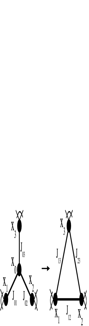
Figure 1: “Star-triangle” relation to reduce a three-connected spin $x_{0}$. The new bonds on the right are obtained in Eq. (II.1).

Rule VI: A spin $i$ (of any connectivity) for which the absolute weight $|J_{i,j^{\prime}}|$ of one bond to a spin $j^{\prime}$ is larger than the absolute sum of all its other bond-weights to neighboring spins $j\not=j^{\prime}$, i. e.

$$|J_{i,j^{\prime}}|>\sum_{j\not=j^{\prime}}|J_{i,j}|,$$ (6)

bond $J_{i,j^{\prime}}$ must be satisfied in any ground state. Then, spin $i$ is determined in the ground state by spin $j^{\prime}$ and it as well as the bond $J_{i,j^{\prime}}$ can be eliminated accordingly, as depicted in Fig. 2. Here, we obtain $H_{0}:=H_{0}-|J_{i,j^{\prime}}|$. All other bonds connected to $i$ are simply reconnected with $j^{\prime}$, but with reversed sign, if $J_{i,j^{\prime}}<0$.

This procedure is costly, and hence best applied after the other rules are exhausted. But it can be highly effective for very widely distributed bonds. In particular, since neighboring spins may reduce in connectivity and become susceptible to the previous rules again, further reductions may ensue, see Fig. 2.

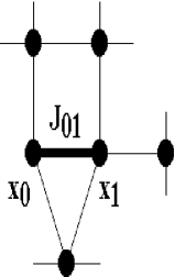
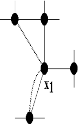
Figure 2: Illustration of Rule VI for “strong” bonds. Left, the local topology of a graph is shown for two spins, $x_{0}$ and $x_{1}$, connected by a bond $J_{0,1}$ (thick line). If $J_{0,1}>0$ (resp. $J_{0,1}<0$) satisfies Eq. (6), $x_{0}$ and $x_{1}$ must align (resp. anti-align) in the ground state and $x_{0}$ can be removed. Right, the remainder graph is show after the removal. The other bonds emanating from $x_{0}$ (dashed lines) are now directly connected to $x_{1}$ (potentially with a sign change, if $J_{0,1}<0$). This procedure may lead to a double bond (Rule III), if $x_{1}$ was already connected to a neighbor of $x_{0}$ before.

The bounds in Eqs. (3-II.1) become exact when the remaining graph takes on its ground state. Reducing even higher-connected spins would lead to new (hyper-)bonds between more than two spins, unlike Eq. (1). While such a reduction is possible and would eventually result in the complete evaluation of any lattice ground state, it would lead along the way to an exponential proliferation in the number of (hyper-)bonds in the system. This fact is a reflection of the combinatorial complexity of the glassy state, which will be explored in Ref. BoDu .

After a recursive application of these rules, the original lattice graph is either completely reduced (which is almost always the case below or near $p_{c}$), in which case $H_{o}$ provides the exact ground state energy already, or we are left with a highly reduced, compact graph in which no spin has less than four connections. We obtain the ground state of the reduced graph with an exact matching algorithm as used in Ref. HY , which together with $H_{o}$ provides the ground-state energy of the original diluted lattice instance.

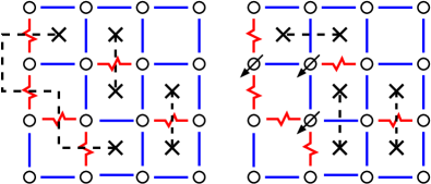
Figure 3: 2d spin glass with all spins up (left, up spins not shown). Straight lines are ferromagnetic, jagged lines are anti-ferromagnetic bonds. The dotted lines connect frustrated plaquettes (crosses). The bonds crossed by the dotted lines are unsatisfied. In the right part the ground state with three spins pointing down (all other up) is shown, corresponding to a minimum number of unsatisfied bonds.

II.2 Matching

Let us now explain just the basic idea of the matching algorithm, for the details, see Refs. bieche1980 ; SG-barahona82b ; derigs1991 . The method works for spin glasses which are planar graphs; this is the reason, why we apply periodic boundary conditions only in one direction. In the left part of Fig. 3 a small 2d system with open boundary conditions is shown. All spins are assumed to be “up”, hence all anti-ferromagnetic bonds are not satisfied. If one draws a dotted line perpendicular to all unsatisfied bonds, one ends up with the situation shown in the figure: all dotted lines start or end at frustrated plaquettes and each frustrated plaquette is connected to exactly one other frustrated plaquette. Each pair of plaquettes is then said to be matched. Now, one can consider the frustrated plaquettes as the vertices and all possible pairs of connections as the edges of a (dual) graph. The dotted lines are selected from the edges connecting the vertices and called a perfect matching, since all plaquettes are matched. One can assign weights to the edges in the dual graph, the weights are equal to the sum of the absolute values of the bonds crossed by the dotted lines. The weight $\Lambda$ of the matching is defined as the sum of the weights of the edges contained in the matching. As we have seen, $\Lambda$ measures the broken bonds, hence, the energy of the configuration is given by $E=-\sum_{\langle i,j\rangle}|J_{ij}|+2\Lambda$. Note that this holds for any configuration of the spins, since a corresponding matching always exists. Although Fig. 3 only shows a square lattice, a matching is always possible for any planar graph, such as the reduced, dilute lattices discussed here.

Obtaining a ground state means minimizing the total weight of the broken bonds (see right panel of Fig. 3), so one is looking for a minimum-weight perfect matching. This problem is solvable in polynomial time. The algorithms for minimum-weight perfect matchings MATCH-cook ; MATCH-korte2000 are among the most complicated algorithms for polynomial problems. Fortunately the LEDA library offers a very efficient implementation PRA-leda1999 , which we have applied here.

III Scaling Ansatz

Clearly, there exists a lowest bond fraction $p^{*}$, below which a glassy state is not possible. In particular, the lattice must exceed the bond-percolation threshold $p_{c}$ to exhibit any long-range correlated behavior and $p^{*}\geq p_{c}$ must hold. It is expected that $p^{*}=p_{c}$ for any continuous distribution, while for discrete distributions $p^{*}$ may be minutely larger than $p_{c}$ BF ; MKpaper ; Stiff1 . Accordingly, for two-dimensional bond-diluted lattices and a Gaussian bond distribution used here, we expect $p^{*}=p_{c}=1/2$ A+S . Similarly, it is expected that the correlation length near the critical point scales as

$$\xi(p)\sim(p-p^{*})^{-\nu^{*}}\quad\,$$ (7)

with $\nu^{*}=\nu=4/3$, well-known from 2-dimensional percolation.

The introduction of the bond density $p$ as new parameter permits a finite-size-scaling Ansatz in the limit $p\to p^{*}$. Combining the data for all $L$ and $p$ leads to a new variable $x=L/\xi(p)$, which has the chance of exhibiting scaling over a wider regime than for $L$ alone. As we have argued in Ref. BoCo , this Ansatz should take the form

$$\sigma(\Delta E)_{L,p}\sim\xi(p)^{y_{P}}~{}x^{y}~{}f(x),$$ (8)

as suggested by Refs. BBF ; BF . In principle, the Ansatz requires $L\gg 1$ and $\xi(p)\gg 1$. The scaling function $f$ was chosen as to approach a constant for $L\gg\xi(p)$.

Note that one basic assumption used here is that the exponent $y$ does not depend on the bond density $p$. Since a percolating cluster sufficiently above the percolation transition is effectively compact for large $L$, one may argue that asymptotic scaling properties of the spin glass should be uneffected by $p$. Reproducing the scaling of the undiluted lattice with the Ansatz in Eq. (8) with some accuracy would add support to this argument.

To obtain the exponent $y_{P}$ in Eq. (8) directly, one considers the limit $L\sim\xi(p)\to\infty$, i. e. $x\sim 1$. Then, one can show that at $p=p_{c}$ BBF ; BoCo

$$\sigma(\Delta E)_{L,p_{c}}\sim L^{y_{P}}.$$ (9)

We observe that due to the fractal nature of the percolating cluster at $p^{*}=p_{c}$, no long-range order can be sustained and defects possess a vanishing interface. Thus, $y_{P}\leq 0$ and the defect energy vanishes. In contrast, $y_{P}=0$ for discrete bond distributions such as $\pm J$, because $p^{*}>p_{c}$ and the interface energy $\sigma(\Delta E)_{L,p^{*}}$ becomes $L$-independent. As it turns out, with $y_{P}=0$ the scaling collapse greatly simplifies for $\pm J$ bonds, leaving continuous bonds with one extra exponent to account for. Hence, using Gaussian bonds, the accuracy obtained for the desired stiffness exponent $y$ diminishes, as the study in Ref. BoCo shows.

In case of a finite-temperature glass transition with divergent energy scales ($y>0$), universality provides us with the choice of the more convenient distribution, $\pm J$, to compute the stiffness exponent Stiff1 ; Stiff2 . Apparently, this universality brakes down below the lower critical dimension, $d<d_{l}\approx 2.5$ AMMP ; lowd , and a nontrivial value for $y$ is only obtained for continuous bonds HY . Thus, we have to take the exponent $y_{P}$ in Eq. (8) into account.

A scaling collapse is further complicated by the fact that the asymptotic regime of interest for the determination of $y$, namely $x\gg 1$ or $L\gg\xi(p)$, is hard to access for $p\to p^{*}$. Most data that reaches asymptotic scaling, i. e. $x\gg 1$, is typically obtained instead at intermediate values of $p$, sufficiently above $p^{*}$ to reach system sizes with $L\gg\xi(p)$ but small enough to exploit the reduction rules from Sec. II.1. As the analysis in Ref. BoCo suggest, in that regime the correlation length Eq. (7) may be too small to justify Eq. (8). Furthermore, it is clear that Eq. (7) is valid only close to $p_{c}$, leading possibly to wrong estimations for critical exponents obtained from finite-size scaling carter2003 . Also the finite-size corrections for the correlation length itself play probably an important role, which can bee seen from previous studies eschenbach1981 of two-dimensional percolation, where a significant change of the effective exponent $\nu$ was observed when changing the system size from $L=2$ to $L=10000$. Similarly, unknown scaling corrections missing in the form of Eq. (8) are likely to arise. Yet, experience shows that a focus on data with $L\gg\xi(p)$ for any $\xi(p)$ at least provides a satisfactory collapse in the $x\gg 1$ regime with an accurate prediction for the stiffness exponent $y$. There, unlike $y$, the exponents $\nu^{*}$ and $y_{P}$, and the scaling function $f(x)$, which are more closely associate with the scaling window near $p^{*}$, will not be accurately represented. In any fit of the data, their values are likely distorted to absorb the effect of unknown scaling corrections.

For our data analysis, we will therefore apply cuts to eliminate data outside of $x\gg 1$, and fit the remaining data to the form

$$\frac{\sigma(\Delta E)_{L,p}}{\xi(p)^{y_{P}}}\sim\left[\frac{L}{\xi(p)}\right]^{y}~{}f(\infty),$$ (10)

fixing $\xi(p)=(p-p^{*})^{-\nu^{*}}$, with $f(\infty)$, $p^{*}$, $\nu^{*}$, $y_{P}$, and $y$ as fitting parameters. Note that in this limit, $\nu^{*}$ and $y_{P}$ are not independent. Hence, we choose to fix $\nu^{*}=\nu=4/3$.

IV Numerical Experiments

In our numerical simulation, we have generated a large number of instances of symmetric Gaussian bond disorder on square lattices with open boundaries vertically, and periodic boundary conditions horizontally, as described in Ref. HY . But these instances are bond-diluted with a bond fraction of $p\geq p^{*}=p_{c}=1/2$. On this bond-diluted spin glass, the reduction algorithm from Sec. II.1 is applied to recursively remove as many spin variables as possible while exactly accounting for their contribution to the ground-state energy. Since the original lattice was a planar graph, the reduction method preserves this property for the remainder graph. Hence, the matching algorithm discussed in Sec. II.2 can be applied to the remainder graphs here to determine their exact ground states in polynomial time. In this manner, we study the defect energy $\sigma(\Delta E)$ both as a function of size $L$ and bond density $p$. We consider systems of sizes from maximally $L=150$ at $p=1$ to up to maximally $L=1000$ at $p=0.52$. At each pair of $L$ and $p$ we average typically well over about $10^{4}$ instances.

Figure 4: Logarithmic plot of $\sigma_{L}$ at $p=p^{*}=1/2$. An asymptotic power-law regime corresponding to Eq. (9), different from those for $p>p^{*}$, is reached quickly, and an asymptotic fit extrapolates to $y_{P}=-0.98(2)$.

Before we proceed to collapsing the data, it is instructive first to determine the exponent $y_{P}$ directly according to Eq. (9). Clearly, at $p=p^{*}$, diluted lattices are almost all entirely reducible with the rules given in Sec. II.1, and rarely is any subsequent optimization necessary. Hence, $L$ is limited only by the cost of reduction itself, memory space, and statistics. The data for the defect energy at $p^{*}=1/2$ is plotted in Fig. 4. The asymptotic fit yields about $y_{P}=-0.98(2)$. This value seems to suggest that $y_{P}=-1$, which would imply that the spin glass on a percolating cluster in two dimensions is essentially one-dimensional (where $y=-1$). Concluding that $y_{P}=-1$ is exact may be misguided: Ref. BBF obtained $y_{P}\approx-0.99$ on the basis of a scaling argument involving the numerical solution of an integral.

Figure 5: Plot on a logarithmic scale of the stiffness $\sigma$ as a function of system size $L$. The data is grouped into sets (connected by lines) parameterized by the bond density $p$. Most sets show a distinct scaling regime as indicated by Eq. (2) for sufficiently large $L$. In particular, the data for $p=0.51$ appears to never reach scaling and will be disregarded entirely.

To obtain an optimal scaling collapse of the data in accordance with the discussion in Sec. III, we focus on the data in the asymptotic scaling regime for each set. To this end, we chose for each data set a lower cut in $L$ by inspection of the data in Fig. 5. All data points below the cut for each $p$ are discarded, all data above are kept. Then the remaining data for all $L$ and $p$ are fitted to the four-parameter scaling form in Eq. (10). The resulting collapse is displayed in Fig. 6.

Initiating all of the parameters at near-optimal values, a least-square fit incorporating all the data shown in the collapse converges. The fitted values are $y=-0.281(3)$, $y_{P}=-0.77(5)$, $p^{*}=0.514(5)$, and $f(\infty)\approx 3.3$. Errors in this fit are estimates based the sensitivity on varying each parameter and have to be judged cautiously. It should be noted how essential the inclusion of the parameter $y_{P}$ was for the collapse, even obtaining a fitted value not too far from its actual value determined in Fig. 4. The discrepancy between the fitted value $y_{P}=-0.77$ and the accurate value $y_{P}=-0.99$ is due to the unknown scaling for $\xi(p)$ away from $p_{c}$ and the scaling-corrections for the approach Eq. (8), as discussed above.

Figure 6: Scaling plot of the data from Fig. 5 for $\sigma$, fitted to Eq. (10) as a function of the scaling variable $x=L/\xi(p)$ where $\xi(p)=(p-p^{*})^{-\nu^{*}}$. Data below the scaling regime in each set (i. e. below a certain value of $L$ for each $p$) from Figs. 5 was cut. The continuous line represent the power-law $[L/\xi(p)]^{-0.281}$, using the fitted value for $y$.

V Conclusion

We have used a scaling Ansatz proposed in Refs. BBF ; BF in conjunction with the spin reduction scheme of Refs. Stiff1 ; Stiff2 ; BoCo and exact ground-state calculations to study the defect energy at $T=0$ for bond-diluted lattices in two dimensions. The results for the stiffness exponent $y$ scale over 2 decades and are consistent with previous studies, validating the basic Ansatz. Yet, the obtained value $y=-0.281(3)$ is only of comparable accuracy to those studies, and the data collapse provides less of an advance than bond-diluted lattices did for higher-dimensional lattices. For one, in two dimensions there is no finite-temperature glass transition ($y<0$) and conventional studies at full connectivity are successful at reaching large lattice sizes already, avoiding the additional uncertainties of a multi-parameter fit. In this scenario, Ref. BoCo argued that such a collapse of data may provide diminishing returns for the computational effort. Similarly, it was observed there that a continuous bond distribution, considering the smaller size of elementary excitations under bond-reversal, leads to larger scaling corrections in $L$. Those scaling corrections are enhanced further by open boundaries, which have been observed previously to result in only weakly decreasing corrections HY ; Middle ; HM .

Our results indicate the validity of the recently proposed reduction scheme to determine the stiffness exponent $y$. Note that the fact that reduction works well in two-dimensions, where $T_{c}=0$ holds, does not imply definitely that it should work for $d>2$. Nevertheless, since the overall behavior in $d=2$ and higher dimensions is similar, it is highly probable that the reduction scheme is applicable also for higher dimensions Stiff1 ; Stiff2 , where no exact ground-state algorithms are available.

References

- (1) K. Binder and A. P. Young, Rev. Mod. Phys. 58, 801 (1986);
- (2) M. Mezard, G. Parisi, M. A. Virasoro, Spin glass theory and beyond, (World Scientific, Singapore 1987);
- (3) K. H. Fischer and J. A. Hertz, Spin Glasses (Cambridge University Press, Cambridge, 1991).
- (4) A. P. Young (ed.), Spin glasses and random fields, (World Scientific, Singapore 1998).
- (5) H. Rieger, L. Santen, U. Blasum, M. Diehl, and M. Jünger, J. Phys. A 29, 3939 (1996).
- (6) N. Kawashima and H. Rieger, Europhys. Lett. 39, 85 (1997).
- (7) A. K. Hartmann and A. P. Young, Phys. Rev. B 64, 180404(R) (2001).
- (8) J. Houdayer Eur. Phys. J. B 22, 479 (2001).
- (9) C. Amoruso, E. Marinari, O. C. Martin, and A. Pagnani, Phys. Rev. Lett. 91, 087201 (2003).
- (10) N. Kawashima and A. P. Young, Phys. Rev. B 53, R484 (1996).
- (11) E. Marinari, G. Parisi and J.J. Ruiz-Lorenzo, in: A.P. Young (ed.), Spin Glasses and Random Fields, (World Scientific, Singapore 1998).
- (12) A. K. Hartmann, Phys. Rev. E 59, 84 (1999).
- (13) A. C. Carter, A. J. Bray, and M. A. Moore, Phys. Rev. Lett. 88, 077201 (2002).
- (14) D. S. Fisher and D. A. Huse, Phys. Rev. Lett. 56, 1601 (1986).
- (15) A. J. Bray and M. A. Moore, Phys. Rev. Lett. 58, 57 (1987).
- (16) J.-P. Bouchaud, F. Krzakala, and O. C. Martin, Phys. Rev. B 68, 224404 (2003).
- (17) F. Krzakala and O.C. Martin, Phys. Rev. Lett. 85, 3013 (2000).
- (18) M. Palassini and A.P. Young, Phys. Rev. Lett. 85, 3017 (2000).
- (19) M. Palassini and A. P. Young, Phys. Rev. Lett. 83, 5126-5129 (1999).
- (20) B. W. Southern and A. P. Young, J. Phys. C: Solid State Phys. 10, 2179 (1977).
- (21) S. Kirkpatrick, Phys. Rev. B 15, 1533 (1977).
- (22) J. R. Banavar and M. Cieplak, Phys. Rev. Lett. 48, 832 (1982).
- (23) A. J. Bray and M. A. Moore, J. Phys. C: Solid State Phys. 17, L463 (1984).
- (24) M. Cieplak and J. R. Banavar, J. Phys. A: Math. Gen. 23, 4385 (1990).
- (25) S. Boettcher, Euro. Phys. J. B 33, 439 (2003).
- (26) A. K. Hartmann, Phys. Rev. E 60, 5135 (1999).
- (27) K. Hukushima, Phys. Rev. E 60, 3606 (2000)
- (28) A. K. Hartmann, A. J. Bray, A. C. Carter, M. A. Moore, and A. P. Young, Phys. Rev. B 66, 224401 (2002).
- (29) S. Boettcher, Euro. Phys. J. B 38, 83 (2004).
- (30) S. Boettcher, Europhys. Lett. 67, 453 (2004).
- (31) S. Boettcher and S. E. Cooke, Obtaining Stiffness Exponents from Bond-diluted Lattice Spin Glasses, cond-mat/0501547.
- (32) A. J. Bray and S. Feng, Phys. Rev. B 36, 8456 (1987).
- (33) I. Bieche, R. Maynard, R. Rammal, and J.P. Uhry, J. Phys. A 13, 2553 (1980).
- (34) F. Barahona, R. Maynard, R. Rammal, and J.P. Uhry, J. Phys. A 15, 673 (1982).
- (35) U. Derigs and A. Metz, Math. Prog. 50, 113 (1991).
- (36) F. Barahona, J. Phys. A: Math. Gen. 15, 3241 (1982).
- (37) M. R. Garey and D. S. Johnson, Computers and intractability (Freeman, San Francisco, 1979)
- (38) A.K. Hartmann and H. Rieger, Optimization Algorithms in Physics, (Wiley-VCH, Berlin, 2001)
- (39) A.K. Hartmann and H. Rieger, New Optimization Algorithms in Physics, (Wiley-VCH, Berlin, 2004)
- (40) S. Boettcher and P. Duxbury, in preparation.
- (41) W.J. Cook, W.H. Cunningham, W.R. Pulleyblank, and A. Schrijver, Combinatorial Optimization, (John Wiley & Sons, New York 1998).
- (42) B. Korte and J. Vygen, Combinatorial Optimization - Theory and Algorithms, (Springer, Heidelberg 2000).
-
(43)
K. Mehlhorn and St. Näher, The LEDA
Platform of Combinatorial and Geometric Computing (Cambridge
University Press, Cambridge 1999);
see also http://www.algorithmic-solutions.de - (44) Introduction to Percolation Theory, 2nd ed., D. Stauffer and A. Aharony, (Taylor and Francis, London, 1994).
- (45) J. R. Banavar, A. J. Bray, and S. Feng, Phys. Rev. Lett. 58, 1463 (1987).
- (46) S. Boettcher, in preparation.
- (47) A.C. Carter, A.J. Bray and M.A. Moore, J. Phys. A 36, 5699 (2003)
- (48) P.D. Eschbach, D. Stauffer, and H.J. Herrmann, Phys. Rev. B 23, 422 (1981)
- (49) A.A. Middleton, Phys. Rev. B 63, 060202(R) (2001).
- (50) A.K. Hartmann and M.A. Moore, Phys. Rev. Lett. 90, 127201 (2003).