Spin Hall effect of conserved current: Conditions for a nonzero spin Hall current

Abstract

We study the spin Hall effect taking into account the impurity scattering effect as general as possible with the focus on the definition of the spin current. The conserved bulk spin current (Shi et al. [Phys. Rev. Lett. 96, 076604 (2006)] ) satisfying the continuity equation of spin is considered in addition to the conventional one defined by the symmetric product of the spin and velocity operators. Conditions for non-zero spin Hall current are clarified. In particular, it is found that (i) the spin Hall current is non-zero in the Rashba model with a finite-range impurity potential, and (ii) the spin Hall current vanishes in the cubic Rashba model with a $\delta$-function impurity potential.

Spintronics is one of the most promising new technologies, where the spin degrees of freedom of electrons in semiconductors are manipulated and utilized for functions such as memory, operation, and communication. review ; Ohno One of the key routes to spintronics is to invent an efficient method to inject spins into semiconductors. In this respect, the intrinsic spin Hall effect (SHE) has attracted recent intensive attention since its theoretical proposal. Murakamiscience ; Sinovaprl This can give a larger effect by orders of magnitude than the extrinsic one based on the impurity scatterings proposed long before. Dyakonov ; Hirsch ; Zhang

Recently two experiments have been reported on observations of the SHE in GaAs and related materials.Kato ; Wunderlich Kato et al.Kato observed the Kerr rotation due to the spin accumulation ($\sim 10\mu_{B}(\mu\mathrm{m})^{-3}$) near the edges of the n-type GaAs sample. They suggested the extrinsic mechanism of the SHE since it was almost insensitive to the crystal orientation. Wunderlich et al.Wunderlich observed the circularly polarized LED signal from spin-polarized interfacial two-dimensional holes in p-type GaAs system. From an estimation of transport lifetime, they concluded that the spin accumulation is due to the intrinsic SHE.

The debates on the impurity effect on the intrinsic SHE have continued, which are in parallel to those for the anomalous Hall effect in ferromagnets. In the latter case, the intrinsic mechanism of Karplus-Luttinger KarplusLuttinger was criticized and extrinsic mechanisms due to impurity scatterings were proposed. Smit The Hall conductivity is a singular function as the disorder strength approaches zero. In the metallic case, the vertex correction in the diagrammatic language incorporates a deviation of the electronic distribution function from equilibrium, and it represents the dissipative current. This situation is similar also in the spin Hall current.

Actually, the disorder effect on the spin Hall current of the Rashba model in two dimensions has been intensively studied. Sinova et al. Sinovaprl obtained the universal value $e/(8\pi)$ note8pi for the spin Hall conductivity (SHC) $\sigma_{H}^{s}$ without disorder. When the self-energy correction due to impurity scattering is taken into account, the SHC $\sigma_{H}^{s}$ is reduced continuously as a function of the disorder strength from the universal value $e/(8\pi)$. Loss On the other hand, Inoue et al. Inoue studied the vertex correction and found that $\sigma^{s}_{H}$ vanishes in the clean limit within the Born approximation. Furthermore, it has been shown that the SHC $\sigma^{s}_{H}$ vanishes for any value of the lifetime $\tau$ using the Keldysh formalism, Halperin ; Liu ; Liu2 the Kubo formula analytically, Dimitrova ; Chalaev ; Raimondi and numerically, Sheng ; Nomura2 and the Boltzmann equation. Khaetskii Thus after long debates, people have reached the consensus that the SHC $\sigma^{s}_{H}$ for the Rashba model vanishes for any $\tau$. previous

However, the vanishing result of $\sigma^{s}_{H}$ depends on the definition of the spin current. In the previous calculations on the SHC, the spin current is defined ad hoc as a symmetrized product of the spin and the velocity $J_{s}=\frac{1}{2}\{v_{y},s_{z}\}$, where $v_{y}=\partial H/\partial p_{y}$, in response to the electric field $\mathbf{E}$ along the $x$ axis. However, this “conventional” definition of spin current loses its physical foundation when the spin-orbit coupling is present and the conservation law of the spin is violated. This is an important issue since the concept of “current” depends crucially on conservation; non-local effects of the current comes from the fact that an incoming flow goes out without loss. Therefore we need to search for a proper definition of a conserved spin current in the bulk. From this viewpoint, the conserved spin current ${\cal{\bm{J}}}_{s}$ PZhang deserves scrutiny. If $\int dV\langle\dot{s}_{z}\rangle=0$, it satisfies the Onsager’s reciprocity relation and the continuity equation for the spin in the bulk: $\partial_{t}\langle s_{z}\rangle+\nabla\cdot{\vec{\cal J}}_{s}=0$. Furthermore it is free from an artifact that the spin current is proportional to time derivative of the spin operator; Dimitrova ; Chalaev hence, the spin Hall current can be nonzero even for the Rashba model. Even though the experiments on the SHE up to now Kato ; Wunderlich detect the spin accumulation at the sample edges, we stick here to the SHE defined by the bulk spin current. This is because we consider that the generation of the conserved spin current in the bulk is a more fundamental phenomenon than the spin accumulation at edges, which is not solely determined by this spin current since the continuity equation for the spin is not satisfied there. In principle, there should be other means to detect the SHE without using the spin accumulation such as voltage measurement with the injected spin current. spininjection

In this paper, we study the SHE as generally as possible taking into account the disorder with the definitions of the conventional and conserved spin current. Applying this consideration, some new results are obtained for the Rashba and cubic Rashba models. We employ the Keldysh formalism, Rammer ; Halperin ; mahan by which the infinite series of the Feynman diagrams both for the self-energy and vertex correction are taken into account compactly, and the expression for the SHC is obtained for both definitions of the spin current described above.

We consider a generic model with spin-orbit coupling with a random impurity potential, this random potential is assumed to be spin-independent, and the time-reversal symmetric model exclusively. In the Keldysh formalism, a Green’s function matrix $\underline{G}$ is introduced,

$$\underline{G}=\left(\begin{array}[]{cc}G^{R}&G^{<}\\ 0&G^{A}\end{array}\right),$$ (1)

where the superscripts $R$, $A$, and $<$ denote the retarded, advanced and lesser Green’s functions, respectively. The self-energy matrix $\underline{\Sigma}$ is defined similarly. The Green’s functions satisfy

$$(G^{R})^{-1}\otimes G^{<}-G^{<}\otimes(G^{A})^{-1} = \Sigma^{<}\otimes G^{A}-G^{R}\otimes\Sigma^{<},$$

$$({\cal G}_{0}^{-1}-\Sigma^{R,A})\otimes G^{R,A} = \delta(1-2),$$ (3)

where $(A\otimes B)(1,2)\equiv\int d3A(1,3)B(3,2)$ and ${\cal G}_{0}$ is the unperturbed Green’s function. We then separate the center-of-mass and the relative coordinates and perform the Fourier transform to the relative coordinates. mahan ; Rammer The final result is written in terms of the center-of-mass coordinates $(T,\mathbf{R})$ and the relative momentum $(\omega,\mathbf{p})$. We put the constant electric field $\mathbf{E}=(E,0,0)$ and look for solutions independent of $T$ and $\mathbf{R}$. Therefor the quantum Boltzmann equation (QBE) is written by

$$[{\underline{G}},~{}H]=-ie{\mathbf{E}}\cdot{\mathbf{\nabla_{p}}}{\underline{G}}-\frac{i}{2}e{\mathbf{E}}\cdot\left\{{\mathbf{\nabla}_{p}}H,~{}\partial_{\omega}{\underline{G}}\right\}$$

$$-\frac{i}{2}e{\mathbf{E}}\cdot\left(\left\{{\mathbf{\nabla}_{p}}{\underline{\Sigma}},~{}\partial_{\omega}{\underline{G}}\right\}-\left\{\partial_{\omega}{\underline{\Sigma}},~{}{\mathbf{\nabla}_{p}}{\underline{G}}\right\}\right)+[{\underline{\Sigma}},~{}{\underline{G}}].$$ (4)

Here one can show from Eq. (4) that the time derivative $\dot{{\cal O}}$ of an arbitrary operator ${\cal O}$, which is independent of $\mathbf{p}$, $\mathbf{R}$, $T$ and $\omega$, has a vanishing expectation value in the steady state, $\langle\dot{{\cal O}}\rangle=0$, even with a general form of the impurity potential. Dimitrova ; Chalaev We start with

$$\langle\dot{{\cal O}}\rangle=\frac{1}{i}\int\frac{d\omega}{2\pi}\int\frac{d^{2}p}{(2\pi)^{2}}\mathrm{tr}(\dot{{\cal O}}G^{<})$$

$$\ \ \ =\int\frac{d\omega}{2\pi}\int\frac{d^{2}p}{(2\pi)^{2}}\mathrm{tr}({\cal O}[{\underline{G}},H]^{<}),$$ (5)

where $[\ \ ]^{<}$ denotes the lesser (upper right) component of the matrix in the Keldysh space. Eq. (4) is plugged into Eq. (5), and evaluate the respective terms in the RHS of Eq. (4). The first term $ie\mathbf{E}\cdot{\mathbf{\nabla}_{p}}G^{<}$ becomes zero after an integration over $\mathbf{p}$. The second term vanishes after an $\omega$-integration. The third and fourth terms vanish after partial integrations in terms of $\mathbf{p}$ and $\mathbf{\omega}$. Lastly, to evaluate the last term $([\underline{\Sigma},\ \underline{G}]^{<})$, we need a relationship between the self-energies and Green’s functions. We employ the self-consistent Born approximation [the diagrams in Fig. 1 (a) and (b)] Crepieux for the impurity scattering. Up to the second order it is given by

$$\underline{\Sigma}(\omega,\mathbf{p})=n_{i}\int\frac{d^{2}p^{\prime}}{(2\pi)^{2}}\left|V_{\mathbf{p},\mathbf{p}^{\prime}}\right|^{2}\underline{G}(\omega,\mathbf{p}^{\prime})$$

$$+n_{i}\int\frac{d^{2}p^{\prime}\,d^{2}p^{\prime\prime}}{(2\pi)^{4}}V_{\mathbf{p},\mathbf{p}^{\prime}}V_{\mathbf{p}^{\prime},\mathbf{p}^{\prime\prime}}V_{\mathbf{p}^{\prime\prime},\mathbf{p}}\underline{G}(\omega,\mathbf{p}^{\prime})\underline{G}(\omega,\mathbf{p}^{\prime\prime}).\ \ \$$ (6)

where $n_{i}$ is an impurity density, and $V_{\mathbf{p},\mathbf{p}^{\prime}}$ is the Fourier transform of the impurity potential. From the second Born approximation Eq. (6) one can easily show $\langle\dot{\cal O}\rangle=0$ for arbitrary forms of impurity potentialsNote . This holds true even for higher-order Born approximation. On the other hand, for the charge current $\mathbf{v}=\dot{\mathbf{R}}$, this argument does not apply, and $\langle\mathbf{v}\rangle$ can be nonzero in the steady state as expected.

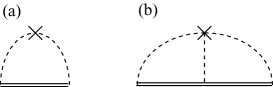
Figure 1: Diagrammatic representation of the self-energy $\underline{\Sigma}$ in the present self-consistent approximation. Doubled line is the dressed Keldysh Green’s function $\underline{G}$. Dashed line with a cross denotes the average over the impurity positions in the second order for (a) and in the third order (b), respectively.

Now we proceed to a closed form of the SHC. The expectation value of the conventional spin current $J_{s}\equiv\frac{1}{2}\{v_{y},s_{z}\}$ is obtained as

$$\frac{\langle J_{s}\rangle}{E} = -\lim_{E\rightarrow 0}\frac{i}{2E}\int\frac{d\omega}{2\pi}\frac{d^{2}p}{(2\pi)^{2}}\mathrm{tr}\left[s_{z}\left\{\frac{\partial H}{\partial p_{y}},\underline{G}\right\}\right]_{E}^{<},$$ (7)

where $[\ ]_{E}$ implies that we retain the terms linear in a uniform electric field $\mathbf{E}=E\hat{x}$.

Let us turn to the second definition of the spin current ${\vec{\cal J}}_{s}$ as proposed by Shi et al. PZhang ${\vec{\cal J}}_{s}$ is defined to satisfy $\partial_{t}\langle s_{z}\rangle+\nabla\cdot{\vec{\cal J}}_{s}=0$, and is divided into $\langle{\vec{J}}_{s}\rangle+{\vec{P}}_{\tau}$, where ${\vec{J}}_{s}=\frac{1}{2}\{{\vec{v}},s_{z}\}$. The second term ${\vec{P}}_{\tau}$ is called the torque dipole density, and is required to satisfy $\lim_{\Omega\rightarrow 0}\lim_{{\vec{Q}}\rightarrow 0}(\langle\dot{s}_{z}(\Omega,\vec{Q})\rangle+i\vec{Q}\cdot\vec{P}_{\tau}(\Omega,{\vec{Q}}))=0$, where ($\Omega,{\vec{Q}}$) are the Fourier components of the center-of-mass coordinates. We put $Q_{x}=0$, and take the limit $Q_{y}=Q\rightarrow 0$, i.e., ${P}_{\tau}\equiv{\vec{P}}_{\tau}\cdot\hat{\mathbf{y}}=-\lim_{\Omega\rightarrow 0}\lim_{Q\rightarrow 0}\frac{1}{iQ}\langle\dot{s}_{z}(\Omega,Q)\rangle$. More explicitly, $\mathbf{E}$ is spatially modulated along the y-axis, $\mathbf{E}=Ee^{iQY-i\Omega T}\hat{\mathbf{x}}$. PZhang Note that $\langle\dot{s}_{z}(0,0)\rangle=0$ from Eq. (5), which means $P_{\tau}$ is finite and well-defined. In response to the electric field, the Green’s function $\underline{G}$ and the self-energy $\underline{\Sigma}$ acquire terms proportional to $e^{iQY-i\Omega T}$. $P_{\tau}$ is expressed as

$$P_{\tau}=-i\lim_{Q\rightarrow 0}\frac{1}{Q}\int\frac{d\omega}{2\pi}\int\frac{d^{2}p}{(2\pi)^{2}}\mathrm{tr}(s_{z}[H,\underline{G}]^{<}).$$ (8)

We first write down the QBE to the linear order in $E$ and to the linear order in $\Omega$ or $Q$. Next, we replace the term $[H,\underline{G}]^{<}$ in Eq. (8) with the corresponding term in the QBE. While there arise a number of terms, most of them give no contribution to $P_{\tau}$ after partial integrations over $p_{i}$ or $\omega$. To calculate the remaining terms, we note that this electric field necessarily accompanies a magnetic field according to the Maxwell equation. To deal with the response to these two fields, it is convenient to consider the corresponding vector potential, $\mathbf{A}=(Ae^{iQY-i\Omega T},0,0)$. Relevant terms in the QBE are classified to those proportional to $i\Omega A=E$ (electric field) or those proportional to $-iQA=B$ (magnetic field). The resulting form is a sum of the contributions from the response to a dc electric field $E\hat{x}$ and that to a dc magnetic field $B\hat{z}$:

$$\frac{{\cal J}_{s}}{E}=\lim_{E\rightarrow 0}\frac{i}{E}\int\frac{d\omega}{2\pi}\frac{d^{2}p}{(2\pi)^{2}}\mathrm{tr}\left[\frac{1}{2}s_{z}\left\{\frac{\partial\underline{\Sigma}}{\partial p_{y}},\ \underline{G}\right\}\right]^{<}_{E}$$

$$+\lim_{B\rightarrow 0}\frac{i}{B}\int\frac{d\omega}{2\pi}\frac{d^{2}p}{(2\pi)^{2}}\mathrm{tr}\left[s_{z}\underline{G}\!-\frac{1}{2}s_{z}\left\{\frac{\partial\underline{\Sigma}}{\partial\omega},\,\underline{G}\right\}\right]^{<}_{B}.$$ (9)

Here ${\cal J}_{s}={\vec{\cal J}}_{s}\cdot\hat{\mathbf{y}}$, and $[\ ]_{B}$ retains the terms linear in an uniform magnetic field $\mathbf{B}=B\hat{\mathbf{z}}$. Because $\mathbf{B}$ does not drive the system off-equilibrium, the relation in equilibrium, $G^{<}_{0}=(1-\tanh(\omega/{2k_{B}T}))(G^{A}_{0}-G^{R}_{0})/2$, is satisfied even in the presence of $\mathbf{B}=B\hat{\mathbf{z}}$. The details of the derivation of Eq. (9) will be presented elsewhere. Sugimotolong . Remarkably, in calculating the total conserved spin current ${\cal J}_{s}=\langle J_{s}\rangle+P_{\tau}$, there appears a term in $P_{\tau}$ which exactly cancels $\langle J_{s}\rangle$. We also note that this formula is quite generic and applies to any models. The expression of the charge current is obtained just by replacing $s_{z}$ by $-e$ in Eq. (9), and the $B$-term in the final formula is reminiscent of the Streda formula. Streda1 ; Streda2

We now discuss the explicit models based on the results obtained above. Here we condider the Rashba model

$$H=\frac{{\bf p}^{2}}{2m}+\lambda({\bm{\sigma}}\times\mathbf{p})\cdot{\hat{z}}+v,$$ (10)

and the cubic Rashba model

$$H=\frac{{\bf p}^{2}}{2m}+\frac{i\lambda}{2}(p_{-}^{3}\sigma_{+}-p_{+}^{3}\sigma_{-})+v.$$ (11)

Here, ${\bm{\sigma}}=(\sigma_{x},\sigma_{y},\sigma_{z})=2\mathbf{s}$ is the Pauli matrix, $p_{\pm}=p_{x}\pm ip_{y}$, $\sigma_{\pm}=\sigma_{x}\pm i\sigma_{y}$ and $v$ is an impurity random potential. We take the unit where $\hbar=c=1$. The Rashba model represents an n-type semiconductor in two-dimensional heterostructure. The second term in Eq. (10) represents the spin-orbit coupling with an inversion-symmetry-breaking potential along the $z$ direction perpendicular to the plane. As noticed in Refs. Dimitrova, and Chalaev, , $J_{s}$ is proportional to $\dot{s}_{y}$: $J_{s}=\frac{p_{y}\sigma_{z}}{2m}=\frac{[H,\sigma_{y}]}{4im\lambda}$. Therefore from the generic argument in Eq. (5), there occurs no spin Hall current when this definition of the spin current is employed for the Rashba model (Table I(a)). This result is consistent with previous works using various methods, including the calculations in the clean limit by Kubo formula, Inoue ; Raimondi and Keldysh formalism. Liu For finite $\tau$ $(\epsilon_{F}\tau\gg 1)$, it is also consistent with the analytic Dimitrova ; Chalaev and numerical Sheng ; Nomura2 results by Kubo formula, and with the results by Keldysh formalism. Halperin ; Liu2 The calculation in Ref. Chalaev by Kubo formula for finite $\tau$ $(\epsilon_{F}\tau\gg 1)$ is similar to ours by the Keldysh formalism. Nevertheless, our approach better reveals the reason why the spin Hall current generally vanishes when $J_{s}\propto{\dot{s}}_{y}$.

The cubic Rashba model, on the other hand, describes the heavy-hole bands of cubic semiconductors in heterostructute. The conventional spin current $J_{s}$ can no longer be expressed as $\dot{\cal O}$; hence the previous argument for vanishing spin Hall current does not apply. Indeed, the resulting SHC is nonzero BZn [Table I(b) ], which is consistent with Refs. holegas1, and holegas2, . Therefore the zero or nonzero spin Hall current for the conventional spin current $J_{s}$ is mostly determined whether it is expressed by the time derivative of some local operator or not.

Next we turn to the conserved spin current ${\cal J}_{s}$. Both in the Rashba and the cubic Rashba models, the $B$-term in Eq. (9) vanishes, because the Hamiltonian lacks a $\sigma_{z}$-term, and the self-energy is independent of the spin. The remaining $E$-term in Eq. (9) for the Rashba model is calculated as follows. In the first Born approximation [the first term in Eq. (6)], ${\cal J}_{s}=0$ for general $V_{\mathbf{p}-\mathbf{p}^{\prime}}$. In the second Born approximation, we obtain

$${\cal J}_{s}=-\frac{in_{i}}{4}\int\frac{d\omega}{2\pi}\frac{d^{2}p}{(2\pi)^{2}}\frac{d^{2}p^{\prime}}{(2\pi)^{2}}\frac{d^{2}p^{\prime\prime}}{(2\pi)^{2}}\mathrm{tr}\Big{[}\sigma_{z}\big{[}\underline{G}(\omega,\mathbf{p})$$

$$\ \ \cdot\underline{G}(\omega,\mathbf{p}^{\prime})\underline{G}(\omega,\mathbf{p}^{\prime\prime})\big{]}_{E}^{<}\frac{\partial(V_{\mathbf{p}-\mathbf{p}^{\prime}}V_{\mathbf{p}^{\prime}-\mathbf{p}^{\prime\prime}}V_{\mathbf{p}^{\prime\prime}-\mathbf{p}})}{\partial p^{\prime}_{y}}\Big{]}.$$ (12)

Even for higher-order Born approximation, the formula for ${\cal J}_{s}$ can be written down. We can then see that ${\cal J}_{s}$ always depends on $\partial_{p_{y}}V$, and the spin Hall current for ${\cal J}_{s}$ is extrinsic for both the Rashba and the cubic Rashba models, depending explicitly on the impurity potential. All these considerations are summarized in Table I. With the $\delta$-impurity potential the conserved spin Hall current vanish both for the Rashba model and the cubic Rashba model. We note that calculated the conserved SHC without disorder is $\sigma^{s}_{H}=e/8\pi$ for the Rashba model and $\sigma^{s}_{H}=-9e/8\pi$ in the cubic Rashba model. PZhang These results are reproduced in our calculations by neglecting the self-energy of the lesser Green’s function and taking the clean limit.

(a) Rashba model Impurity potential Born approx. Definition of spin current       $\langle J_{s}\rangle$ ${\cal{J}}_{s}$ $\delta(\mathbf{r})$ 1st/higher 0 IK 0 $V_{\mathbf{p}-\mathbf{p}^{\prime}}$ 1st 0 long 0 higher 0 Finite

(b) Cubic Rashba model

Impurity potential	Born approx.	Definition of spin current
		$\langle J_{s}\rangle$	${\cal J}_{s}$
$\delta(\mathbf{r})$	1st/higher	Finite holegas1 ; holegas2	0
$V_{\mathbf{p}-\mathbf{p}^{\prime}}$	1st	Finite	0
	higher	Finite	Finite

Table 1: Spin Hall effect in the (a) (linear) Rashba model and (b) cubic Rashba model, with various types of the impurity potential for the two different definitions: $\langle J_{s}\rangle$ is the conventional spin current, $J_{s}=\frac{1}{2}\{v_{y},s_{z}\}$, and ${\cal{J}}_{s}$ is the conserved effective spin current, ${\cal{J}}_{s}=\langle J_{s}\rangle+P_{\tau}$. We show the new results in the boldface.

We now demonstrate the finite spin Hall current for ${\cal{J}}_{s}$ in the Rashba model with the short-range (not $\delta$-function) impurity potential $V(r)=Ue^{-(\frac{r}{\beta})^{2}}$ with $\beta\Lambda\ll 1$, where $U$ is the magnitude of the impurity potential, $\beta$ is the size of the potential range and $\Lambda$ is a momentum cutoff. As an approximation, we substitute the Green’s functions in Eq. (9) with those for the $\delta$-function impurity potential, and calculate ${\cal J}_{s}$. Figure 2 shows the results for the SHC $\sigma^{s}_{H}$ in the parameter space of $\lambda p_{F}/\varepsilon_{F}$ and $\tau\varepsilon_{F}$. Since the SHC $\sigma^{s}_{H}$ is proportional to $(\beta p_{F})^{2}$ and $U/\epsilon_{F}$ within our calculation scheme, the vertical axis is set to be $\sigma^{s}_{H}(\beta p_{F})^{-2}(\epsilon_{F}/U)$, and is normalized by the universal value $e/(8\pi)$.

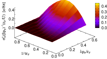
Figure 2: Contour map of the SHC $\sigma^{s}_{H}$. It has the maximum value nearly along $\alpha=2\lambda p_{F}\tau=1$. The momentum cutoff is set to be $\Lambda\approx 3p_{F}$, and $U/\varepsilon_{F}=0.02$.

$\sigma^{s}_{H}$ has a maximum value along the line $\alpha=2\lambda p_{F}\tau\cong 1$ at each $\lambda$ and the maximum value depends on $\log(\Lambda/p_{F})$. This conserved spin current is nonzero even for the Rashba model in two dimensions.

The above results give a hint to look for systems showing the spin Hall current. One important feature is that the Hamiltonian should involve $s_{z}$. Luttinger model Murakamiscience satisfies this condition while the cubic Rashba model does not. Therefore the complete confinement of the electronic motion along one direction is not desirable. We have assumed that the spin-orbit interaction is unchanged by disorder. In reality, the impurity potential $v(\mathbf{r})$ induces a spin-orbit coupling as $(\mathbf{p}\times\nabla v)\cdot\mathbf{s}$. This is also expected to contribute to the extrinsic spin Hall effect. Engel This effect is beyond the scope of the present paper.

In conclusion, we derived a general exact formula of the spin Hall conductivity for the two kinds of spin current: (a) the product of spin and velocity operators and (b) the effective conserved spin current. The conditions for the non-zero spin Hall current has been clarified and are applied to the Rashba and cubic Rashba models.

The authors thank H. Fukuyama, B. I. Halperin, M. Onoda, and S. Y. Liu for stimulating discussions. The work is supported by the Grants-in-aid for Scientific Research and NAREGI Nanoscience Project from the Ministry of Education, Culture, Sports, Science, and Technology.

References

- (1) S. A. Wolf, et al., Science 294, 1488 (2001).
- (2) H. Ohno, Science 281, 951 (1998).
- (3) S. Murakami, N. Nagaosa, and S. C. Zhang, Science 301, 1348 (2003).
- (4) J. Sinova et al., Phys. Rev. Lett. 92, 126603 (2004).
- (5) M. I. D’yakonov and V. I. Perel’, JETP Lett. 13, 467 (1971).
- (6) J. E. Hirsch, Phys. Rev. Lett. 83, 1834 (1999).
- (7) S. Zhang, Phys. Rev. Lett. 85, 393 (2000).
- (8) Y. K. Kato, et al., Science 306, 1910 (2004).
- (9) J. Wunderlich, B. Kaestner, J. Sinova, and T. Jungwirth, Phys. Rev. Lett. 94, 047204 (2005).
- (10) R. Karplus and J. M. Luttinger, Phys. Rev. 95, 1154 (1954).
- (11) J. Smit, Physica 21, 877 (1955); 24, 39 (1954).
- (12) We take the electron charge to be .
- (13) J. Schliemann and D. Loss, Phys. Rev. B 69, 165315 (2004).
- (14) J. I. Inoue, G. E. W. Bauer, and L. W. Molenkamp, Phys. Rev. B 70, 041303(R) (2004).
- (15) E. G. Mishchenko, A. V. Shytov, and B. I. Halperin, Phys. Rev. Lett. 93, 226602 (2004).
- (16) S. Y. Liu and X. L. Lei, cond-mat/0411629.
- (17) S. Y. Liu, X. L. Lei, and N. J. M. Horing, Phys. Rev. B 73, 035323 (2006).
- (18) O. V. Dimitrova, cond-mat/0405339.
- (19) O. Chalaev and D. Loss, Phys. Rev. B 71, 245318 (2005).
- (20) R. Raimondi and P. Schwab, Phys. Rev. B 71, 033311 (2005).
- (21) D. N. Sheng, L. Sheng, Z. Y. Weng, and F. D. M. Haldane, Phys. Rev. B 72, 153307 (2005).
- (22) K. Nomura, J. Sinova, N. A. Sinitsyn, and A. H. MacDonald, Phys. Rev. B72, 165316 (2005). This paper supersedes the previous one by the same authors (K. Nomura, J. Sinova, T. Jungwirth, Q. Niu, and A. H. MacDonald, Phys. Rev. B 71, 041304(R) (2005)).
- (23) A. Khaetskii, Phys. Rev. Lett. 96, 056602 (2006).
- (24) The previous version of the manuscript (cond-mat/0503475-v1) contained a serious error in convergence of the numerical solution to the integral equation for the self-energy. This led to a wrong conclusion for finite in the Rashba model with -function impurities.
- (25) J. Shi, P. Zhang, D. Xiao, and Q. Niu, Phys. Rev. Lett. 96, 076604 (2006).
- (26) A. Azevedo et, al., J. Appl. Phys. 97, 10C715 (2005).
- (27) J. Rammer and H. Smith, Rev. Mod. Phys. 58, 323 (1986).
- (28) G. D. Mahan, Many-Particle Physics (Plenum Press, New York, 1990) pp. 671-686.
- (29) A. Crépieux and P. Bruno, Phys. Rev. B 64, 014416 (2001).
- (30) This second Born diagram gives the skew-scattering contribution in the case of anomalous Hall effect Crepieux .
- (31) N. Sugimoto et, al., unpublished.
- (32) L. Smrčka and P. Středa, J. Phys. C: Solid State Phys. 10, 2153 (1977).
- (33) P. Středa and J. Phys. C: Solid State Phys, 15, L717 (1982).
- (34) B. A. Bernevig, S. C. Zhang, cond-mat/0412550.
- (35) B. A. Bernevig and S. C. Zhang, Phys. Rev. Lett. 95, 016801 (2005).
- (36) S. Y. Liu and X. L. Lei, Phys. Rev. B72, 155314 (2005).
- (37) This result is consistent with Refs. Inoue, ; Halperin, ; Liu, ; Liu2, ; Dimitrova, ; Chalaev, ; Raimondi, ; Sheng, ; Nomura2, ; Khaetskii, .
- (38) S. Y. Liu and X. L. Lei, cond-mat/0502392.
- (39) H. A. Engel, B. I. Halperin, and E. I. Rashba, Phys. Rev. Lett. 95, 166605 (2005).