Phase behavior of a nematic liquid crystal in contact with a chemically and geometrically structured substrate

Abstract

A nematic liquid crystal in contact with a grating surface possessing an alternating stripe pattern of locally homeotropic and planar anchoring is studied within the Frank–Oseen model. The combination of both chemical and geometrical surface pattern leads to rich phase diagrams, involving a homeotropic, a planar, and a tilted nematic texture. The effect of the groove depth and the anchoring strengths on the location and the order of phase transitions between different nematic textures is studied. A zenithally bistable nematic device is investigated by confining a nematic liquid crystal between the patterned grating surface and a flat substrate with strong homeotropic anchoring.

I Introduction

The contact of nematic liquid crystals (NLCs) with structured solid substrates offers the possibility to manipulate the orientation of the adjacent liquid crystal molecules in a controlled way. For example, substrates with topographic structures influence anchoring of liquid crystal molecules and induce elastic distortions and flexoelectric polarizations within a contacting NLC. Alignment of liquid crystal molecules can also be governed by the pattern of boundary lines between different regions on a flat substrate and the NLC elasticity. Adjacent regions of planar and homeotropic anchoring within a single substrate have been created, for example, by micro-contact printed polar and apolar thiols, respectively, on an obliquely evaporated ultra-thin gold layer. Whereas many experimental and theoretical studies have focussed on the understanding of the interactions and phase behavior of NLCs in contact with either geometrically structured substrates (see e.g., berr:72 ; faet:87 ; bari:96 ; moce:99 ; four:99 ; barb:99 ; brow:00 ; patr:02 ; chun:02 ; lu:03 ; parr:03 ; brow:04 ; parr:04 ) or chemically patterned substrates (see e.g., ong:85 ; barb:92 ; qian:96 ; qian:97 ; gupt:97 ; lee:01 ; kond:01 ; wild:02 ; wild:03 ; kond:03 ; park:03 ; zhan:03 ; tsui:04 ; yu:04 ; poni:04 ), NLCs near geometrically structured and chemically patterned substrates have not been investigated yet. In view of the rich behavior of NLCs even on geometrically structured or chemically patterned substrates, a combination of both surface treatments may open new possibilities for an improved performance of NLC cells. Here we study a NLC in contact with a grating surface possessing an alternating stripe pattern of locally homeotropic and planar anchoring within the Frank–Oseen model fran:58 ; dege:93 , whereby the anchoring energy function is given by the Rapini–Papoular expression rapi:69 . Taking into account both chemical and geometrical surface pattern is particularly interesting because of the possibility of bistable anchoring, which is important for low power consumption liquid crystal displays. In bistable nematic devices there are two stable nematic director orientations which have substantially different tilt angles. The zenithally bistable nematic devices that have been studied recently consist of a NLC confined between a grating surface and a flat surface parr:03 ; brow:04 ; parr:04 ; davi:02 . These surfaces are coated with a homeotropic agent. While such a device is characterized by both a high shock stability and a low power consumption, the deep grating structure leads to a reduction of the contrast of the display krie:02 . On the basis of our calculations we expect that an additional chemical surface pattern allows one to use rather a shallow grating surface instead of a deep one.

The structure of the paper is as follows. In Section II two models of a patterned grating surface are introduced and phase diagrams of a NLC in contact with the model surfaces are discussed. In particular we show how phase transitions between different nematic textures vary with the groove depth and the anchoring strengths. The phase behavior and director profile of a NLC confined between a patterned grating surface and a flat surface subject to strong homeotropic anchoring is investigated in Sec. III. Our results are summarized in Sec. IV.

II NLC in contact with a chemically and geometrically patterned substrate

We first consider a semi-infinite system consisting of a NLC in contact with a single, patterned grating surface. Two models of the surface grating are investigated. In model ${\mathcal{A}}$, a sinusoidal grating surface is assumed. This leads to the Euler–Lagrange equation for a two-dimensional director field, which is then solved numerically. In model ${\mathcal{B}}$, we choose a special form of the surface grating which, albeit not given explicitly by a simple formula, has the great advantage that the problem can be reformulated in terms of a semi-infinite system with a flat patterned substrate, and for the latter we have developed previously an efficient method of finding the equilibrium director field kond:01 .

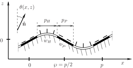
Figure 1: The system under consideration consists of a nematic liquid crystal (NLC) in contact with a grating surface with an alternating stripe pattern of locally homeotropic anchoring (white bars) and homogeneous planar anchoring (black bars). The stripes are orientated along the $y$ axis perpendicular to the plane of the figure. The projection of the widths of the stripes onto the $x$-axis and the anchoring strengths are designated as $p_{H}=p/4$, $p_{P}=p/4$ and $w_{H}$, $w_{P}$, respectively, and the midlines of the planar anchoring stripes are located at $x=np/2$ with $n=0,\pm 1,\pm 2,\cdots$; $\wp$ is the period of the chemical pattern which is half the period of the surface grating $p$. The tilt of the nematic director with respect to the $z$-axis is denoted by $\theta(x,z)$.

II.1 Model ${\mathcal{A}}$: Sinusoidal grating surface

Let us consider a NLC in contact with a single grating surface and assume that the surface profile $z_{0}(x)$ is given by

$$z_{0}(x)=A\sin\left(qx\right)\,,$$ (1)

where $A$ is the groove depth and $p=2\pi/q$ is the period. Such a surface structure can be fabricated, for instance, using an interferometric exposure technique (see Ref. brow:04 and references therein). As Figure 1 illustrates, the surface exhibits a pattern consisting of alternating stripes of locally homeotropic and homogeneous planar anchoring. The system is translationally invariant in the $y$ direction. We focus on shallow grooves for which the nematic director ${\bf\hat{n}}$ can be constrained to the plane perpendicular to the direction of the surface grooves. The orientation of ${\bf\hat{n}}$ is therefore given solely by the polar angle $\theta(x,z)$ [see Fig. 1]. The free energy functional of the NLC reads

$$F[\theta]=F_{d}[\theta]+F_{s}[\theta_{0}]$$

$$=\frac{K}{2}\int^{p}_{0}dx\,\int^{\infty}_{z_{0}(x)}dz\,[\nabla\theta(x,z)]^{2}$$

$$+\frac{1}{2}\int^{p}_{0}dx\,w(x)\frac{[-\sin(\theta_{0}(x))z^{\prime}_{0}(x)+\cos(\theta_{0}(x))]^{2}}{\sqrt{1+(z^{\prime}_{0}(x))^{2}}}$$ (2)

where $\theta_{0}(x)=\theta(x,z_{0}(x))$. The first term on the right hand side of Eq. (II.1) is the distortion free energy ($F_{d}$) fran:58 ; dege:93 within the one-elastic-constant approximation, and the second term is the surface free energy ($F_{s}$) adopting the Rapini–Papoular form rapi:69 . The anchoring strength is specified by a periodic step function: $w(x)=-w_{H}$ and $w(x)=w_{P}$ for values of $x$ on the homeotropic and planar anchoring stripes, respectively (see Fig. 1). Equation (II.1) completely specifies the free energy functional for the system under consideration. Minimization of $F[\theta]$ with respect to $\theta(x,z)$ leads to the Laplace equation with the following boundary condition at $z=z_{0}(x)$:

$$2K\lim_{z\to z_{0}(x)}\left[-z^{\prime}_{0}(x)\partial_{x}+\partial_{z}\right]\theta(x,z)=$$

$$-\frac{w(x)}{\sqrt{1+(z^{\prime}_{0}(x))^{2}}}\left\{[1-(z^{\prime}_{0}(x))^{2}]\sin(2\theta_{0}(x))\right.$$

$$+\left.2z^{\prime}_{0}(x)\cos(2\theta_{0}(x))\right\}\,,$$ (3)

and the second boundary condition: $\lim_{z\to\infty}\partial_{z}\theta(x,z)=0$. We solve this equation numerically on a sufficiently fine two-dimensional $(x,z)$ grid.

The periodic surface induces a certain anchoring direction (i.e., the orientation of ${\bf\hat{n}}$ far from the surface) which we call the effective anchoring direction $\theta_{a}^{(eff)}$, to distinguish it from the local anchoring directions of different regions forming the surface pattern. In the absence of external fields or competing surfaces ${\bf\hat{n}}$ adopts the orientation $\theta_{a}^{(eff)}$ when the distance from the surface is large compared to the periodicity of the surface pattern. As we know kond:01 , in the case of a flat surface ($z^{\prime}_{0}(x)=0$) uniform nematic textures can exist: homeotropic ($\theta(x,z)=0$) and planar ($\theta(x,z)=\pi/2$), whereas it is clear from Eq. (II.1) that no uniform texture ($\theta(x,z)=const$) is possible if $z^{\prime}_{0}(x)\neq 0$. Nevertheless, the homeotropic (H) texture, defined by $\theta_{a}^{(eff)}=0$, or planar (P) texture, defined by $\theta_{a}^{(eff)}=\pi/2$, can still exist even though $\theta(x,z)\neq const$ close to the surface. In other words, the presence of surface grating does not necessarily imply a tilted (T) nematic texture, corresponding to $0<\theta_{a}^{(eff)}<\pi/2$. The existence of solutions corresponding to the H and P textures for arbitrary groove depth follows from the assumed symmetry of the surface profile and anchoring strength function: $z_{0}(x)=z_{0}(p/2-x)$ and $w(x)=w(p/2-x)$. Since Eq. (II.1) is invariant with respect to the transformation $x\to p/2-x$ if $\theta(p/2-x,z)=n\pi-\theta(x,z)$, where $n=0$ or $n=1$, we have $\theta_{a}^{(eff)}=0$ for the antisymmetric solution ($n=0$) and $\theta_{a}^{(eff)}=\pi/2$, for $n=1$. Note that the above argumentation holds only if the functions $z_{0}(x)$ and $w(x)$ exhibit the same symmetry, although even in this case the tilted texture can be more stable than the H texture or P texture. If $z_{0}(x)$ and $w(x)$ are not in phase only the tilted texture is possible.

II.2 Model ${\mathcal{B}}$: Special form of surface grating

Here we consider the surface profile $z_{0}(x)$ defined in an implicit form by

$$z_{0}(x)=A\sin(qx)\exp(-qz_{0}(x))\,.$$ (4)

It can also be expressed explicitly as

$$z_{0}(x)=q^{-1}\,\mathrm{W}_{0}\bm{(}Aq\sin(qx)\bm{)}\,,$$ (5)

where $\mathrm{W}_{0}(\zeta)$ is the principal branch of the Lambert $\mathrm{W}$-function $\mathrm{W}(\zeta)$ lamb:58 . For small values of $Aq$, $z_{0}(x)$ obtained from Eq. (5) is very close to the sinusoidal grating given by Eq. (1). An example of $z_{0}(x)$ for $A/p=0.03$ is shown in Fig. 2 together with the sinusoidal grating surface used in model ${\mathcal{A}}$. For both models, the minima and maxima of $z_{0}(x)$ occur at $x_{min}=(n-0.25)p$ and $x_{max}=(n+0.25)p$, respectively, where $n=0,\pm 1,\pm 2,\cdots$, but for model ${\mathcal{B}}$ $|z_{0}(x_{min})|>|z_{0}(x_{max})|$. Since $\mathrm{W}(\zeta)$ has a second-order branch point at $\zeta=-\mathrm{e}^{-1}$ corresponding to $\mathrm{W}_{0}=-1$ corl:96 our considerations are limited to groove depths smaller than $A_{c}/p=(2\pi\mathrm{e})^{-1}\approx 0.06$; for $A\to A_{c}$ we have $z^{\prime}_{0}(x_{min})\to\infty$.

Then we apply the following conformal mapping:

$$t = x+A\cos(qx)\exp(-qz)\,,$$ (6)

$$u = z-A\sin(qx)\exp(-qz)$$ (7)

to express $\theta$ as a function of $(t,u)$. The condition $z=z_{0}(x)$ corresponds to $u=0$ in Eq. (7), thus, the distortion free energy expressed in terms of the new variables has exactly the same form as for the flat substrate (cf. Eq. (II.1)), i.e.,

$$F_{d}[\theta]=\frac{K}{2}\int_{0}^{p}dt\,\int_{0}^{\infty}du\,\left[(\partial_{t}\theta(t,u))^{2}+(\partial_{u}\theta(t,u))^{2}\right].$$ (8)

For the surface free energy we have

$$F_{s}[\theta_{0}]=\frac{1}{2}\int_{0}^{p}dt\,\frac{w(x)[-\sin(\theta_{0}(t))z^{\prime}_{0}(x)+\cos(\theta_{0}(t))]^{2}}{(1-qz_{0}(x))(1+(z^{\prime}_{0}(x))^{2})^{3/2}}\,,$$ (9)

where $\theta_{0}(t)=\theta(t,u=0)$, and $x=x(t)$ is obtained from Eqs. (6) and (7) for $u=0$.

By comparing Eq. (II.1) with Eqs. (8) and (9) we see that due to the conformal mapping the semi-infinite system with the rough patterned surface has been mapped onto the semi-infinite system with a flat patterned surface and a modified form of the surface free energy. The Green’s function method can now be used to express $\theta(t,u)$ that satisfies the Laplace equation in terms of the boundary function $\theta_{0}(t)$, which allows to treat $F$ as a functional of $\theta_{0}$ kond:01 . Thus, instead of solving the Laplace equation with suitable boundary conditions (see Eq. (II.1)) in the two-dimensional $xz$ plane we minimize $F[\theta_{0}]$ numerically on a one-dimensional grid of variable $t$.

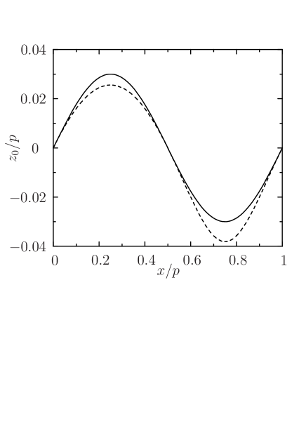
Figure 2: Comparison of the surface profiles given by Eq. (1) [solid line] and Eq. (5) [dashed line] for $A/p=0.03$.

II.3 Phase diagram

Figure 3 displays the phase diagram constructed as a function of the groove depth $A$ and the homeotropic anchoring strength $w_{H}$, for three values of the planar anchoring strength $w_{P}$. The textures P, T and H are separated by the lines of phase transitions which we refer to as the P-T, T-H and P-H transition, respectively. Both model ${\mathcal{A}}$ and ${\mathcal{B}}$ predict that the P-T transition is always continuous, whereas the T-H transition can be either first- or second-order, depending on the ratio $A/p$. We note, however, that the direct first-order P-H transition, which occurs when the grooves are sufficiently deep, follows only from model ${\mathcal{A}}$.

In the limit of small $w_{H}$ the planar texture is stable. When $w_{H}$ increases, and the grooves are shallow, the second-order P-T transition occurs. Our calculations show that for a fixed value of $w_{P}$ the location of this transition is rather independent of the groove depth, and when $w_{P}$ increases it moves towards larger values of $w_{H}$. For deeper grooves, the line of the continuous P-T transition terminates in a critical end point on the first-order T-H/P-H transition line. In the case of flat surface ($A=0$), the T-H transition is always continuous and can exist only for $pw_{P}/K\lesssim 9$. If $pw_{P}/K\gtrsim 9$ the H texture does not exist even for large values of $w_{H}$. For grating surfaces, the T-H transition changes from the second- to first-order when the groove depth increases. The change occurs at the tricritical point whose position shifts to higher values of $A$ upon decreasing $w_{P}$.

We emphasize that in our model of the NLC in contact with a chemically patterned but flat substrate ($A=0$) the phase transitions between the P or H texture and the T texture are always continuous, and there is no direct transition between the H and P textures. On the other hand, we observe a first-order P-H transition for a chemically uniform sinusoidal surface but for rather deep grooves ($A\gtrsim 0.25\,p$), similarly to the results obtained for asymmetric surface grating structures brow:00 . However, as it is apparent from Fig. 3, a combination of both chemical and geometrical surface pattern can lead to the first-order H-T transition, and also reduce the value of $A/p$ above which the H-P transition can be found. The repercussions of this result on possible bistable nematic devices are discussed in Sec. III. Note also that since the nematic texture induced by a periodic substrate is characterized by one of the effective anchoring directions: $\theta_{a}^{(eff)}=0$, $\theta_{a}^{(eff)}=\pi/2$ or $0<\theta_{a}^{(eff)}<\pi/2$, the observed phase transitions can be regarded as anchoring transitions.

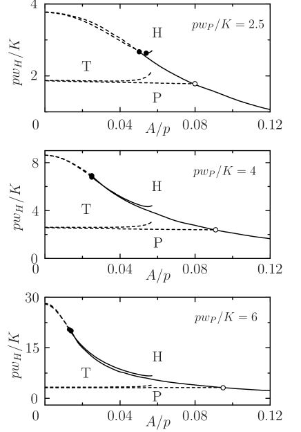
Figure 3: Phase diagram of a NLC in contact with a single sinusoidal grating surface [model ${\mathcal{A}}$, see Eq. (1) and Fig. 1] with alternating stripe pattern of locally planar and homeotropic anchoring as a function of groove depth $A$ and the strength of homeotropic anchoring $w_{H}$ for three values of the strength of planar anchoring $w_{P}$. The solid and the dashed lines denote first- and second-order transitions, respectively, between planar (P), tilted (T), and homeotropic (H) nematic textures. The solid and open circles mark tricritical and critical end points, respectively. For comparison, the results obtained from model ${\mathcal{B}}$ [see Eq. (4)] are shown with the same line code, but for $A<0.057\,p$.

In Fig. 3 we have also compared the predictions of models ${\mathcal{A}}$ and ${\mathcal{B}}$. We observe a good agreement for small values of $A/p$, whereas for deeper grooves some deviations appear. This reflects the fact that the difference between the grating profiles defined by Eqs. (1) and (4) becomes more pronounced with increasing groove depth. Since the application of model ${\mathcal{B}}$ is limited to rather small values of $A/p$, for the reasons already discussed, this model is unable to describe the first-order transition between the homeotropic and planar textures. However, the advantage of model ${\mathcal{B}}$ is that the precise determination of phase diagrams for small ratios $A/p$ becomes feasible, allowing one to study various aspects of the phase diagrams in more detail and with considerably less computational effort than within model ${\mathcal{A}}$. Thus, to obtain the overall picture of the phase transitions studied we have used information from both models.

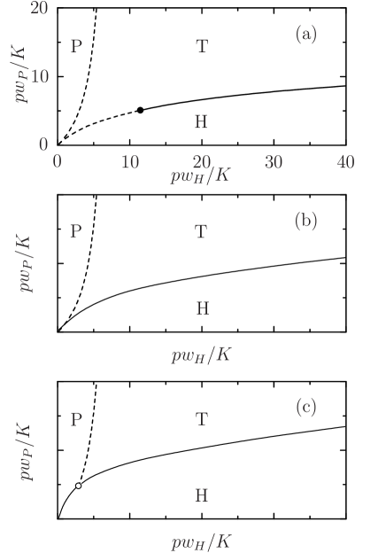
Figure 4: Phase diagram in the $\bm{(}pw_{H}/K,\,pw_{P}/K\bm{)}$ plane for: (a) $A<A_{0}$, (b) $A=A_{0}\approx 0.075\,p$ and (c) $A>A_{0}$. The meaning of symbols and lines is the same as in Fig. 3. Diagram (a) follows from the calculations based on model ${\mathcal{B}}$ for $A/p=0.02$. In the case of flat ($A=0$) chemically patterned substrate (not shown here) both phase transitions are continuous everywhere (the tricritical point on the H-T line escapes to $\infty$). Diagrams (b) and (c) correspond to model ${\mathcal{A}}$ but they are only schematic. At $A=A_{0}$ the tricritical point and the critical end point replace each other.

In Fig. 4, we present a sequence of phase diagrams in the $\bm{(}pw_{H}/K,\,pw_{P}/K\bm{)}$ plane, for three values of the groove depth: (a) $A<A_{0}$, (b) $A=A_{0}$ and (c) $A>A_{0}$, where $A_{0}/p\approx 0.075$. In all diagrams the P-T transition is continuous. In case (a), there is a tricritical point on the H-T transition line. For $A\to 0$ its position tends to the infinite value of $w_{H}$ (see Fig. 5), which is consistent with the flat substrate case. Upon increasing $A$ the tricritical point moves towards $\bm{(}pw_{H}/K=0,\,pw_{P}/K=0\bm{)}$ and eventually, at $A=A_{0}$ (case (b)), it reaches the origin, and the H-T transition becomes first-order everywhere. In case (c), the continuous P-T transition line does not extend to the origin, as in cases (a) and (b), but terminates at the first order transition line, which for $A>A_{0}$ consists of two pieces: the H-T and P-H lines. Note that when $A$ passes $A_{0}$ the tricritical point is replaced by the critical end point or vice versa.

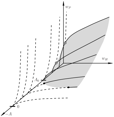
Figure 5: Three-dimensional phase diagram in the $\bm{(}pw_{P}/K,\,pw_{H}/K,\,A/p\bm{)}$ space. The meaning of symbols and lines is the same as in Fig. 3. The solid and dashed lines correspond to intersections with planes $A=const$, and the grey area corresponds to the surface of the first order transitions. Note the evolution of the tricritical point and the critical end point when $A/p$ changes.

To better visualize the relation between phase diagrams presented in Figs. 3 and 4, a schematic three-dimensional phase diagram in the space spanned by $\bm{(}pw_{P}/K,\,pw_{H}/K,\,A/p\bm{)}$ is also shown (see Fig. 5). The two-dimensional plots can be deduced from Fig. 5 by making intersections parallel to the plane $\bm{(}A/p,\,pw_{H}/K\bm{)}$ or $\bm{(}pw_{H}/K,\,pw_{P}/K\bm{)}$.

Finally we note that one can also consider the situation when homeotropic stripes are on the sides and planar stripes are on the hills (and in the pits) of the surface profile (see Fig. 1). In such a situation, the H-T transition line can be easily deduced from the P-T transition line of the above-discussed case by interchanging $w_{H}$ with $w_{P}$ and $p_{H}$ with $p_{P}$; the same holds for the line of the P-T phase transition.

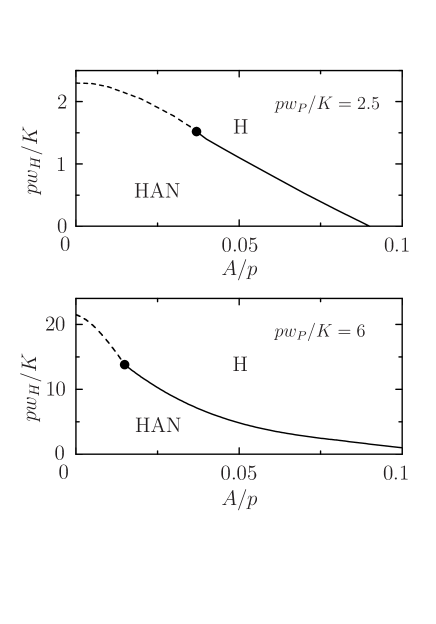
Figure 6: Phase diagram of a NLC confined between a patterned sinusoidal grating surface (see Fig. 1) and a flat surface with strong homeotropic anchoring as a function of groove depth $A$ and the strength of homeotropic anchoring $w_{H}$ for two values of the strength of planar anchoring $w_{P}$. The solid and dashed lines denote first- and second-order transitions, respectively, between a homeotropic (H) and hybrid aligned nematic (HAN) texture. The solid circles mark tricritical points. The width of the cell is $D/p=2$.

III Zenithally bistable nematic device

We now turn our attention to a NLC confined between a chemically patterned sinusoidal surface (which corresponds to model ${\mathcal{A}}$) and a flat substrate with strong homeotropic anchoring $\theta(x,D)=0$, where $D$ is the thickness of the cell. In the following calculations we keep $D$ fixed, but vary both the anchoring strengths and the groove depth at the grating surface. The numerical solution of the Euler–Lagrange equation demonstrates the existence of two nematic director configurations, namely the homeotropic (H) texture, where the director field is almost uniform and perpendicular to the flat surface, and the hybrid aligned nematic (HAN) texture, where the director field varies from homeotropic to nearly planar orientation through the cell (c.f. Fig. 7 below). Of course no planar texture, which exists in the semi-infinite case, can be found because of the strong homeotropic anchoring on the flat substrate.

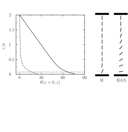
Figure 7: The tilt of the nematic director $\theta(x=0,z)$ with respect to the $z$-axis for a NLC confined between the patterned sinusoidal grating surface shown in Fig. 1 and a flat surface with strong homeotropic anchoring. The dashed and the solid lines represent the profile for the coexisting H and HAN textures for the planar anchoring strength $pw_{P}/K=2.45$ and groove depth $A/p=0.075$; see also the schematic nematic director profiles on the right side bar. The flat surface is located at $z=D=2p$ while the grating surface is at $z_{0}(x=0)=0$ (see Fig. 1). The location of the hills of the grating surface is marked by the dotted line.

Figure 6 displays the phase diagram plotted as a function of the groove depth $A$ and the homeotropic anchoring strength $w_{H}$ on the grating substrate for two values of the planar anchoring strength $w_{P}$ and for a fixed cell thickness $D$. For weak homeotropic anchoring the HAN texture is stable provided the groove depth is smaller than $A_{upp}$. For deeper grooves with $A>A_{upp}$ no HAN texture is found because distortions of the nematic director field are too costly in the presence of the dominating homeotropic anchoring. Upon increasing the groove depth, the HAN-H transition changes from second- to first-order at the tricritical point.

The tilt angle $\theta(x,z)$ in the middle of the planar stripe ($x=0$) is shown in Fig. 7 as a function of $z$ for the coexisting H and HAN textures. The nematic director is almost parallel to the $z$-axis in the H texture (for $z\gtrsim 0.6\,p$), while it changes smoothly from $\theta(0,z=D)=0$ to $\theta(0,z=0)<\pi/2$ in the HAN texture. In the latter case $\theta(0,z)$ decreases roughly linearly as the distance from the flat surface increases. Moreover, the numerical calculations exhibit that the nematic director field is rather independent of $x$ except of a thin surface layer (of width $\approx p/(2\pi)$) at the grating surface.

Finally, we emphasize that the groove depths for which zenithal bistability is found within the present model are considerably smaller than those considered theoretically ($A=0.8\,p$) parr:03 ; parr:04 and used experimentally ($A=0.35\,p$) brow:04 for a NLC confined between a pure geometrically patterned surface and a flat substrate parr:03 ; parr:04 . The calculated value of the average tilt of the nematic director just above the grating surface in the HAN texture is comparable to the one obtained in the case of the deeper grooves parr:03 ; parr:04 .

IV Summary

We have applied the Frank–Oseen model together with the Rapini–Papoular surface free energy to a NLC in contact with a single grating surface possessing an alternating stripe pattern of locally homeotropic and planar anchoring (Fig. 1) or confined between the patterned grating surface and a flat substrate. Phase diagrams and nematic director profiles are determined numerically with the following main results.

(1) A homeotropic, a planar, and a tilted nematic texture have been found for the NLC in contact with a single patterned grating surface (Figs. 3 - 5). Both second- and first-order transitions between the tilted texture and the homeotropic or planar texture are possible. Furthermore, for appropriate values of the groove depth and local anchoring strengths one can also observe a first-order transition between the homeotropic and planar textures. It is worthwhile to emphasize that the combination of chemical and geometrical surface pattern reduces the groove depth above which this transition occurs as compared to a pure geometrically patterned surface.

(2) For the NLC confined between a chemically patterned sinusoidal grating and a flat substrate which induces strong homeotropic anchoring, we have determined a first-order phase transition between a homeotropic texture and a hybrid aligned nematic texture for rather shallow grooves (Fig. 6). In the homeotropic texture, the nematic director is almost uniform and perpendicular to the flat surface, while the director field varies from homeotropic to nearly planar orientation in the hybrid aligned nematic texture (Fig. 7). Building on the results shown in Figs. 6 and 7 it seems possible to achieve a zenithally bistable nematic device without the use of a deep surface grating.

It is worthwhile to emphasize that not any combination of the chemical pattern and surface grating is capable of inducing first order transitions between the homeotropic and tilted textures or the homeotropic and planar textures in a semi-infinite NLC system. For instance, if the periods of the chemical pattern $\wp$ and of the surface grating $p$ are the same then the surface roughness merely changes the location of the second-order transitions observed in the flat substrate case, at least in the range of the groove depth studied in this work. Moreover, our numerical calculations suggest that the optimum ratio $p/\wp$ for the occurrence of the first order transitions in the case of relatively shallow grooves is $p/\wp=2$ shown in Fig. 1.

Finally, it is instructive to consider the situation when the chemical surface pattern is not exactly in phase with the surface grating profile. In such a case, for the reasons mentioned in Sec. II.1, there are no true homeotropic and planar textures, hence the accompanied second-order phase transitions cease to exist. However, first order transitions between a pseudo-homeotropic texture and the tilted or hybrid aligned texture should still exist, where the term pseudo-homeotropic means that the texture is characterized by $\theta_{a}^{(eff)}\approx 0$. Note also that the tricritical point in the phase diagrams shown in Figs. 3 - 6 becomes a critical point at which the difference between the pseudo-homeotropic and titled or hybrid aligned textures disappears.

References

- (1) D. W. Berreman, Phys. Rev. Lett. 26, 1683 (1972).
- (2) S. Faetti, Phys. Rev. A. 36, 408 (1987).
- (3) R. Barberi, M. Giocondo, G. V. Sayko, and A. K. Zvezdin, Phys. Lett. A 213, 293 (1996).
- (4) V. Mocella, C. Ferrero, M. Iovane, and R. Barberi, Liq. Cryst. 26, 1345 (1999).
- (5) J.-B. Fournier and P. Galatola, Phys. Rev. E. 60, 2404 (1999).
- (6) G. Barbero, G. Skačej, A. L. Alexe-Ionescu, and Žumer, Phys. Rev. E 60, 628 (1999)
- (7) C. V. Brown, M. J. Towler, V. C. Hui, and G. P. Bryan-Brown, Liq. Cryst. 27, 233 (2000).
- (8) P. Patrício, M. M. Telo da Gama, and S. Dietrich, Phys. Rev. Lett. 88, 245502 (2002).
- (9) D.-H. Chung, T. Fukuda, Y. Takanishi, K. Ishikawa, H. Matsuda, H. Takezoe, and M. A. Osipov, J. Appl. Phys. 92, 1841 (2002).
- (10) X. Lu, Q. Lu, Z. Zhu, J. Yin, and Zongguang Wang, Chem. Phys. Lett. 377, 433 (2003).
- (11) L. A. Parry-Jones, E. G. Edwards, S. J. Elston, and C. V. Brown Appl. Phys. Lett. 82, 1476 (2003).
- (12) C. V. Brown, L. A. Parry-Jones, S. J. Elston, and S. J. Wilkins, Mol. Cryst. Liq. Cryst. 410, 945 (2004).
- (13) L. A. Parry-Jones, E. G. Edwards, and C. V. Brown Mol. Cryst. Liq. Cryst. 410, 955 (2004).
- (14) E. E. Kriezis, C. J. P. Newton, T. P. Spiller, and S. J. Elston, Appl. Opt. 41, 5346 (2002).
- (15) H. L. Ong, A. J. Hurd, and R. B. Meyer, J. Appl. Phys. 57, 186 (1985).
- (16) G. Barbero, T. Beica, A. L. Alexe-Ionescu, and R. Moldovan, J. Phys. II France 2, 2011 (1992).
- (17) T. Z. Qian and P. Sheng, Phys. Rev. Lett. 77, 4564 (1996).
- (18) T. Z. Qian and P. Sheng, Phys. Rev. E 55, 7111 (1997).
- (19) V. K.Gupta and N. L. Abbott, Science 276, 1533 (1997).
- (20) B.-W. Lee and N. A. Clark, Science 291, 2576 (2001).
- (21) S. Kondrat and A. Poniewierski, Phys. Rev. E 64, 031709 (2001).
- (22) H. T. A. Wilderbeek, F. J. A. van der Meer, K. Feldmann, D. J. Broer, and C. W. M. Bastiaansen, Adv. Mater. 14, 655 (2002).
- (23) H. T. A. Wilderbeek, J.-P. Teunissen, C. W. M. Bastiaansen, and D. J. Broer, Adv. Mater. 15, 985 (2003).
- (24) S. Kondrat, A. Poniewierski, and L. Harnau, Eur. Phys. J. E 10, 163 (2003).
- (25) J.-H. Park, C.-J. Yu, J. Kim, S.-Y. Chung, and S.-D. Lee, Appl. Phys. Lett. 83, 1918 (2003).
- (26) B. Zhang, F. K. Lee, O. K. C. Tsui, and Ping Sheng, Phys. Rev. Lett. 21, 215501 (2003).
- (27) O. K. C. Tsui, F. K. Lee, B. Zhang, and Ping Sheng, Phys. Rev. E 69, 021704 (2004).
- (28) C.-J. Yu, J.-H. Park, J. Kim, M.-S. Jung, and S.-D. Lee, Appl. Opt. 43, 1783 (2004).
- (29) A. Poniewierski and S. Kondrat, J. Mol. Liq. 112, 61 (2004).
- (30) F. C. Frank, Discuss. Faraday Soc. 25, 19 (1958).
- (31) P. G. de Gennes and J. Prost, The Physics of Liquid Crystals (Clarendon, Oxford, 1993), 2nd ed.
- (32) A. Rapini and M. Papoular, J. Phys. (Paris) Colloq. 30, C4-54 (1969).
- (33) A. J. Davidson and N. J. Mottram, Phys. Rev. E 65, 051710 (2002).
- (34) S. Kondrat, A. Poniewierski, and L. Harnau, Liq. Cryst. 32, 95 (2005).
- (35) J. H. Lambert, Acta Helvetica 3, 128 (1758); J. H. Lambert, in Nouveaux mémories de l’Académie royale des science et belles-letteres (Berlin), volume 1; E. M. Wright, Proc. Royal Soc. Edinburgh A 62, 387 (1949); E. M. Wright, ibid 65, 193 (1959).
- (36) R. M. Corless, G. H. Gonnet, D. E. G. Hare, D. J. Jeffrey, and D. E. Knuth, Adv. Comput. Math. 5, 329 (1996).