Geometric Cluster Algorithm for
Interacting Fluids

Abstract

We discuss a new Monte Carlo algorithm for the simulation of complex fluids. This algorithm employs geometric operations to identify clusters of particles that can be moved in a rejection-free way. It is demonstrated that this geometric cluster algorithm (GCA) constitutes the continuum generalization of the Swendsen–Wang and Wolff cluster algorithms for spin systems. Because of its nonlocal nature, it is particularly well suited for the simulation of fluid systems containing particles of widely varying sizes. The efficiency improvement with respect to conventional simulation algorithms is a rapidly growing function of the size asymmetry between the constituents of the system. We study the cluster-size distribution for a Lennard-Jones fluid as a function of density and temperature and provide a comparison between the generalized GCA and the hard-core GCA for a size-asymmetric mixture with Yukawa-type couplings.

1 Introduction and Motivation

The presence of multiple time and length scales constitutes one of the major problems in computer simulations of matter. In simulations that faithfully capture the dynamic evolution of a system, the fastest particles in the system dictate the required time resolution. If different types of particles with widely varying diffusion rates are present, then the slower particles may be unable to explore the entire configuration space during the course of the simulation, leading to ergodicity problems.

In the computational study of complex fluids, such as colloidal suspensions, this problem frequently occurs, since such systems typically contain particles of different sizes. A concrete example is the ‘nanoparticle haloing’ phenomenon discovered by Lewis and coworkers tohver01 . This experimental work deals with a new approach to the stabilization of suspensions of micron-sized spherical particles, which tend to aggregate under the influence of their mutual van der Waals attraction. Conventional approaches to prevent this gelation, such as charge stabilization (variation of the pH to alter the surface charge of the particles), lead to complications in certain applications, e.g., in the formation of colloidal crystals, where the electrostatic repulsion prevents the close packing of the particles. It was found that these complications can be avoided by generating an effective colloidal repulsion through the addition of highly-charged nanometer-sized particles to the suspension of the (near-neutral) colloids. A concrete explanation for the underlying mechanism leading to the effective repulsions is currently lacking. Evidently, a computational approach to this problem must involve both the microspheres and the nanoparticles, which typically differ by a factor 100 in diameter. Traditionally, the effective pair interaction between colloids (potential of mean force) is then calculated by “integrating out” the smaller species, e.g., by simulating a system containing two spheres at fixed separation embedded in a sea of smaller particles dickman97 ; allahyarov98 . Here, we discuss a new simulation algorithm geomc that is capable of explicitly incorporating both species and computing equilibrium properties of the suspension, without suffering from the disparity in time scales. This algorithm can be viewed as a continuum version of the widely-used cluster algorithms for lattice spin models swendsen87 ; wolff89 .

2 Cluster Monte Carlo Algorithms

Equilibrium Monte Carlo methods are aimed at obtaining static thermodynamic and structural properties by generating system configurations according to the Boltzmann distribution. Nonphysical moves may be employed in the underlying Markov process, which – in principle – offers an exquisite way to overcome the presence of multiple time scales. Thus, Monte Carlo algorithms are the method of choice for, e.g., simulations of critical phenomena and phase transitions. In the context of size-asymmetric fluids, collective moves have been devised in which groups of particles are moved simultaneously. Unless these groups are identified in a careful way, which typically involves knowledge about the physical properties of the system, the Monte Carlo step will entail a large energy change and consequently have only a very small acceptance rate. Thus, while this approach has been used quite successfully in specific situations wu92 ; jaster99 ; woodcock99 ; lobaskin99 , it typically involves a tunable parameter and cannot be generalized in a straightforward fashion.

The situation is rather different for spin models, for which Swendsen and Wang (SW) swendsen87 introduced a cluster algorithm in which groups of parallel spins are identified in a probabilistic manner, based upon the Fortuin–Kasteleyn mapping of the Potts model onto the random-cluster model fortuin72 . These groups can subsequently be flipped independently. This rejection-free algorithm (every completed cluster can be flipped without an additional evaluation of the resulting energy difference) suppresses critical slowing down. Accordingly, its generalization to off-lattice fluids has been a widely-pursued goal. However, the SW algorithm – as well as the even more efficient single-cluster variant introduced by Wolff wolff89 – relies on invariance of the Hamiltonian under a spin-inversion operation. For a fluid, this translates into particle–hole symmetry, which is only obeyed for lattice gases. Consequently, efficient off-lattice cluster algorithms have only been designed for a small number of specific fluid models johnson97 ; sun00 , and it is not clear how these methods can be generalized. Hard-sphere fluids constitute another special case. Here every configuration without particle overlaps has the same energy. Dress and Krauth dress95 devised a strategy to create such configurations by means of geometric transformations. Their approach is particularly advantageous in size-asymmetric mixtures, but cannot be applied to systems with other interactions without supplementing it with a costly acceptance criterion. Nevertheless, a remarkable feature of this geometric cluster algorithm is that it relies on the invariance of the Hamiltonian under geometric operations. Here, we exploit this property to formulate a cluster Monte Carlo algorithm that is applicable to arbitrary pair potentials without the imposition of an acceptance criterion.

3 Generalized Geometric Cluster Algorithm

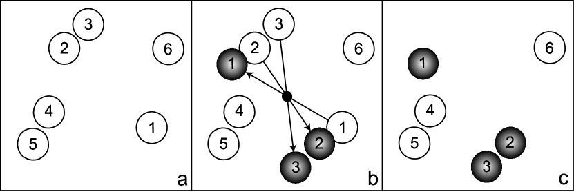
Figure 1: Two-dimensional illustration of the interacting geometric cluster algorithm. Open and shaded circles label the particles before and after the geometrical operation, respectively. The small filled disk denotes the pivot. a) Initial configuration; b) construction of a new cluster via point reflection of particles $1$–$3$ with respect to the pivot; c) final configuration.

3.1 Single-cluster variant

The geometric cluster algorithm as formulated by Dress and Krauth starts from a configuration of particles, with periodic boundary conditions. This configuration is rotated around an arbitrarily chosen pivot. Groups of particles that overlap between the original and the rotated configuration are exchanged between these configurations. In practice, it is more convenient to construct only a single cluster and to carry out a point reflection on the fly heringa98 . For each cluster a new pivot is chosen. This constitutes the counterpart of the Wolff algorithm for spin models wolff89 . In the presence of a general, isotropic pair potential $V(r)$ the cluster construction proceeds as follows (cf. Fig. 1):

1. Choose a random pivot point.

2. Choose the first particle $i$ at random and move it from its original position $\mathbf{r}_{i}$ to its new position $\mathbf{r}_{i}^{\prime}$, via a point reflection with respect to the pivot.

3. Identify all particles that interact with $i$ in its original position or in its new position. These particles $j$ are considered for a point reflection with respect to the pivot. This reflection is carried out with a probability $p_{ij}=\max[1-\exp(-\beta\mbox{{D}}_{ij}),0]$, where $\mbox{{D}}_{ij}=V(|\mathbf{r}_{i}^{\prime}-\mathbf{r}_{j}|)-V(|\mathbf{r}_{i}-\mathbf{r}_{j}|)$ and $\beta=1/k_{\rm B}T$. Note that $p_{ij}$ solely depends on the interaction strength between $i$ and $j$.

4. Repeat step 3 in an iterative fashion for each particle $j$ that is added to the cluster. If $j$ is moved with respect to the pivot, then all its interacting neighbors that have not yet been added to the cluster are considered for inclusion as well. The cluster construction is completed once all interacting neighbors have been considered.

It is instructive to compare this prescription to the Wolff cluster algorithm, in which a cluster of parallel spins is grown from a randomly chosen initial spin. Parallel spins with a ferromagnetic coupling constant $K$ are added to the cluster with a probability $1-\exp(-2K)$. The energy difference between the parallel and the antiparallel configuration indeed equals $2K$. An antiparallel spin is never added to the cluster, in accordance with the fact that such a pair will be in a state of lower energy if only the first spin is flipped.

This algorithm is ergodic, since each particle can be moved over an arbitrarily small distance. Namely, there is a non-vanishing probability that a cluster consists of only a single particle and the pivot can be located arbitrarily close to the center of this particle. Detailed balance is proven by considering a configuration $X$ which is transformed into a new configuration $Y$ by means of a cluster move. The energy change $E_{Y}-E_{X}$ results from every particle that is not included in the cluster but interacts with one or more particles that are part of the cluster. Each “broken bond” has a probability $1-p_{k}$, so that the total probability of forming a cluster is given by

$$T(X\to Y)=C\prod_{k}(1-p_{k})\;.$$ (1)

The prefactor $C$ accounts for the probability of choosing a specific pivot and for the probability of creating a specific arrangement of bonds inside the cluster. The total set $\{k\}$ of broken bonds can be divided into two subsets. The broken bonds $l$ that lead to an increase $\mbox{{D}}_{l}$ in pair energy have a probability $\exp(-\beta\mbox{{D}}_{l})$, whereas the broken bonds $m$ that lead to a decrease in pair energy have a probability equal to unity. Accordingly, the transition probability can be written as

$$T(X\to Y)=C\exp\left[-\beta\sum_{l}\mbox{{D}}_{l}\right]\;.$$ (2)

The reverse move, in which the configuration $Y$ is transformed into the configuration $X$ by moving a cluster that is constructed in the same way, has a probability

$$T(Y\to X)=C\prod_{k}(1-\bar{p}_{k})\;,$$ (3)

where the sum runs over the same set $\{k\}$ of broken bonds as in Eq. (1), but the sign of all energy differences $\mbox{{D}}_{k}$ has been reversed (indicated by $\bar{p}_{k}$). Accordingly, the sum over $\mbox{{D}}_{l}$ in Eq. (2) is replaced by the negative sum over the complementary set $\{m\}$,

$$T(Y\to X)=C\exp\left[+\beta\sum_{m}\mbox{{D}}_{m}\right]\;.$$ (4)

The point reflection is a self-inverse operation, so that detailed balance is obeyed without the need to impose an acceptance criterion:

$$\frac{T(X\to Y)}{T(Y\to X)}=\exp\left[-\beta\sum_{k}\mbox{{D}}_{k}\right]=\frac{\exp(-\beta E_{Y})}{\exp(-\beta E_{X})}\;.$$ (5)

Since energy differences are taken into account on a pair-wise basis during the construction of the cluster, rather than as a total energy difference after the cluster has been completed, the cluster is constructed in such a way that large energy differences are avoided. The clusters are representative of the actual structure of the system.

3.2 Multiple-cluster variant

In order to demonstrate that the generalized geometric cluster algorithm (GCA) indeed constitutes the off-lattice counterpart of the SW and Wolff cluster algorithms, it is instructive to formulate a multiple-cluster variant. This formulation yields a full decomposition of an off-lattice fluid configuration into stochastically independent clusters. In the following, we demonstrate how it can be phrased as a natural extension of the single-cluster version.

First, a cluster is constructed according to the Wolff version of the GCA, with the exception that the cluster is only identified; particles belonging to the cluster are marked but not actually moved. The chosen pivot will also be used for the construction of all subsequent clusters in this decomposition. These subsequent clusters are built just like the first cluster, except that particles that are already part of an earlier cluster will never be considered for a new cluster. Once each particle is part of a cluster the decomposition is completed and each cluster is moved with a probability $f$.

Although all clusters except the first are built in a restricted fashion, every individual cluster is constructed according to the rules of the Wolff formulation of the GCA. The exclusion of particles that are already part of another cluster simply reflects the fact that every bond should be considered only once. If a bond is broken during the construction of an earlier cluster it must not be re-established during the construction of a subsequent cluster.

In order to establish that this prescription is a true equivalent of the SW algorithm, we prove that each cluster can be moved (reflected) independently while preserving detailed balance. If only a single cluster is actually moved, this essentially corresponds to the Wolff version of the GCA, since each cluster is built according to the GCA prescription. The same holds true if several clusters are moved and no interactions are present between particles that belong to different clusters (the hard-sphere algorithm is a particular realization of this situation). If two or more clusters are moved and broken bonds exist between these clusters, i.e., a non-vanishing interaction exists between particles that belong to disparate (moving) clusters, then the shared broken bonds are actually preserved and the proof of detailed balance provided in the previous section no longer applies in its original form. However, since these bonds are identical in the forward and reverse move, the corresponding factors cancel out. This is illustrated for the situation of two clusters whose construction involves, respectively, two sets of broken bonds $\{k_{1}\}$ and $\{k_{2}\}$. Each set comprises bonds $l$ that lead to an increase in pair energy and bonds $m$ that lead to a decrease in pair energy. We further subdivide these sets into external bonds that connect cluster 1 or 2 with the remainder of the system and joint bonds that connect cluster 1 and 2. Accordingly, the probability of creating cluster 1 is given by

$$C_{1}\prod_{i\in\left\{l_{1}\right\}}(1-p_{i})=C_{1}\prod_{i\in\left\{l_{1}^{\rm ext}\right\}}(1-p_{i})\prod_{j\in\left\{l_{1}^{\rm joint}\right\}}(1-p_{j})\;.$$ (6)

Upon construction of the first cluster, the creation of the second cluster has a probability

$$C_{2}\prod_{i\in\left\{l_{2}^{\rm ext}\right\}}(1-p_{i})\;,$$ (7)

since all joint bonds in $\{l_{1}^{\rm joint}\}$ already have been broken. The factors $C_{1}$ and $C_{2}$ account for the probability of realizing a particular arrangement of internal bonds in clusters 1 and 2, respectively. Hence, the total transition probability for moving both clusters (upon fixing the pivot) is given by

$$T_{12}=C_{1}C_{2}\exp\left[-\beta\sum_{i\in\left\{l_{1}^{\rm ext}\right\}}\mbox{{D}}_{i}-\beta\sum_{j\in\left\{l_{2}^{\rm ext}\right\}}\mbox{{D}}_{j}-\beta\sum_{n\in\left\{l_{1}^{\rm joint}\right\}}\mbox{{D}}_{n}\right]\;.$$ (8)

In the reverse move, the energy differences for all external broken bonds have changed sign, but the energy differences for the joint bonds connecting cluster 1 and 2 are the same as in the forward move. Thus, cluster 1 is created with probability

$$C_{1}\prod_{i\in\left\{m_{1}^{\rm ext}\right\}}(1-\bar{p}_{i})\prod_{j\in\left\{l_{1}^{\rm joint}\right\}}(1-p_{j})$$ (9)

$$= C_{1}\prod_{i\in\left\{m_{1}^{\rm ext}\right\}}\exp[+\beta\mbox{{D}}_{i}]\prod_{j\in\left\{l_{1}^{\rm joint}\right\}}\exp[-\beta\mbox{{D}}_{j}]\;,$$

where the $\bar{p}$ reflects the sign change compared to the forward move and the product over the external bonds involves the complement of the set $\{l_{1}^{\rm ext}\}$. The creation probability for the second cluster is

$$C_{2}\prod_{i\in\left\{m_{2}^{\rm ext}\right\}}(1-\bar{p}_{i})=C_{2}\prod_{i\in\left\{m_{2}^{\rm ext}\right\}}\exp[+\beta\mbox{{D}}_{i}]$$ (10)

and the total transition probability for the reverse move is

$$\tilde{T}_{12}=C_{1}C_{2}\exp\left[+\beta\sum_{i\in\left\{m_{1}^{\rm ext}\right\}}\mbox{{D}}_{i}+\beta\sum_{j\in\left\{m_{2}^{\rm ext}\right\}}\mbox{{D}}_{j}-\beta\sum_{n\in\left\{l_{1}^{\rm joint}\right\}}\mbox{{D}}_{n}\right]\;.$$ (11)

Accordingly, detailed balance is still fulfilled,

$$\frac{T_{12}}{\tilde{T}_{12}}=\exp\left[-\beta\sum_{i\in\left\{k_{1}^{\rm ext}\right\}}\mbox{{D}}_{i}-\beta\sum_{j\in\left\{k_{2}^{\rm ext}\right\}}\mbox{{D}}_{j}\right]=\exp\left[-\beta(E_{Y}-E_{X})\right]\;,$$ (12)

in which $\{k_{1}^{\rm ext}\}=\left\{l_{1}^{\rm ext}\right\}\cup\left\{m_{1}^{\rm ext}\right\}$ and $\{k_{2}^{\rm ext}\}=\left\{l_{2}^{\rm ext}\right\}\cup\left\{m_{2}^{\rm ext}\right\}$ and $E_{X}$ and $E_{Y}$ refer to the total internal energy before and after the move, respectively. This treatment applies to any simultaneous move of clusters, so that each cluster in the decomposition indeed can be moved independently without violating detailed balance. It is noteworthy that the probabilities for breaking joint bonds in the forward and reverse moves cancel only because the probability in the cluster construction factorizes into pairwise probabilities, as opposed to the probability for a multiple-particle move in a Metropolis-type algorithm.

Figure 2: Comparison between the single-cluster version (solid lines) and the multiple-cluster version (symbols) of the generalized geometric cluster algorithm. The figure shows pair correlation functions for the size-asymmetric Lennard-Jones mixture described in Ref. geomc . The system contains $800$ small (diameter $\sigma$) and $400$ large particles (diameter $5\sigma$) at a total packing fraction $\eta\approx 0.213$. $g_{\textrm{ll}}$ and $g_{\textrm{ls}}$ represent the large–large and large–small correlation functions, respectively.

As demonstrated in Fig. 2 for a binary mixture, the results obtained by means of the multiple-cluster geometric algorithm agree perfectly with those obtained using the single-cluster version.

4 Performance

The most striking feature of the generalized geometric cluster algorithm, apart from the fact that it creates clusters that can be moved in a rejection-free manner, is the speed at which it relaxes size-asymmetric mixtures. We illustrate this here for a binary fluid mixture consisting of $N_{\rm s}$ small and $N_{\rm l}$ large spherical particles with size ratio $\alpha\equiv\sigma_{\rm l}/\sigma_{\rm s}>1$. The particles are contained in a fixed volume, at equal packing fractions $\eta_{\rm s}=\eta_{\rm l}=0.1$. While $N_{\rm l}=150$ is kept fixed, $N_{\rm s}$ increases from $1\,200$ to $506\,250$ as $\alpha$ is varied from $2$ to $15$. Pairs of small particles and pairs involving a large and a small particle act like hard spheres. However, in order to prevent depletion-driven aggregation of the large particles, they have a Yukawa repulsion,

$$U_{22}(r)=\left\{\begin{array}[]{ll}+\infty&\quad r\leq\sigma_{\rm l}\\ J\exp[-\kappa(r-\sigma_{\rm l})]/(r/\sigma_{\rm l})&\quad r>\sigma_{\rm l}\;,\end{array}\right.$$ (13)

where $\beta J=3.0$ and the screening length $\kappa^{-1}=\sigma_{\rm s}$. In the simulation, the exponential tail is cut off at $3\sigma_{\rm l}$. As a measure of efficiency we consider the integrated autocorrelation time $\tau$ obtained from the energy autocorrelation function binder01 ,

$$C(t)=\frac{\langle{E(0)E(t)}\rangle-{\langle{E(0)}\rangle}^{2}}{\langle{E(0)^{2}}\rangle-{\langle{E(0)}\rangle}^{2}}\;.$$ (14)

For conventional MC calculations, $\tau$ rapidly increases with increasing $\alpha$, because the large particles tend to get trapped by the small particles. Accordingly, an accurate estimate for $\tau$ could only be obtained for $\alpha\leq 7$. By contrast, the generalized GCA has an autocorrelation time that only weakly depends on the size ratio, as illustrated in Fig. 3. At $\alpha=7$ the resulting efficiency gain already amounts to more than three orders of magnitude.

Figure 3: Efficiency comparison between a conventional local update algorithm (open symbols) and the generalized geometric cluster algorithm (closed symbols), for a binary mixture (see text) with size ratio $\alpha$. Whereas the autocorrelation time per particle (expressed in $\mu$s of CPU time per particle move) rapidly increases with size ratio, the GCA features only a weak dependence on $\alpha$.

(a)

(b)

Figure 4: Cluster size distributions as a function of relative cluster size $X$, for a monodisperse Lennard-Jones fluid. (a) Reduced density $\rho^{*}\equiv\rho\sigma^{3}=0.32$; (b) reduced density $\rho^{*}=0.16$. Identical symbols compare to identical temperatures in both panels. All temperatures are indicated in terms of $\varepsilon/k_{\rm B}$. See text for discussion.

A crucial limitation of the generalized GCA is that each cluster must only occupy a fraction of the entire system. As observed by Dress and Krauth dress95 , the entire system typically will be occupied by a single cluster once the percolation threshold is reached in the combined system containing a configuration and its point-reflected counterpart. For the original system this leads, in three dimensions, to a practical upper limit in the packing fraction around $0.23$–$0.25$. This number will vary as a function of size asymmetry and, if additional pair interactions are present, temperature. It is therefore instructive to study the cluster-size distribution as a function of reduced density $\rho^{*}$ and temperature $T$. Figure 4 illustrates the cluster-size distributions as obtained by means of the multiple-cluster GCA for a regular (one-component) Lennard-Jones fluid. In the top panel, $\rho^{*}=0.32\approx\rho^{*}_{\rm c}$. Already at temperatures that are far above the critical temperature $T_{\rm c}\approx 1.19$, the cluster-size distribution starts to tend toward a bimodal form, indicative of the formation of large clusters. In the vicinity of the critical temperature, the average cluster size has become very large. For comparison, the bottom panel displays the cluster-size distributions at a twice smaller density, $\rho^{*}=0.16$. In this case the bimodal shape does not appear until close to $T_{\rm c}$.

The properties suggest that the generalized GCA, at least for the one-component Lennard-Jones fluid, will not suppress critical slowing – the primary advantage of lattice cluster algorithms. For the off-lattice GCA, this property is less essential, because of the speed-up it delivers for the simulation of size-asymmetric fluids over a wide range of temperatures and packing fractions. Nevertheless, we have investigated the integrated autocorrelation time for the energy at the critical point, as a function of linear system size. In Fig. 5 these times are collected for three algorithms. (1) Conventional local-update Metropolis algorithm; (2) Wolff version of the GCA; (3a) SW version of the GCA, in which each cluster is reflected with a probability $0.50$; (3b) SW version of the GCA, in which each cluster is reflected with a probability $0.75$. Just as for spin models, the single-cluster version outperforms the Swendsen–Wang type cluster decompositions. However, all variants of the GCA exhibit the same power-law behavior, which outperforms the Metropolis algorithm by a factor $\sim L^{2.1}$. It is important to emphasize that this acceleration may be due to the suppression of the hydrodynamic slowing down hohenberg77

Figure 5: Energy autocorrelation time $\tau$ as a function of linear system size for a critical Lennard-Jones fluid, in units of particle sweeps, for three different Monte Carlo algorithms: Local moves (“Metropolis MC”); GCA with Swendsen–Wang type cluster decomposition and probability 0.50 (“SW 50%”) and 0.75 (“SW 75%”) of moving each cluster; single-cluster GCA (“Wolff”).

caused by the conservation of the density (which may couple to the energy correlations geomc ). Another striking point is that already for moderate system sizes the generalized GCA outperforms the Metropolis algorithm, despite the time-consuming construction of large clusters [cf. Fig. 4(a)] which only lead to small configurational changes.

Figure 6: Pair correlation function of dilute colloidal particles (diameter $\sigma$) in an environment of smaller particles (diameter $\sigma/5$, packing fraction $\eta=0.116$) that experience a Yukawa-type attractive interaction with the colloids. The symbols represent data obtained by means of the hard-core GCA malherbe99 ; the solid line was obtained from the generalized GCA.

5 Illustration

In order to illustrate the capabilities of the generalized GCA, we have computed the pair correlation function of dilute colloidal particles (packing fraction $\eta_{\rm l}=0.001$) in an environment of particles with a five times smaller diameter (packing fraction $\eta_{\rm s}=0.116$). Large and small particles act as hard spheres, but unlike pairs (i.e., large–small) experience a Yukawa attraction which promotes the accumulation of small particles around the colloids. This system has been studied in Ref. malherbe99 by means of the original hard-core GCA, in which clusters are moved according to an acceptance criterion, as proposed in Ref. dress95 . This potentially greatly deteriorates performance, as entire clusters will be constructed that are subsequently rejected. Indeed, the authors report malherbe99 that the colloid pair correlation function $g(r)$ had to be obtained via numerical differentiation of the integrated pair correlation function, rather than through direct sampling. The generalized GCA can handle this system without complication, as demonstrated in Fig. 6. In order to obtain data comparable to the solid curve in this figure, the authors of Ref. malherbe99 utilized a polynomial fit to the integrated pair correlation function, which potentially leads to ambiguities.

6 Conclusion and Outlook

We have discussed the generalized geometric cluster algorithm, a Monte Carlo method for the simulation of fluids by means of geometric operations. This algorithm creates nonlocal multiple-particle moves that are capable of rapidly decorrelating fluid configurations that contain particles of widely different sizes. The multiple-particle moves are constructed in such a way that the typical decrease in acceptance rate is avoided; every proposed move is accepted without violating detailed balance. It is anticipated that this algorithm will find widespread application, in particular in the simulation of complex fluids and suspensions in which the solvent is modeled as an implicit background. Potential generalizations include the treatment of particles with internal degrees of freedom, such as nonspherical particles, and other geometries, such as layered systems.

References

- (1) V. Tohver, J. E. Smay, A. Braem, P. V. Braun, and J. A. Lewis, Proc. Natl. Acad. Sci. U.S.A. 98, 8950 (2001).
- (2) R. Dickman, P. Attard, and V. Simonian, J. Chem. Phys. 107, 205 (1997).
- (3) E. Allahyarov, I. D’Amico, and H. Löwen, Phys. Rev. Lett. 81, 1334 (1998).
- (4) J. Liu and E. Luijten, Phys. Rev. Lett. 92, 035504 (2004).
- (5) R. H. Swendsen and J.-S. Wang, Phys. Rev. Lett. 58, 86 (1987).
- (6) U. Wolff, Phys. Rev. Lett. 62, 361 (1989).
- (7) D. Wu, D. Chandler, and B. Smit, J. Phys. Chem. 96, 4077 (1992).
- (8) A. Jaster, Physica A 264, 134 (1999).
- (9) L. Lue and L. V. Woodcock, Mol. Phys. 96, 1435 (1999).
- (10) V. Lobaskin and P. Linse, J. Chem. Phys. 111, 4300 (1999).
- (11) C. M. Fortuin and P. W. Kasteleyn, Physica 57, 536 (1972).
- (12) G. Johnson, H. Gould, J. Machta, and L. K. Chayes, Phys. Rev. Lett. 79, 2612 (1997).
- (13) R. Sun, H. Gould, J. Machta, and L. W. Chayes, Phys. Rev. E 62, 2226 (2000).
- (14) C. Dress and W. Krauth, J. Phys. A 28, L597 (1995).
- (15) J. R. Heringa and H. W. J. Blöte, Phys. Rev. E 57, 4976 (1998).
- (16) K. Binder and E. Luijten, Phys. Rep. 344, 179 (2001).
- (17) P. C. Hohenberg and B. I. Halperin, Rev. Mod. Phys. 49, 435 (1977).
- (18) J. G. Malherbe and S. Amokrane, Mol. Phys. 97, 677 (1999).