Raman resonance in spin $S$ two-leg ladder systems

Abstract

We argue that the Raman intensity in a spin $S$ two-leg spin-ladder has a pseudo-resonance peak, whose width is very small at large $S$. The pseudo-resonance originates from the existence of a local minimum in the magnon excitation spectrum, and is located slightly below twice the magnon energy at the minimum. The physics behind the peak is similar to the excitonic scenario for the neutron and Raman resonances in a $d-$wave superconductor.

Recently, there has been a considerable experimental progress in Raman studies of two-leg spin-ladder materials $(Sr,La)_{14}Ca_{x}Cu_{24}O_{41}$ (Ref girsh ; sugai ) and $SrCu_{2}O_{3}$ Thomsen . The most intriguing experimental result is the discovery of a sharp peak in the Raman intensity of $Sr_{14}Cu_{24}O_{41}$ at a frequency near $3000cm^{-1}$ (about $400meV$). The peak exists for polarizations of incoming and outgoing light both along and across the ladders ($xx$ and $yy$, respectively), and its width for xx polarization is around $130cm^{-1}$ which is nearly 10 times smaller than the width of the two-magnon peak in 2D antiferromagnets girsh .

The discovery of the peak stimulated the search for possible resonance-like features in the two-magnon Raman profile $R(\omega)$ of spin-ladder systems  uhrig ; Trebst ; uhrig_2 ; FreitasSingh . Previous studies of $S=1/2$ ladders didn’t find the resonance and suggested more complex explanation of the sharp peak in $R(\omega)$ uhrig ; uhrig_2 . We argue in this paper that the Raman intensity in a spin $S$ two-leg ladder possesses a pseudo-resonance, whose origin is similar to the origin of the neutron resonance and $B_{1g}$ Raman pseudo-resonance in high $T_{c}$ superconductors neutrons ; cmb . The intrinsic width of the Raman resonance is small in $1/S$ for $S\gg 1$, but increases as $S$ decreases. We discuss whether the sharp Raman peak observed in $S=1/2$ material $Sr_{14}Cu_{24}O_{41}$ may be this resonance.

The pseudo-resonance in a two-leg ladder emerges because of the existence of a local minimum in the magnon spectrum. The magnetic excitations in a ladder are well described by Heisenberg interactions between spins along the legs of the ladder ($J_{1}$) and along the rungs of the ladder ($J_{2}$). In the quasiclassical (large $S$) approximation, the excitation spectrum consists of two branches $\epsilon_{k}$ and $\epsilon_{k+\pi}$ where

$$\epsilon_{k}=4J_{1}S|\sin(k/2)|\sqrt{\cos^{2}(k/2)+J_{2}/2J_{1}}.$$ (1)

The spectrum $\epsilon_{k}$ is gapless at $k=0$, and for $J_{2}<2J_{1}$, which we only consider, it reaches a maximum $\epsilon_{max}=S(2J_{1}+J_{2})$ at some finite $k$, then falls down and reaches a minimum $\epsilon_{min}=S\sqrt{8J_{1}J_{2}}$ at $k=\pi$ (see Fig.1a). At a finite $S$, Haldane effect haldane produces a gap in $\epsilon_{k}$ at $k=0$ uhrig , however, the minimum at $k=\pi$ survives (see Fig.1b). We verified that the effects on the Raman profile from $\epsilon_{k}$ and $\epsilon_{k+\pi}$ are additive, so below we only discuss the dispersion branch $\epsilon_{k}$

Figure 1: The magnon excitation spectrum in a two-leg ladder. Left panel, the quasiclassical case $S\gg 1$, $J_{2}/J_{1}=0.4$. Right panel - schematic $\epsilon_{k}$ for $S=1/2$ uhrig . In both cases, the spectrum has a local minimum at $k=\pi$ and a local maximum at some smaller $k$. In the quasiclassical case, the excitation spectrum is gapless at $k=0$. For $S=1/2$ ladder, magnon states near $k=0$ are gapped due to the Haldane effect. Note that our momenta are shifted by $\pi$ compared to uhrig . The local minimum disappears at $J_{2}/J_{1}=2$ both in the quasiclassical case and for $S=1/2$ Trebst

We first present the summary of the results and then discuss the computations. Following previous studies of $2D$ systems singh ; cf , we assume that the Raman intensity $R(\omega)$ in two-leg ladders is reasonably well approximated by the RPA expression rpa

$$R(\omega)=-\frac{ImR_{0}}{\left(1+aReR_{0}\right)^{2}+\left(aImR_{0}\right)^{2}},$$ (2)

where $R_{0}(\omega)$ is the polarization bubble of free fermions with Raman vertices, and positive $a$ accounts for magnon-magnon interaction. Near $\epsilon_{min}$ and $\epsilon_{max}$, excitation spectrum is flat, and the magnon density of states diverges. This leads to square-root singularities in $R_{0}(\omega)$ near $2\epsilon_{min}$ and $2\epsilon_{max}$. Near these two singularities,

$$R_{0}(\omega)=-\frac{A}{\sqrt{2\epsilon_{min}-\omega-i\delta}}~{}~{}R_{0}(\omega)=\frac{A^{*}}{\sqrt{\omega-2\epsilon_{max}+i\delta}},$$ (3)

where $A$ and $A^{*}$ are positive. The imaginary part of $R_{0}(\omega)$ diverges at approaching $2\epsilon_{min}$ from above and at approaching $2\epsilon_{max}$ from below (see Fig. 2). One can easily make sure that in both cases $ImR_{0}$ is negative (and Raman intensity is positive). Meanwhile, $ReR_{0}(\omega)$ is positive above $2\epsilon_{max}$, and negative below $2\epsilon_{min}$ (see Fig. 2). A positive $ReR_{0}(\omega)$ at $\omega>2\epsilon_{max}$ implies that above $2\epsilon_{max}$, $1+aReR_{0}(\omega)$ in Eq. (2) is far from zero, i.e., there is no antibound state in the Raman profile. This is consistent with previous studies of the Raman profile in 2D Heisenberg systems cf . At the same time, below $2\epsilon_{max}$, $ReR_{0}(\omega)<0$, and therefore there exists a frequency $\omega_{res}$ at which $1+aReR_{0}(\omega_{res})=0$, and the Raman intensity $R(\omega)$ is strongly enhanced. If $\epsilon_{min}$ was a true minimum of the excitation spectrum, the full $R(\omega)$ given by Eq. (2) would develop a truly $\delta-$functional resonance peak at $\omega=\omega_{res}$. In reality, there are magnon states below $\epsilon_{min}$ (see Fig.2), and $ImR_{0}$ remains finite, albeit small below $2\epsilon_{min}$. In this situation, the full Raman intensity acquires only a peak at $\omega=\omega_{0}$. The width of the peak scales as $1/S$ at large $S$, but is $O(1)$ for $S=1/2$ (see Fig.3).

Figure 2: The behavior of the Raman bubble $R_{0}(\omega)$ (in units of $J_{1}$ for non-interacting magnons. We used $J_{2}/J_{1}=0.8$ for illustrative purposes. Near $2\epsilon_{max}$ and $2\epsilon_{min}\approx 1.8\epsilon_{max}$, the polarization bubble diverges as a square-root due to singularities in the magnon density of states. Observe that while $ImR_{0}(\omega)$ is negative for all frequencies, $ReR_{0}(\omega)$ is positive above $2\epsilon_{max}$, but negative below $2\epsilon_{min}$. This last behavior leads to a resonance in the Raman intensity below $2\epsilon_{min}$. In between $1.8\epsilon_{max}$ and $2\epsilon_{max}$, $ReR_{0}(\omega)$ is nonzero, but very small.

The physics that we just described is very similar to the excitonic scenario for the resonance in the neutron scattering  neutrons and the pseudo-resonance in $B_{1g}$ Raman intensity cmb in the cuprates. Like in cuprates, the resonance in the two-leg ladders is the combination of the two effects: the presence of the gap in a single particle excitation spectrum, and the attractive residual interaction between quasiparticles. The attraction leads to a formation of a two-particle bound state below twice the gap, which shows up as a resonance in $R(\omega)$. The finite intrinsic width of the Raman resonance in a ladder is due to the fact that Raman intensity is a $q=0$ probe, and it includes a contribution from the states for which $ImR_{0}(\omega)$ is finite below $2\epsilon_{min}$.

Figure 3: The theoretical behavior of the full Raman intensity $R(\omega)$ given by Eq. (2). Left panel, the quasiclassical case formally extended to $S=1/2$. Solid line is the result of numerical calculations valid at large $\omega$, near twice minimum and maximum of the magnon spectrum. Dashed line is the expected behaviour for small $\omega.$ We used $J_{2}/J_{1}=0.8$, as in Fig.2. Right panel, the expected behavior of $R(\omega)$ for $S=1/2$. The width of the pseudo-resonance below $2\epsilon_{min}$, obtained in numerical simulations for $S=1/2$ ladder uhrig ; uhrig_2 , is larger than in the quasiclassical analysis extended to $S=1/2$.

In $Sr_{14}Cu_{24}O_{41}$, the sharp peak in the Raman profile has been detected around $3000cm^{-1}$  girsh ; sugai . The measured maximum frequency $2\epsilon_{max}$ is near $4000cm^{-1}$. Whether or not this peak is our pseudo-resonance depends on whether this material is truly described by a $S=1/2$ ladder, or Haldane effect is suppressed by $3D$ couplings, and the form of the excitation spectrum is similar to the quasiclassical expression. In the first case, numerical studies indicate uhrig ; uhrig_2 that the pseudo-resonance is too broad to account for the data. However, if the quasiclassical description is valid down to $S=1/2$, the pseudo-resonance below $2\epsilon_{min}=2\sqrt{2J_{1}J_{2}}$ is quite sharp (Fig.3a) and the profile of $R(\omega)$ is consistent with the data. Matching the peak position and the location of the upper edge for $R(\omega)$ by quasiclassical formulas yields $J_{1}\sim 1600cm^{-1}$ ($200meV$) and $J_{2}/J_{1}\sim 0.4-0.5$. This value of $J_{1}$ is comparable to $J\sim 100meV$ in the 2D cuprates  2d_exchange , the value of $J_{2}/J_{1}$ roughly agrees with other estimates girsh ; FreitasSingh .

In the rest of the paper we present the details of our derivation of the Raman intensity. Our point of departure is the Hubbard Hamiltonian for two chains

$$H = -t\sum_{<i,j>}(c^{\dagger}_{i,\sigma}c_{j,\sigma}+d^{\dagger}_{i,\sigma}d_{j,\sigma})-t^{\prime}\sum_{i}c^{\dagger}_{i,\sigma}d_{i,\sigma}+h.c.$$ (4)

$$+U\sum_{i}\left(n_{i,\uparrow}^{c}n_{i,\downarrow}^{c}+n_{i,\uparrow}^{d}n_{i,\downarrow}^{d}\right).$$

In the quasiclassical case, we introduce antiferromagnetic long-range order at $Q=(\pi,\pi)$ via $<\sum_{k}c^{\dagger}_{k+Q,\uparrow}c_{k,\uparrow}>=\alpha$, and $<\sum_{k}d^{\dagger}_{k+Q,\uparrow}d_{k,\uparrow}>=-\alpha$. Decoupling the Hubbard $U$ term using these relations, diagonalizing the resulting quadratic Hamiltonian, and introducing new valence ($b,f$) and conduction ($a,e$) electrons instead of $c_{k},c_{k+Q},d_{k},d_{k+Q}$, we obtain

$$H={\textstyle{\sum^{{}^{\prime}}}}{\rm E}_{k}(a^{\dagger}_{k,\sigma}a_{k,\sigma}-b^{\dagger}_{k,\sigma}b_{k,\sigma})+\tilde{{\rm E}}_{k}(e^{\dagger}_{k,\sigma}e_{k,\sigma}-f^{\dagger}_{k,\sigma}f_{k,\sigma}),$$

where ${\rm E}_{k}=\sqrt{(2t\cos k+t^{\prime})^{2}+\Delta^{2}}\;\;\tilde{{\rm E}}_{k}=\sqrt{(2t\cos k-t^{\prime})^{2}+\Delta^{2}}$, $\Delta=U\alpha$, and prime indicates that the summation goes over magnetic Brillouin zone. The self-consistency equation on $\alpha$ yields $\alpha=f(t/U,t^{\prime}/U)$, where $f(0,0)=1/2$ swz .

The two-magnon Raman profile is observed in near-resonant Raman scattering regime, where the light couples to electrons predominantly via ${\bf j}{\bf A}$ term, where ${\bf A}$ is the vector potential of light, and ${\bf j}$ is electron current with the components $j_{x}={\textstyle{\displaystyle{\sum_{k,\sigma}}^{{}^{\prime}}}}2t\sin(k)\left[a^{\dagger}_{k,\sigma}b_{k,\sigma}+e^{\dagger}_{k,\sigma}f_{k,\sigma}+h.c.\right],~{}~{}j_{y}={\textstyle{\displaystyle{\sum_{k,\sigma}}^{{}^{\prime}}}}it^{\prime}\left[a^{\dagger}_{k,\sigma}f_{k,\sigma}-f^{\dagger}_{k,\sigma}a_{k,\sigma}+b^{\dagger}_{k,\sigma}e_{k,\sigma}-e^{\dagger}_{k,\sigma}b_{k,\sigma}\right]$, where $x$ and $y$ are the directions along the chains and transverse to the chains, respectively.

Other elements of two-magnon Raman scattering are the electron-magnon coupling, the magnon propagator, and the magnon-magnon interaction. They all are obtained in a straightforward manner from Eq. (4) by taking the large $U$ limit, extending the Hubbard model to large $S$, and computing the spin susceptibilities in the RPA approximation, which becomes exact in the quasiclassical case swz ; ss . The poles of the spin susceptibilities determine magnon dispersion, and the effective electron-magnon Hamiltonian is obtained by summing up RPA series of particle-hole renormalizations of the Hubbard $U$. Once this interaction is known, one can straightforwardly obtain the effective vertex $M_{R}(k,\omega)$ for the interaction between light and two magnons with momenta $k$ and $-k$ and total frequency $\omega$ (see Ref.  cf and Fig.4). Carrying out rather cumbersome calculations of the susceptibilities and vertices, we obtain at large $U$ comm

$$M_{R}(k)=\frac{4J_{1}J_{2}S(\cos(k)-1)}{2\epsilon(k)}~{}\left({\bf e}_{ix}{\bf e}^{\ast}_{fx}-{\bf e}_{iy}{\bf e}^{\ast}_{fy}\right),$$ (5)

where ${\bf e}$ are unit vectors, we introduced $J_{1}=\frac{4t^{2}}{4S^{2}U},J_{2}=\frac{4t^{\prime 2}}{4S^{2}U}$, and $\epsilon(k)$ is given by Eq. (1).

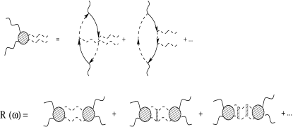
Figure 4: a) Diagrammatic representation of the Raman vertex for the interaction between light and magnons. Solid wavy lines represent light, solid and dashed straight lines represent conduction and valence electrons, and dashed wavy lines represent magnons. There are other diagrams (not shown) whose role is to cancel parasitic contributions from these two diagrams cf . b) Diagrammatic derivation of Eq. (2). Shaded rectangles represent $V(k,l)$.

The last element required for the computation of two-magnon Raman scattering is the magnon-magnon interaction. To derive it, we note that at large $U$, the magnetic properties of the Hubbard model are adequately described by the effective Heisenberg Hamiltonian $H=\sum_{r,\mu}\left(J_{1}{\bf S}_{r}{\bf S}_{r+\mu_{x}}+J_{2}{\bf S}_{r}{\bf S}_{r+\mu_{y}}\right)$. Applying the Holstein-Primakoff transformation to this Hamiltonian, and diagonalizing the quadratic form, we reproduce the magnon dispersion and also obtain the four-magnon interaction vertex. In the quasiclassical approximation, only the term $H_{int}=-V(k,l)e^{\dagger}_{k}e^{\dagger}_{-k}e_{l}e_{-l}$ with two creation and two annihilation boson operators $e$ is relevant cf . For $V(k,l)$, we obtained

$$V(k,l)=\frac{1}{4}\left[J_{2}+J_{1}(\cos(k-l)+\cos(k+l))\right](\mu_{k}^{2}\mu_{l}^{2}$$

$$+\lambda_{k}^{2}\lambda_{l}^{2})+\left[J_{2}+J_{1}(1+\cos(k-l))\right]\mu_{k}\mu_{l}\lambda_{k}\lambda_{l}$$

$$-\frac{1}{4}\left[3J_{2}/2+J_{1}(\cos(k)+2\cos(l))\right]\mu_{k}\lambda_{k}\left(\mu_{l}^{2}+\lambda_{l}^{2}\right)$$

$$-\frac{1}{4}\left[3J_{2}/2+J_{1}(\cos(l)+2\cos(k))\right]\mu_{l}\lambda_{l}\left(\mu_{k}^{2}+\lambda_{k}^{2}\right).$$ (6)

The coherence factors $\mu_{k}$ and $\lambda_{k}$ are given by

$$\mu_{k} = \frac{1}{\sqrt{2}}\sqrt{\frac{2J_{1}S+J_{2}S}{\epsilon(k)}+1},$$

$$\lambda_{k} = \frac{1}{\sqrt{2}}\frac{2J_{1}S\cos(k)+J_{2}S}{\left|2J_{1}S\cos(k)+J_{2}S\right|}\sqrt{\frac{2J_{1}S+J_{2}S}{\epsilon(k)}-1}.$$ (7)

With these results at hand, we can now compute the Raman intensity $R(\omega)$. Without magnon-magnon interaction, the Raman intensity $R(\omega)=-ImR_{0}(\omega)$, where

$$R_{0}(\omega)=\frac{i}{2\pi}\sum_{k}\int d\omega^{\prime}M^{2}_{R}(k)G_{k,\omega^{\prime}}G_{-k,\omega-\omega^{\prime}},$$ (8)

and $G_{k,\omega}=1/(\omega-\epsilon(k)+i\delta{\text{s}gn}\omega)$ is a magnon propagator. Substituting the result for $M_{R}(k)$ from (5) and evaluating the integral over $\omega^{\prime}$, we obtain

$$R_{0}(\omega)=(2J_{1}J_{2}S)^{2}\sum_{k}\left[\frac{1-\cos(k)}{\epsilon(k)}\right]^{2}~{}\frac{1}{\omega-2\epsilon(k)+i\delta}.$$ (9)

Like we said, the magnon dispersion $\epsilon(k)$, Eq. (1), has a maximum $\epsilon_{max}=2J_{1}S(1+J_{2}/2J_{1})$ at $k=k_{0}=\arccos(-J_{2}/(2J_{1}))$, and a minimum $\epsilon_{min}=S\sqrt{8J_{1}J_{2}}$ at $k=\pi$. Near the maximum and the minimum of $\epsilon(k)$, the magnon density of states $N(\epsilon)=dk/d\epsilon(k)$ diverges as a square-root of a distance to either $\epsilon_{min}$ or $\epsilon_{max}$. Replacing $\int dk$ by $\int N(\epsilon)d\epsilon$, we reproduce Eq. (3). Below $2\epsilon_{min}$, $R_{0}(\omega)$ is finite because of low-energy magnon states at small $k$, but is reduced due to the factor $[(1-\cos k)/\epsilon(k)]^{2}\propto k^{2}$. We found from (9) that as $\omega$ approaches $2\epsilon_{min}$ from below, $ImR_{0}(\omega)$ tends to constant value. It then jumps to infinity at $\omega=2\epsilon_{min}+0$, and decays as $1/\sqrt{\omega-2\epsilon_{min}}$ at larger frequencies(see Fig. 2).

When magnon-magnon interaction is included, the full $R(\omega)$ is given by Eq. (2), where $a=V(k,l)/(M_{R}(k)M_{R}(l))^{1/2}$ (see Fig. 4b). Near the two points where the density of states diverges, the interaction $V(k,l)$ from (6), (7) can be approximated by $V(\pi,\pi)=(J_{1}+J_{2}/2)/2$, and $V(k_{0},k_{0})=J_{2}(1+J_{2}/2J_{1})/4$. Using these forms, we obtain, e.g., near $2\epsilon_{min}$:

$$R(\omega)\propto Im\left[\frac{I(\omega)}{1+2V(\pi,\pi)~{}I(\omega)}\right],~{}I(\omega)=\sum_{k\approx\pi}\frac{1}{\omega-2\epsilon(k)}.$$ (10)

and $\omega=\omega+i\delta$. Comparing (9) and (10), we see that there are two differences between $R_{0}(\omega)=-ImR_{0}(\omega)\propto-ImI(\omega)$ and $R(\omega)$. First, $R(\omega)$ vanishes at $2\epsilon_{min}$ because the divergence in $ImI(\omega)$ in the numerator of (10) is overcompensated by even stronger divergence in the denominator. By the same reason, $R(\omega)$ also vanishes at $2\epsilon_{max}$ (and at $2\epsilon_{0}$ at finite $S$). Second, below $2\epsilon_{min}$, $ImI(\omega)$ is small and $ReI(\omega)$ is negative and behaves as $-1/\sqrt{2\epsilon_{min}-\omega}$. Then, at some $\omega=\omega_{res}<2\epsilon_{min}$, $2V(\pi,\pi)ReI(\omega_{res})=0$, and $R(\omega)$ develops a pseudo-resonance. Near $2\epsilon_{max}$, $ReI(\omega)$ is positive, and the resonance does not develop.

In Fig. 3a we plot $R(\omega)$ obtained by solving Eq. (2) numerically using Eqs. (6) and (7) for magnon-magnon interaction, and Eq. (5) for the Raman vertex, and by formally extending the quasiclassical formulas to $S=1/2$. We see that $R(\omega)$ has a sharp peak slightly below $2\epsilon_{min}$. The position of the peak and its width somewhat depend on the ratio $J_{2}/J_{1}$, but for not very small $J_{2}/J_{1}$ this dependence is rather moderate. For $J_{2}=0.5J_{1}$, the peak is located near $2J_{1}$, and its FWHM is $0.4J_{1}$. In between $2\epsilon_{min}$ and $2\epsilon_{max}$, the intensity passes through a maximum, but $R(\omega)$ at the maximum is much smaller than at the peak below $2\epsilon_{min}$. Like we said, for $S=1/2$, numerical results indicate uhrig ; uhrig_2 that the peak is more broad then in the quasiclassical analysis extended to $S=1/2$. For larger $S$, however, the quasiclassical results should be more accurate.

To conclude, in this paper we argued that the Raman intensity in spin $S$ two-leg spin-ladder materials has a pseudo-resonance peak. The peak originates from the existence of a local minimum in the magnon excitation spectrum, and is located slightly below twice the magnon energy at the minimum. The physics leading to the peak is similar to the excitonic scenario for the neutron and Raman resonances in the superconducting state of the cuprates. At large $S$, the peak is quite narrow, its intrinsic width scales as $1/S$. For $S=1/2$, though, the pseudo-resonance may be already rather broad.

We thank G. Blumberg and G. S. Uhrig for useful discussions and critical comments. The research was supported by NSF DMR 0240238 (A.V. Ch)

References

• (1) A. Gozar, G. Blumberg, B. S. Dennis, B. S. Shastry, M. Motoyama, H. Esaki, and S. Uchida, Phys. Rev. Lett. 87, 197202 (2001). For a review see A. Gozar and B. Blumberg, Collective Spin and Charge Excitaions in (Sr, La)14-xCaxCu24O41 Quantum Spin Ladders.
• (2) S. Sugai and M. Suzuki, Phys. Status Solidi B 215, 653 (1999).
• (3) A. Gossling, U. Kuhlmann, C. Thomsen, A. Loffert, C. Gross, and W. Assmus, Phys. Rev. B 67, 052403 (2003).
• (4) C. Knetter, K. P. Schmidt, M. Gruninger, and G. S. Uhrig, Phys. Rev. Lett.87, 167204 (2001).
• (5) S. Trebst, H. Monien, C. J. Hamer, W.H. Zheng, R. R. P. Singh, Phys. Rev. Lett. 85, 4373 (2000); V. N. Kotov, O. P. Sushkov, and R. Eder, Phys. Rev. B 59, 6266 (1999).
• (6) K. P. Schmidt, C. Knetter, and G. S. Uhrig, Europhys. Lett. 56, 877 (2001);K. P. Schmidt, C. Knetter, M Gruninger, and G. S. Uhrig, Phys. Rev. Lett. 90, 167201 (2003).
• (7) P. J. Freitas and R. R. P. Singh, Phys. Rev. B 62, 14113 (2000).
• (8) see, e.g., A. V. Chubukov and M.R. Norman, Phys. Rev. B 70, 174505 (2004) and references therein.
• (9) A. V. Chubukov, D. K. Morr and G. Blumberg, Solid State Commun., 112, 183 (1999); A. V. Chubukov, T. Devereaux, and M. Klein, in preparation. For experimental work, see G. Blumberg et al, Science 278, 1427 (1997); J. Phys. Chem. Solids 59, 1932 (1998).
• (10) R.R.P. Singh, Comments Condens. Matter Physics 15, 241 (1991).
• (11) A. V. Chubukov and D. M. Frenkel, Phys. Rev. B 52, 9760 (1995); F. Schonfeld, A. P. Kampf, and E. Muller-Hatrmann, Z. Phys. B 102, 25 (1997).
• (12) F. D. M. Haldane, Phys. Lett. 93A, 464 (1983).
• (13) The validity of the large $U$ approach for $Sr_{14}Cu_{24}O_{41}$ has been questioned in recent studiesΒ FreitasSingh .
• (14) J.B. Parkinson, J. Phys. C 2, 2012 (1969); R. J. Elliott and M. F. Thorpe, ibid 2, 1630 (1969).
• (15) H. F. Fong, P. Bourges, Y. Sidis, L. P. Regnault, J. Bossy, A. Ivanov, D. L. Milius, I. A. Aksay, and B. Keimer, Phys. Rev. B 61, 14773 (2000) and references within.
• (16) J. R. Schrieffer, X. G. Wen, and S. C. Zhang, Phys. Rev. B, 39, 11663 (1989); A. V. Chubukov and D. M. Frenkel, Phys. Rev. B 46, 11884 (1992).
• (17) B. S. Shastry and B. I. Shraiman, Phys. Rev. Lett. 65, 1068 (1990); Intl. J. Mod. Phys. B 5, 365 (1991).
• (18) P. A. Fleury and R. Loudon, Phys. Rev. 166, 514 (1968).