Symbiosis in the Bak-Sneppen Model for Biological Evolution with Economic Applications

Abstract

In the present work we extend the Bak-Sneppen model for biological evolution by introducing local interactions between species. This “environmental” perturbation modifies the intrinsic fitness of each element of the ecology, leading to higher survival probability, even for the less fit. While the system still self-organizes toward a critical state, the distribution of fitness broadens, losing the classical step-function shape. A possible application in economics is discussed, where firms are represented like evolving species linked by mutual interests.

In the past two decades several studies have been devoted to the investigation of the ubiquitous presence of power laws in natural and social systems. An important contribution to this field of research has been given by Bak, Tang and Wiesenfeld (BTW) [1, 2], who developed the concept of self-organized criticality (SOC). The key idea behind SOC is that complex systems, that is systems constituted of many interacting elements, although obeying different microscopic physics, may exhibit similar dynamical behaviour, statistically described by the appearance of power laws in the distributions of their characteristic features. The lack of a characteristic scale, indicated by the power laws, is equivalent to those of physical systems during a phase transition – that is at the critical point. It is worth emphasizing that the original idea [1, 2] was that the critical state is reached “naturally”, without any external tuning. This is the origin of the adjective self-organized. In reality a certain degree of tuning is necessary: implicit tunings like local conservation laws and specific boundary conditions seem to be important ingredients for the appearance of power laws [3].

The classical example of a system exhibiting SOC behaviour is the 2D sandpile model [1, 2, 3, 4]. Here the cells of a grid are randomly filled, by an external driver, with “sand”. When the gradient between two adjacent cells exceeds a certain threshold a redistribution of the sand occurs, leading to more instabilities and further redistributions. The avalanche dynamics that drives the system from one metastable state to another is the benchmark of all systems exhibiting SOC. In particular, the distribution of the avalanche sizes, their duration and the energy released, all obey power laws.

The framework of self-organized criticality has been claimed to play an important role in solar flaring [5, 6], space plasmas [7, 8] and earthquakes [9, 10, 11, 12, 13] in the context of both astrophysics and geophysics. In biology SOC has been linked to the punctuated equilibrium [12] in species evolution [14]. Some work has also been carried out in the social sciences. In particular, traffic flow and traffic jams [15, 16, 17, 18], wars [19], as well as stock-market [4, 20, 21, 22] dynamics, have been studied. A more detailed list of subjects and references related to SOC can be found in the review paper of Turcotte [4].

In the present work we extend the Bak-Sneppen (BS) model for evolution [14] by introducing explicit coupling terms in the fitness of each species of the ecology. We find that the equilibrium configuration of the model can be deeply influenced by the environmental forces, leading to a wider survival probability also for species with a lower degree of adaptation. A possible application of our extension of the BS model to the economic world is that the distribution of global-fitness can be related to the size distribution of firms in the most developed markets. In this respect the evolution of firms is seen as a punctuated equilibrium process in which the convolution of mutual interest can justify the spreading in size of the firms themselves.

The toy model proposed in 1993 by Bak and Sneppen [14] is one of the most popular models for biological evolution. The main idea behind this model is that each species can be uniquely characterized by a single parameter called fitness. The fitness of a species represents its degree of adaptation with respect to the external environment. Highly adapted species will hardly undergo any successful, spontaneous mutations. At the opposite end of the scale, if a species has a very low degree of fitness it needs to mutate in order to survive and its mutation automatically influences the other species belonging to the same environment. These concepts can be easily formulated as a simple 1D model. Suppose that the ecology can be represented by a periodic array of $N$ cells and each cell, $i$, is assigned a fitness, $B(i)$, taken from a uniform distribution between 0 and 1. Once we have fixed the initial condition, for each discrete time-step, the dynamical evolution of the system works as follows:

a) locate the species with minimum fitness – that is, the one most likely to mutate, $k$,

b) change the fitness of $k$ and that of its neighbours (species related) according to

$$B(k-1)\rightarrow u_{1},$$

$$B(k)\rightarrow u_{2},$$

$$B(k+1)\rightarrow u_{3},$$ (1)

where the new fitness value, $u_{i}$, is a random number taken from a uniform distribution bounded between 0 and 1.

From numerical [14] and analytical [23] studies it has been shown that the values of the fitness evolve to a step function, in the thermodynamic limit ($N\rightarrow\infty$), characterized by a single value, $B_{c}$. For $B<B_{c}$ the distribution of fitness, $P(B)$, is uniformly equal to zero while for $B>B_{c}$ we have $P(B)=1/(1-B_{c})$, determined by the normalization condition. An example is shown in Fig. 1 (a) and (b).

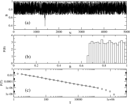
Figure 1: (a): Snapshot of the fitness, $B$, after $8\cdot 10^{7}$ time steps in a stable configuration. All the barriers are above a critical threshold, except for those around 1500, where an avalanche is clearly visible. (b): Probability distribution of the barriers, $P(B)$, shown in (a). While the distribution is equal to zero on the left hand side, a plateau is evident for $B>B_{c}\sim 0.667$. In the thermodynamic limit the plateau will become exactly a constant. In this case the simulation has been carried out for $N=5000$ species. (c): Probability distribution, $P(T)$, of avalanche duration, $T$, in the stationary regime for the Bak-Sneppen model. The avalanche time series has been recorded in the stationary state of the system, after $\sim 10^{7}$ iterations for $N=2000$ species. The power law exponent is $\gamma\sim 1$.

In this model it is also possible to define a bust-like avalanche dynamics. Suppose we fix a threshold for the fitness, $B_{0}$ and consider $B_{m}(t)$ as the minimal fitness at time step $t$. If at a certain time step, $t_{1}$, it happens that $B_{m}(t_{1})<B_{0}$ then we can measure the interval of time, $T$, needed for having again $B_{m}(t_{1}+T)>B_{0}$. In this case an avalanche of duration, or size, $T$ has taken place in order to restore a minimal fitness in the system. If $B_{0}=B_{c}$ then we have $P(T)\sim T^{-\gamma}$: the system is critical, see Fig. 1(c).

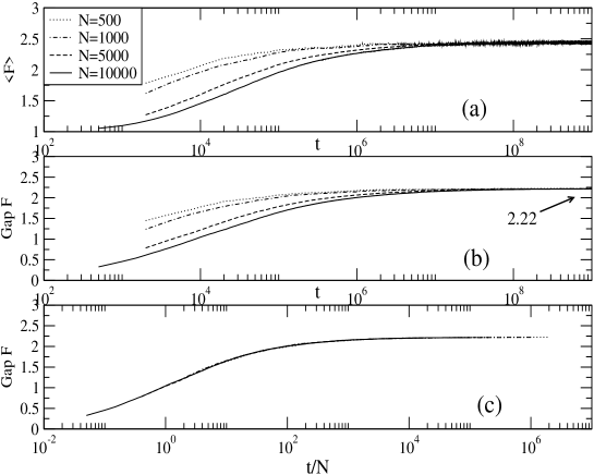
Figure 2: Average value (a), $\langle\dots\rangle$, and gap (b), Gap, function for the global fitness $F$ and different system size for simulations up to $10^{9}$ mutations, $t$. Note that the gap function converges approximately to the value $F_{c}\sim 2.22$ that corresponds to the critical threshold for this model. A simple rescaling of the time, $t\rightarrow t/N$, brings the curves to collapse into a single one, as shown in (c).

According to this model the great mass extinctions of species, like dinosaurs for example, can be explained in terms of burst-like dynamics. A small perturbation in an critical self-connected system can trigger a chain reaction that may influence a great part of the species in the ecosystem. Time series of fossils samples seem to be in agreement with this avalanche dynamics in the extinction/evolution of species. A more detailed discussion of the BS model goes beyond the scope of the present work. For a general review see Ref. [24].

Despite its simplicity, the BS model evolves according to a complex dynamics and it is able to explain some empirical features of the biological evolution [14]. An implicit assumption in the model is that every species is deeply connected to its environment. A mutation on a single element automatically triggers a mutation in its neighbors.

But is this approximation always appropriate? Consider for example three species in a one dimensional array and suppose that $B_{i}=B_{min}$ while $B_{i-1}\cong B_{i+1}\cong 1$. In the standard BS model the $i$th cell undergoes to mutation that also triggers a change in $B_{i-1}$ and $B_{i+1}$. From a biological point of view it means that two extremely well adapted species have to mutate in order to cope with the mutation of the $i$th species. This can be interpreted as a very particular (pessimistic) case – such as, for example, the case where the $i$th species is the main source of food for both the other species.

In order to stress this idea we use some examples from different areas in which a similar evolutionary dynamics can be applied. Suppose that a new unfit or unskilled player joins a strong team. Will this player trigger a regression in the team performance or will the team compensate for this lack of skills? This is a small perturbation after all.

Another example comes from economics. In this case, it has been shown [25, 26, 27], that the dynamics of different firms is correlated. In fact, it is not unusual for a company to own large amounts of stock of other companies and so on. The result is an entangled environment, where the evolution of a firm is, in a way, linked to the evolution of its network of interaction. Is it then possible, in this case, for an wealthy environment to sustain an unfit element, or will its lack of “fitness” bring to the brink of the financial collapse all the other partners, as the BS model would suggest?

We provide an answer to these questions using a modified version of the BS model that takes into account the feedback of the environment on the single element. We refer to this model incorporating Local Interactions in the BS model as the LIBS model. For the sake of simplicity we do not consider the topology of the interaction, that may be very complex; rather, we use a simple 1D array. The influence of the network structure on the dynamics of the model will be discussed in our future work.

As a first approximation we consider our species to be arranged on a one dimensional array with nearest neighbor interactions. This means that the micro-environment is composed of three cells. The value of the fitness, $B$, for each cell is taken, according to the BS model, from a uniform distribution between zero and one. The fitness parameter, $B_{i}$, of the $i$th cell represents the self-fitness of the species. Motivated by the aforementioned examples, we add an environmental contribution to the self-fitness that leads to a global-fitness, $F_{i}$, according to

$$F_{i}=B_{i}+\Lambda_{i,i-1}B_{i-1}+\Lambda_{i,i+1}B_{i+1},$$ (2)

where $\Lambda_{i,i-1}$ and $\Lambda_{i,i+1}$ are the fractions of fitness that the $i$th cell shares with its neighbours. The matrix of $\Lambda$s is not symmetric, reflecting the fact that the contribution in one direction can be very different that the contribution in the other. This is equivalent to considering a directed weighted graph with a trivial necklace topology.

In the sport example, the global fitness corresponds to the fit players that contribute to sustaining the unskilled team-mate. From the economic point of view it represents the capability of a firm to gain benefits from its partnerships with other firms. In this particular case, $B_{i}$ represents the wealth generated by the firm itself, while the other two terms represent the contribution, in different forms, from the linked firms. In general, we can consider the new terms in the definition of $F_{i}$ as short ranged random forces acting on the $i$th cell.

At the beginning of the simulation the self-fitness is drawn from a uniform distribution between zero and one. The same is done for the link weights, $\Lambda_{ij}$. It is worth emphasizing that, in general, for two cells $i$ and $j$, $\Lambda_{ij}\neq\Lambda_{ji}$.

Assuming that the neighbours can cooperate in defining the fitness of a species (optimistic view), the extremal dynamics is moved from $B_{min}$ to $F_{min}$. Once the site with minimum global fitness, $k$, is located, then the self-fitness and the interactions of this species are redrawn according to the following rules:

$$\Lambda_{k,k-1}\rightarrow u_{1},$$

$$\Lambda_{k-1,k}\rightarrow u_{2},$$

$$B(k)\rightarrow u_{3},$$

$$\Lambda_{k,k+1}\rightarrow u_{4},$$

$$\Lambda_{k+1,k}\rightarrow u_{5},$$ (3)

where the new values for the changed quantities are taken from a uniform distribution between zero and one, as in the BS model. However, in contrast to the BS model, a change in the fitness of the $k$th species does not automatically trigger a change in the neighbours. Only the interactions are changed.

In order to test the stability of the model we monitor the average fitness and the gap function, $G(t)$, for both $B$ and $F$. The gap function is nothing but the tracking function of the minimum of $B_{min}(t)$ ( or $F_{min}(t)$). At $t=0$ we have $G(0)=B_{min}(0)$ ( or $G(0)=F_{min}(0)$). As the evolution proceeds eventually for a certain $t_{1}$ we will have $B_{min}(t_{1})>B_{min}(0)$ ( or $F_{min}(t_{1})>F_{min}(0)$) as the minimum barriers are converging toward the critical value. The gap function is then updated as $G(t_{1})=B_{min}(t_{1})$ ( or $G(t_{1})=F_{min}(t_{1})$) and so on. It is easy to see that in the stationary state the gap function converges toward the critical value .

In Fig. 2 the time series of average values and the gap function of $F$ are plotted for different number of species in the ecology. The time to reach the stable state depends strongly on the size: for $N=10^{4}$, the largest system in our simulations, we need approximately $t\sim 10^{8}$ mutations to achieve the equilibrium. Note also that a simple rescaling, $t\rightarrow t/N$, leads to a collapse of these curves. The relaxation times in the BS model are, approximately, one order of magnitude lower compared to the LIBS model of the same size (or in rescaled time).

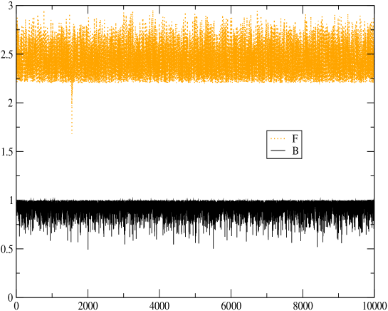
Figure 3: Snapshot of the grid, $N=10^{4}$, in a stable configuration for fitness $B$ and global fitness $F$.

A snapshot of the grid in the stable configuration is shown in Fig. 3. We notice immediately that that the local fitness is no longer distributed like a step function (as for BS). Rather a long, exponential, tail of low fitness is evident, as shown in Fig. 4 (Left). The cells with a higher local fitness still have a greater probability to survive but the global-fitness, or the presence of environmental partnerships, widens the possibility of survival, even for some species with a lower degree of self-fitness.

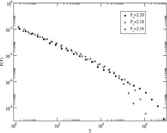
Figure 5: Probability distribution, $P(T)$, of the avalanche duration, $T$, in the LIBS model. Three different thresholds during the stable regime are considered. The critical exponent is $\gamma\sim 0.83$. For $F_{c}=2.20$ we are very close to the critical point and very large avalanches are present.

If we examine the global-fitness, a single avalanche is present – as in the classical BS model. Moreover the probability distribution function for the avalanche duration, shown in Fig. 5 and computed with respect to $F$, is power law distributed, in relation with the criticality of the model. The index of the distribution turns out to be different from that of BS: the change in the dynamics has also led to a change in the universality class of the model.

The distribution of global-fitness, shown in Fig. 4 (Right), has a polynomial decay (4th order fit in the plot) above a critical threshold, as a result of the convolution of stochastic variables. A similar behaviour can be found also in the size distribution of firms, suggesting a possible practical application to the LIBS model. Axtell [30] analyzed the size distribution of U.S. companies, defined as the total number of employee, during 1997. He fund that it could be well represented by a Zipf distribution, $P(s)\sim s^{-\alpha}$ with $\alpha\sim 1$, being $s$ the size of the firm. This seemed to confirm the validity of the “Gibrat’s principle” according to which the firm growth rate is independent on its size. Further investigation on this issue has been carried on by Gaffeo et al. [31], which analyzed a database of companies for the G7 countries from 1987 to 2000. Their analysis could confirm the findings of Axtell, power law distribution with $\alpha\sim 1$, just for some particular definition of firm size, that is not unambiguous, and for some particular business periods. What they found, in general, is a robust power law behaviour, although the index could change with the time window analyzed and the definition of firm size, in contrast with the standard theory of Gibrat. The qualitative discrepancies between $P(F)$ and the distribution empirically found for the size distribution of firms can be explained if we take into account more complex topologies for interactions between species, or economical entities in this case. Different kinds of convolution can generate a different shape in the distribution of the global-fitness as it can be easily deduced by writing Eq. 2 in a general form as

$$F_{i}=\sum_{j=1}^{k_{i}}\Lambda_{i,j}B_{i,j},$$ (4)

where $\Lambda_{i,i}=1$ and the sum over $j$ is extended to all the $k_{i}$ neighbours of the $i$th species. In Eq. 4 no particular topology is specified. For an isotropic model on a $D$-dimensional lattice, $k_{i}$ is equal for all the species and depends just on $D$ and the definition of neighborhood: the theoretical boundaries for $F$ are equal for all the species and we can talk about a “democratic” model. However, recent studies have shown [32, 33] that, in real biological and social systems the number of links per elementary unit, $k$, is not constant, but characterized by a non-trivial probability distribution function, $P(k)$, as a result of the complex nature of the interactions between species or individuals. From Eq. 4, we can immediately see that, by adopting a complex network as underlying structure for the interaction between species, we move to a model in which each species have different boundary values for the global-fitness, since $0\leq F_{i}\leq k_{i}$. This inequality have a straightforward interpretation: species with a large number of connections will have an higher barrier against environmental changes due to the fact that they can relay on numerous resources. A simple way to obtain a complex network structure is by considering an open system, where the number of species is not fixed but grows in time, as for example the firms in a dynamic economy. In this case, it will be more likely for the new economic entities to be connected with a well established one that has already a large number of connections (growth and preferential attachment are actually the two main ingredients for the Albert-Barab$\acute{a}$si model for scale-free networks [32]). According to our model these “hubs”, that is companies such as General Motors or Coca Cola, have an higher chance of surviving a turbulent period compared to isolated nodes: they have a larger influence in the dynamics of the model. This simple consideration, although not exhaustive, show how the underling topology of the interactions can play an important role in the final distribution of the global fitness. Further analytical and numerical test would be of great importance in order to understand the dynamics of the LIBS model and to which extend it can be applied to real systems. It is also worth pointing out that another parameter related to $P(F)$ is the domain of $B$ itself, that, in the present, case we assume to be uniform in the interval (0,1). In fact, a change in this distribution, while preserving the dynamics of the model, would lead to a different shape in the final distribution of $F$. While these important issues will be addressed in our future work, in Appendix we report a further extension of the model where also the second-nearest neighbour interaction is considered.

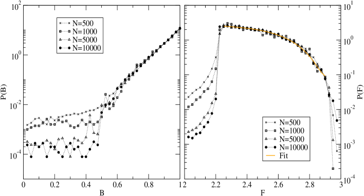
Figure 4: Left: probability distribution function, $P(B)$, for fitness $B$. The step distribution of the standard BS model has been replaced with an exponential distribution with a cut-off at $F\sim 0.55$. Right: Probability distribution, $P(F)$, for the global-fitness, $F$, and fit with a fourth order polynomial. In this case a sharp threshold is visible, as in the standard BS model, indicating that poor fitness environments undergo mutation. As we consider larger $N$ the transition, at $F_{c}\sim 2.22$, gets sharper and sharper as expected by a finite size analysis. The values of the $P(F)$ below this threshold are related to the recorded avalanches. The distributions shown in these plots are the results of an average over 50 different configurations in the stable regime.

The results obtained with the LIBS model confirm the relevance of self-organized criticality in complex systems and, in particular, economics. The concept of mutual cooperation, introduced via the global-fitness, can explain the ubiquity of broad tails in the distribution of characteristic quantities of physical and social systems in terms of a convolution of variables between elements of the network of interaction. In the economic context, this asymptotic behaviour can be related to the empirical findings concerning the distribution of the size of firms. The possible relevance of self-organized criticality in economics has already been suggested by recent theoretical and empirical studies [20, 21, 35, 36], while possible applications of the BS model in this field can be found in Refs. [37, 38, 39]. The application of the SOC concept to social sciences can, in general, be motivated by empirical observations of the “intermittent” activity in the human dynamics at every level, from wars to revolutions and, in particular, intellectual production where moments of frenetic activity can be alternated by long breaks, which length cannot be predicted (this holds, indeed, for one of the authors, M.B.). This process is, in a way, similar to the discharge, via avalanches, needed in the classical sandpile model, to restore the critical slope. In a real economic world a wide series of changes, similar to avalanches, can be triggered by exogenous or endogenous shocks related to structural changes at macroeconomic level, for example the creation and successive enlargement of the European community or the fall of the Soviet empire, or at microeconomic level, as the invention of a new technology [40]. Since the shocks leading to avalanches are of different nature, we also expect the existence of different time scales involved in the self-organization process. In SOC systems, in general, the existence of a sharp separation between time scales, energy storage and relaxation, appears to be a strict prerequisite. In the BS model, as in the LIBS model, by mutating one unit at the time, we implicitly assume that the time to extinction, $t_{e}$, of a species depends exponentially on its global fitness, that is $t_{e}(i)\propto e^{F_{i}}$. The exponential separation of the extinction times is at the core of the “punctuation”. In economics terms we can still assume this behaviour: changes of poorly fitted firms can be simply related to small microeconomic fluctuations that can happen in time scales of the order of weeks or months while much longer times are needed to change the fitness of an highly adapted company. In the latter case radical changes are needed, as for example a switch from a political regime to another, that may take centuries to happen.

In conclusion, we have extended the Bak-Sneppen model for biological evolution by introducing explicitly local interactions between elements of the ecology. Numerical simulations have shown how the dynamics of the model, while still leading to a self-organized critical state, can be largely effected by the environmental forces, leading to smoother distributions in both the intrinsic fitness, $B$, and the global fitness, $F$. As already pointed out by Grassberger [41] the BS model cannot be taken too seriously for describing the punctuated equilibrium of biological evolution. Nevertheless, because of its simplicity, it can easily be used as paradigm for other complex systems. In the present work we suggest a possible application of our extension of the BS model to the economic world. In particular the distribution of global-fitness can be related to the size distribution of firms in the most developed markets. In this respect the evolution of firms is seen as a punctuated equilibrium process in which the convolution of mutual interest can justify the spreading in size of the firms themselves. It is worth pointing out that the actual shape of the distribution of global-fitness is related to the topology of the interaction. A simple 1D model cannot be expected to account completely for the power law distribution observed in the size of firms. Future work will be devoted to the application of the model proposed in this paper to more complex topologies – as, for example, to scale-free networks [32, 33], that are more likely to reproduce the real interactions between economic entities.

Appendix

We consider now a further extension of the LIBS model by including the second nearest neighbours interactions in the simple one dimensional topology. The global-fitness of Eq. 2 becomes

$$F_{i}=B_{i}+\Lambda_{i,i-1}B_{i-1}+\Lambda_{i,i+1}B_{i+1}+\Lambda_{i,i-2}B_{i-2}+\Lambda_{i,i+2}B_{i+2},$$ (5)

where we the second order coefficients are not independent random numbers but $\Lambda_{i,i\pm 2}=\Lambda_{i,i\pm 1}\cdot\Lambda_{i\pm 1,i\pm 2}$. The reason behind this choice, that can be easily extended to the $n$th order neighbours, is motivated by the assumption that the higher order interactions are damped by the “distance” between the two species and therefore $\Lambda_{i,i\pm 2}\leq\Lambda_{i,i\pm 1}$. By using this formulation, we attempt to mimic a hierarchical dependence of the global fitness in the ecology: species become explicitly related to their second nearest neighbours via the mediation of their first neighbours and so on. Using these constrains the mutation rules remain the same as in Eq. 3 since a change in the first order coefficients triggers automatically a change also in the higher order ones.

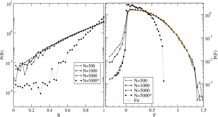
Figure 6: Left: distribution of self-fitness, $B$, for the second order neighbours and different grid size, $N$. The distribution for the first order neighbours is also plotted (*). Note that an extension of the neighborhood leads to a slower decay rate. Moreover, a clear cut-off for low $B$ is not evident anymore. Right: distribution of global fitness $F$. In this case the distributions have been rescaled according to $F\rightarrow F-F_{c}$. For the second order neighbours we have $F_{c}\sim 2.37$. The fit with a sixth order polynomial, also shown, produces a smaller $\chi^{2}$ compared to the fourth order used for the first nearest neighbour case.

The dynamics that results from the numerical simulations is similar to the first neighbours LIBS model: after an extensive transient we reach a critical stationary state characterized by avalanches of mutations, which size, $T$, is power law distributed. The distributions for $B$ and $F$, in the stable regime, are shown in Fig. 6 along with the distribution obtained by considering just the first neighbour interaction. In the case of $B$ we can notice that by enlarging the neighborhood the distribution show a slower decaying rate and they appear to be smoother. In this case we have an exponential decay all the way down to zero, without any clear cut-off for low $B$. Despite their fitness, all the species have a chance of survival if sustained by an healthy environment. Regarding the global fitness, instead, a polynomial decay is still evident, although the order is higher compared to the first neighbours case. In is also important to notice that a relative large change in the theoretical range for $F$, which bounds are now $0\leq F_{i}\leq 5$, does not lead to a consequent rise in the threshold value that moves just slightly from $F_{c}\sim 2.22$ to $F_{c}\sim 2.37$. This is equivalent to say that, in the previous case, in order to be considered “fit”, a species has to exceed the $\sim$ 74% of the possible range for $F$, now the $\sim$ 48% is sufficient! In conclusion, a hierarchical extension of the cooperation between species in the LIBS model leads to an easier adaptation and survival probability: the more compact the ecosystem is the higher will be the chances of survival of each single species as long as they cooperate for their mutual interest.

References

- [1] Bak, P., Tang, C. & Wiesenfeld, K. Self-organized criticality: an explanation of 1/f noise. Phys. Rev. Lett. 59, 381 (1987).
- [2] Bak, P., Tang, C. & Wiesenfeld, K. Self-organized criticality. Phys. Rev. A 38, 364 (1988).
- [3] Jensen, H.J., Self-Organized Criticality: Emergent Complex Behavior in Physical and Biological Systems, (Cambridge University Press, Cambridge, 1998).
- [4] Turcotte, D. L. Self-organized criticality. Rep. Prog. Phys. 62, 1377 (1999).
- [5] Lu, E.T. & Hamilton, R.J. Avalanches and the distribution of solar flares. Astrophys.J. 380, L89 (1991).
- [6] Lu, E.T., Hamilton, R.J., McTieran, J.M., Bromund, K.R. Solar flares and avalanches in driven dissipative systems. Astrophys.J. 412, 841 (1993).
- [7] Chang, T., et al., Advances in Space Environmental Research, Vol.I, (Kluwer Academic Publisher, AH Dordrecht, The Netherlands, 2003).
- [8] Valdiva, A., et al., Advances in Space Environmental Research, Vol.I, (Kluwer Academic Publisher, AH Dordrecht, The Netherlands, 2003).
- [9] Bak, P. & Tang, C. Earthquakes as a self-organized critical phenomenon. J. Geophys. Res. 94, 15 635 (1989).
- [10] Sornette A. & Sornette, D. Self-organized criticality and earthquakes Europhys. Lett. 9, 197 (1989).
- [11] Sornette, D., Davy, P., Sornette, A. Structuration of the lithosphere in plate tectonics as a self-organized critical phenomenon. J. Geophys. Res. 95, 17353 (1990).
- [12] Gould, S.J. & Eldredge, N. Punctuated equilibrium comes of age. Nature 366, 223 (1993).
- [13] Huang, J., Sauler, H., Sammis, C. & Sornette D. Precursors, aftershocks, criticality and self-organized criticality. Europhys. Lett. 41, 43 (1998).
- [14] Bak, P. & Sneppen, K. Punctuated equilibrium and criticality in a simple model of evolution Phys. Rev. Lett. 71, 4083 (1993).
- [15] Nagel, K. & Herrmann, H.J. Deterministic models for traffic jams. Physica A 199, 254 (1993).
- [16] Nagel, K., & Paczuski, M. Emergent traffic jams. Phys. Rev. E 51, 2909 (1995).
- [17] Nagatani, T. Self-organized criticality in 1D traffic flow model with inflow or outflow. J.Phys. A:Math.Gen. 28, L119 (1995).
- [18] Nagatani, T. Self-organized criticality in 1D traffic flow. Fractals 4, 279 (1996).
- [19] Roberts, D.C., & Turcotte, D.L. Fractality and self-organised criticality of wars Fractals 6, 351 (1998).
- [20] Bak, P., Chen, K., Scheinkman, J. & Woodford, M. Aggregate fluctuations from independent sectoral shocks: self-organized criticality in a model of production and inventory dynamics. Ric. Econ. 47, 3 (1993).
- [21] Bak, P., Paczuski, M. & Shubik, M. Price variations in a stock market with many agents. Physica A 246, 430 (1997).
- [22] Feigenbaum, J. Financial Physics. Rep. Prog. Phys. 66, 1611 (2003).
- [23] Flyvbjerg, H., Bak, P. & Sneppen, K. Mean field theory for a simple model of evolution. Phys. Rev. Lett. 71, 4087 (1993).
- [24] Paczuski, M., Maslov, S., & Bak, P. Avalanche dynamics in evolution, growth and depinning models. Phys. Rev. E 53, 414 (1996).
- [25] Vanderwalle, N., Brisbois, F. & Tordoir, X. Non-random topology of stock markets. Quant. Finance 1, 372 (2001).
- [26] Bonanno, G., Caldarelli, G., Lillo, F., Mantegna, R. N. Topology of correlation-based minimal spanning trees in real and model markets. Phys. Rev. E 68 , 46130 (2003).
- [27] Souma, W., Fujiwara, Y. & Aoyama, H. 9th Workshop on economics and heterogeneous interacting agents (WEHIA2004) May 27-29, 2004 at Kyoto University, Kyoto, Japan. Preprint: physics/0502005.
- [28] Tabelow, K. Gap function in finite Bak-Sneppen model Phys. Rev. E 63, 047101 (2001).
- [29] Head, D.A. Universal persistence exponents in an extremally driven system Phys. Rev. E 65, 027104 (2002).
- [30] Axtell, R.L. Zipf distribution of U.S. firm size Nature 293, 1818 (2001).
- [31] Gaffeo, E., Gallegati, M. & Palestrini, A. On the size distribution of firms: additional evidence from the G7 countries. Physica A 324, 117 (2003).
- [32] Albert, R. & Barabsi, A.-L. Statistical mechanics of complex networks. Rev. Mod. Phys. 74, 47 (2002).
- [33] Dorogovtsev, S.N. and Mendes, J.F.F., Evolution of networks. Adv. Phys. 51, 1079 (2001).
- [34] Mezard M., G. Parisi and Virasoro M. A., Spin Glass Theory and Beyond, (World Scientific, Singapore, 1987).
- [35] Ponzi, A. & Aizawa, Y. Criticality and punctuated equilibrium in spin system model of financial market. Chaos, Solitons & Fractals 11, 1739 (2000).
- [36] Bartolozzi, M., Leinweber, D.B. & Thomas, A.W. Self-organized criticality and stock market dynamics: an empirical study. Physica A 350, 451 (2005).
- [37] Cuniberti, G., Valleriani, A. & Vega, J.L. Effects of regulation on a self-organized market. Quant. Finance 1, 332 (2001).
- [38] Yamano, T. Regulation effects on market with Bak-Sneppen Model in high dimensions. Int. J. Mod. Phys. C 9, 1329 (2001).
- [39] Ausloos, M., Clippe, M. & Pekalski, A. Evolution of economic entities under heterogeneous political/environmental conditions within a Bak-Sneppen-like dynamics. Physica A 332, 394 (2004).
- [40] Day, R.H. The Divergent Dynamics of Economic Growth, (Cambridge University Press, Cambridge, 2004).
- [41] Grassberger, P. The Bak-Sneppen model for punctuated equilibrium. Phys. Lett. A 200, 277 (1995).