Energy diffusion in frustrated quantum spin chains exhibiting Gaussian orthogonal ensemble level statistics

Abstract

Frustrated quantum $XXZ$ spin chains with the next-nearest-neighbor (NNN) couplings are typically deterministic many-body systems exhibiting Gaussian orthogonal ensemble (GOE) spectral statistics. We investigate energy diffusion for these spin chains in the presence of a periodically oscillating magnetic field. Diffusion coefficients are found to obey the power law with respect to both the field strength and driving frequency with its power varying depending on the linear response and non-perturbative regimes. The widths of the linear response and the non-perturbative regimes depend on the strength of frustrations. We have also elucidated a mechanism for oscillation of energy diffusion in the case of weakened frustrations.

I Introduction

There exists an accumulation of studies on quantum dynamics of classically chaotic systems , e.g., kicked rotators, kicked spin-tops, hydrogen atoms in time-dependent electric field, and the standard map model, to mention a few. NS2001 Quantum suppression of energy diffusion, dynamical localization and other signatures of quantum chaos are notable in these dynamics. However, most of the systems treated so far are confined to those with a few degrees-of-freedom, and little attention is paid to dynamics of quantum many-body systemsJona ; Prosen ; Flambaum whose adiabatic energy levels are characterized by Gaussian orthogonal ensemble (GOE) spectral statistics, i.e., by a hallmark of quantum chaos. While some important contributions Wilkinson88 ; WilAus92 ; WilAus95 ; Bulgac ; Cohen00D ; Cohen00M ; Machida are devoted to dynamics of a kind of many-body systems, those systems are actually described by the random-matrix models, and not by deterministic quantum Hamiltonians. It is highly desirable to explore dynamical behaviors of deterministic quantum many-body systems exhibiting GOE or GUE spectral statistics.

On the other hand, the frustrated quantum spin systems have been receiving a wide attention, and we can find their realization in $s=\frac{1}{2}$ antiferromagnetic chains Cu(ampy)Br₂ Kikuchi and (N₂H₅)CuCl₃, Hagiwara and in $s=\frac{1}{2}$ triangular antiferromagnets. KPL The high-lying states of these quantum many-body systems deserve being studied in the context of ”quantum chaos.” The advantage of the frustrated quantum systems is that one can expect quantum chaotic behaviors appearing already in the low energy region near the ground state. Nakamura85 ; Yamasaki04 From the viewpoint of real physics of condensed matters, novel features observed in the low-energy region are very important and welcome. Recalling that in most of deterministic Hamiltonian systems quantum chaotic behaviors appear in high-lying states, the role of frustration is essential in the study of quantum dynamics from the ground state of deterministic many-body systems with GOE or Gaussian unitary ensemble (GUE) level statistics.

In this paper, we investigate dynamics of $XXZ$ quantum spin chains which have antiferromagnetic exchange interactions for the nearest-neighbor (NN) and the next-nearest-neighbor (NNN) couplings. The NNN couplings cause the frustration, i.e., difficulty in achieving the ground state, thereby attributing a name of frustrated quantum spin chains to these systems. In fact, the level statistics of the NNN coupled $XXZ$ spin chains without an applied magnetic field has been studied intensively in Refs. Kudo03, ; Kudo04, , and it has been shown that GOE behavior, which is typical of quantum chaos, appears already in the low energy region near the ground state. note ; note1 The ground-state phase diagram is shown in Ref. Nomura, for the NNN coupled $XXZ$ spin chains without a magnetic field.

A natural extension of the research is to investigate dynamics of the frustrated quantum spin chains with an applied periodically oscillating magnetic field. We calculate a time evolution of the system starting from their ground state and analyze the nature of energy diffusion. We shall numerically exhibit the time dependence of energy variance, and show how the diffusion coefficients depend on the coupling constants, the anisotropy parameters, the magnetic field and the frequency of the field. Furthermore, to compare with the energy diffusion in the case of weakened frustrations, we also investigate dynamics of the corresponding energy diffusion in $XXZ$ spin chains with small NNN couplings.

The organization of the paper is as follows: In Sec. II, we briefly describe a numerical approach to obtain the time evolution operator. In Sec. III we shall show the time dependence of energy variance starting from the ground state of the many-body system and explain a way to evaluate diffusion coefficients. Section IV elucidates how diffusion coefficients depend on field strength and driving frequency. Here power laws are shown to exist in the linear response and non-perturbative regions. Section V is devoted to a mechanism of oscillation of energy diffusion. Conclusions are given in Sec. VI.

II Numerical Procedure

We give Hamiltonian for the NN and NNN exchange-coupled spin chain on $L$ sites with a time-periodic oscillating magnetic field as

$$\mathcal{H}(t)=\mathcal{H}_{0}+\mathcal{H}_{1}(t),$$ (1)

where

$$\mathcal{H}_{0} = J_{1}\sum_{j=1}^{L}(S^{x}_{j}S^{x}_{j+1}+S^{y}_{j}S^{y}_{j+1}+\Delta S^{z}_{j}S^{z}_{j+1})$$ (2)

$$+ J_{2}\sum_{j=1}^{L}(S^{x}_{j}S^{x}_{j+2}+S^{y}_{j}S^{y}_{j+2}+\Delta S^{z}_{j}S^{z}_{j+2})$$

$$- \sum_{j=1}^{L}B^{z}_{j}(0)S^{z}_{j},$$

$$\mathcal{H}_{1}(t)=\sum_{j=1}^{L}B^{z}_{j}(0)S^{z}_{j}-\sum_{j=1}^{L}B^{z}_{j}(t)S^{z}_{j}.$$ (3)

Here, $S_{j}^{\alpha}=(1/2)\sigma_{j}^{\alpha}$ and $(\sigma^{x}_{j},\sigma^{y}_{j},\sigma^{z}_{j})$ are the Pauli matrices on the $j$th site; the periodic boundary conditions (P. B. C.) are imposed. The magnetic field $B^{z}_{j}$ on $j$th site along the $z$ axis is chosen to form a traveling wave:

$$B^{z}_{j}(t)=B_{0}\sin\left(\omega t-\frac{2\pi j}{L}\right).$$ (4)

The period of Eq. (1) as well as Eq. (4) is $T=2\pi/\omega$. Because of the coexisting spatial P. B. C., however, the effective period of the adiabatic energy spectra is given by $T^{\prime}=T/L=2\pi/(\omega L)$. In other words, the period of the Hamiltonian operator is $T$, and the spectral flow of the eigenvalues has the effective period $T^{\prime}$. This periodicity property comes from the traveling-wave form of Eq. (4), and is advantageous for our getting a sufficient number of relevant data in each period $T$.

When $J_{1}>0$ and $J_{2}>0$, the unperturbed Hamiltonian $\mathcal{H}_{0}$ without coupling to the magnetic field is translationally invariant and corresponds to a frustrated antiferromagnetic quantum spin model exhibiting GOE level statistics. Kudo03 ; Kudo04 If $J_{2}=0$ and $B_{0}=0$, it describes an integrable and non-frustrated model. Before calculating energy diffusion, we have to consider the symmetries of the model. We divide the Hamiltonian matrix to some sectors which have the same quantum numbers. In the Hamiltonian Eq.(1), total $S^{z}$ $(S^{z}_{\rm tot})$ is conserved. The eigenstates with different $S^{z}_{\rm tot}$ are uncorrelated. On the other hand, the non-uniform magnetic field breaks the translational symmetry, and leads to mixing between manifolds of different wave-number values.

Before proceeding to consider the time evolution of a wave function, we should note: If we use the original Hamiltonian $\mathcal{H}(t)=\mathcal{H}_{0}+\mathcal{H}_{1}(t)$ as it stands, the mean level spacing of eigenvalues would change depending on $J_{2}$, $\Delta$, and $B_{0}$. To see a universal feature of the energy diffusion, it is essential to scale the Hamiltonian so that the full range of adiabatic energy eigenvalues becomes almost free from these parameters. Noting that this energy range for the original Hamiltonian is of order of $L$ when $J_{1}=J_{2}=\Delta=1$, we define the scaled Hamiltonian $H(t)=H_{0}+H_{1}(t)$ so that the full energy range equals $L$ at $t=0$, which will be used throughout in the text. The Schödinger equation is then given by

$$i\hbar\frac{\partial}{\partial t}|\psi(t)\rangle=H(t)|\psi(t)\rangle=[H_{0}+H_{1}(t)]|\psi(t)\rangle.$$ (5)

The solution of Eq. (5) consists of a sequence of the infinitesimal processes as

$$|\psi(t)\rangle = U(t;t-\Delta t)U(t-\Delta t;t-2\Delta t)$$ (6)

$$\cdots U(2\Delta t;\Delta t)U(\Delta t;0)|\psi(0)\rangle.$$

The initial state $|\psi(0)\rangle$ is taken to be the ground state, since our concern lies in the dynamical behaviors starting from the many-body ground state. To calculate a time evolution operator $U(t+\Delta t;t)$ for each short time step $\Delta t$, we use the fourth-order decomposition formula for the exponential operator: Suzuki90

$$U(t+\Delta t;t) = S(-ip_{5}\Delta t/\hbar,t_{5})S(-ip_{4}\Delta t/\hbar,t_{4})$$ (7)

$$\cdots S(-ip_{2}\Delta t/\hbar,t_{2})S(-ip_{1}\Delta t/\hbar,t_{1}),$$

where,

$$S(x,t)=\exp\left(\frac{xH_{1}(t)}{2}\right)\exp(xH_{0})\exp\left(\frac{xH_{1}(t)}{2}\right).$$ (8)

Here, $t_{j}$’s and $p_{j}$’s are the following:

$$t_{j} = t+(p_{1}+p_{2}+\cdots+p_{j-1}+p_{j}/2)\Delta t,$$

$$p = p_{1}=p_{2}=p_{4}=p_{5},$$

$$= 0.4144907717943757\cdots$$

$$p_{3} = 1-4p.$$ (9)

The numerical procedure based on the above decompositions is quite effective when $H_{1}(t)$ and $H_{0}$ do not commute and each time step is very small. Our computation below is concerned mainly with the system of $L=10$, whose $S^{z}_{\rm tot}=1$ manifold involves 210 levels. To check the validity of our assertion, some of the results will be compared to those for the system of $L=14$ and $S^{z}_{\rm tot}=4$ whose manifold involves 364 levels.

III Time Dependence of Energy Variance

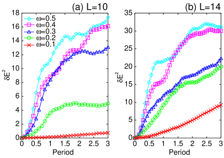
Figure 1: (Color online) Time evolution of energy diffusion for (a) $L=10$ and (b) $L=14$. The parameters are the following: $J_{1}=J_{2}=1.0$, $\Delta=0.3$, $B_{0}=1.0$.

We calculate time evolution of the state and evaluate energy variances at each integer multiple of the effective period $T^{\prime}=T/L=2\pi/(\omega L)$. As mentioned already, we choose the ground state as an initial state, following the spirit of real physics of condensed matters. This viewpoint is in contrast to that of the random matrix models where initial states are chosen among high-lying ones. Wilkinson88 ; WilAus92 ; WilAus95 ; Bulgac ; Cohen00D ; Cohen00M Consequently, the energy variance of our primary concern is the variance around the ground state energy $E_{0}$ and is defined by

$$\delta E(t)^{2}=\langle\psi(t)|[H(t)-E_{0}]^{2}|\psi(t)\rangle.$$ (10)

Time evolution of $\delta E(t)^{2}$ is shown in Fig. 1. The parameters except for $\omega$ are fixed. The larger $\omega$ is, the faster the energy diffusion grows, which is consistent with our expectations. The details will be explained in Sec. IV. For wide parameter values of the next-nearest-neighbor (NNN) coupling $J_{2}$ and exchange anisotropy $\Delta$, the early stage of quantum dynamics becomes to show the normal diffusion in energy space, i.e., a linear growth of $\delta E(t)^{2}$ in time. While we proceed to investigate this normal diffusion process, energy variances will finally saturate because the system size we consider is finite. On the other hand, energy variances can also saturate because of another reason, i.e., the dynamical localization effect associated with a periodic perturbation.

During the first period, $\delta E(t)^{2}$ shows a linear growth in time as shown in Fig. 1 (a). The range of the linear growth is not sufficiently wide because the number of levels is not large enough for $L=10$. However, if the number of levels as well as the system size is increased, the length of a linear region may be elongated. In fact, the linear growth of $\delta E(t)^{2}$ during the first period can be recognized more clearly for $L=14$ than for $L=10$ [see Fig. 1 (b)]. The diffusion coefficient has to be determined much earlier than the time where saturation begins. We determine the diffusion coefficient $D$ from the fitting

$$\delta E(t)^{2}=Dt+\mbox{\rm const.}$$ (11)

to some data points around the largest slope in the first period, where the normal diffusion is expected.

IV Diffusion coefficients: dependence on field strength and frequency

Since the time evolution of our system starts from the ground state, we consider non-adiabatic regions where inter-level transitions frequently occur. In other words, we suppress a near-adiabatic or the so-called Landau-Zener (LZ) region where the driving frequency $\omega$ is much smaller than the mean level spacing divided by Planck constant. Because of a large energy gap between the ground and first excited states, the near-adiabatic region cannot result in the notable energy diffusion and will be left outside a scope of the present study.

Beyond the LZ region, however, so long as the changing rate $\dot{X}$ of a perturbation parameter is not very large, note2 the diffusion coefficient can be calculated using the Kubo formula. We call such a parameter regime “linear response” regime. In the linear response regime, $D\propto\dot{X}^{2}$ (See, e.g., Refs. WilAus92, and WilAus95, ). When $\dot{X}$ is large, however, the perturbation theory fails. We call such a parameter regime “non-perturbative” regime. In the non-perturbative regime, the diffusion coefficient is smaller than that predicted by the Kubo formula. WilAus95 ; Cohen00D According to Ref. WilAus95, , $D\propto\dot{X}^{\gamma}$ with $\gamma\leq 1$ in the non-perturbative regime. We note that $\dot{X}\propto B_{0}\omega$ in this paper since the perturbation is given by Eq. (4). Both Refs. WilAus95, and Cohen00D, are based on the random matrix models, which are utterly different from our deterministic one.

Figure 2: Driving frequency dependence of the diffusion coefficients. The chained line and the solid line are just eye guides for $D\propto\omega^{\beta}$ with $\beta=1$ and $2$, respectively. The symbols ($\diamond$) are the average of the diffusion coefficients calculated for several values of $\Delta$ ($0.3\leq\Delta\leq 0.8$). The parameters are the following: $L=10$, $J_{1}=1.0$; (a) $J_{2}=1.0$, (b) $J_{2}=0.2$.

Figure 3: Dependence of the diffusion coefficients on the product of field strength $B_{0}$ and driving frequency $\omega$ for (a) $L=10$ and (b) $L=14$. The symbols ($\diamond$) are the average of the diffusion coefficient calculated for several values of $\Delta$ ($0.3\leq\Delta\leq 0.8$). The parameters are $J_{1}=J_{2}=1.0$; for the inset, $J_{1}=1.0$ and $J_{2}=0.2$. The chained line and the solid line are just eye guides for $D\propto(B_{0}\omega)^{\beta}$ with $\beta=1$ and $2$, respectively. Some error bars are too short to see.

Numerical results of diffusion coefficients in Fig. 2 are almost consistent with the argument of Ref. WilAus95, . Diffusion coefficients as a function of $\omega$ are shown in Fig. 2. In Fig. 2(a), where $J_{2}=1.0$ (i.e., the fully-frustrated case), $D$ is larger as $B_{0}$ is larger for a fixed value of $\omega$. In a small-$\omega$ regime, $D\propto\omega^{\beta}$ with $\beta=2$, though $\beta>2$ for small $B_{0}$. The latter is merely attributed to the fact that the perturbation is too small to observe a sufficient energy diffusion when both $\omega$ and $B_{0}$ are small. In a large-$\omega$ regime, $\beta=1$. Namely, we observe that $\beta=2$ in the linear response regime and $\beta=1$ in the non-perturbative regime. In fact, for a large-$\omega$ regime, the increase of energy variances per effective period hardly depend on $\omega$ by the time when $\delta E(t)^{2}$ starts to decrease. This explains the observation that $D\propto\omega^{\beta}$ with $\beta=1$ in both Fig. 2(a) and Fig. 2(b). Let us represent the increase of energy variances per effective period as $\Delta(\delta E^{2})$. From the definition of $D$, i.e. Eq. (11), $D\propto\Delta(\delta E^{2})/T^{\prime}$. If $\Delta(\delta E^{2})$ is constant, $D\propto\omega$.

On the other hand, in Fig. 2(b) where $J_{2}=0.2$ (i.e., a weakly-frustrated case), the region with $\beta=1$ is expanding. For small $B_{0}$, $\beta>2$ in a small-$\omega$ regime is the same as in the case of $J_{2}=1.0$. For small $B_{0}$ and around $\omega\sim 1$, $D$ seems to rather decrease than increase especially in the case of $J_{2}=0.2$. Some kind of localization would have occurred in the very early stage of energy diffusion for large $\omega$ and small $B_{0}$, leading to the suppression of $D$.

It is seen more clearly in Fig. 3 how the behavior of $D$ changes between a linear response regime and a non-perturbative regime. The diffusion coefficient $D$ obeys the power law $D\propto(B_{0}\omega)^{\beta}$ with its power $\beta$ being two in the linear response regime and $\beta=1$ in the non-perturbative regime. For small $B_{0}\omega$, the power law seems to fail because of some finite-size effects. These universal feature is confirmed in systems of larger size. Actually, $D$ obeys the power law better for $L=14$ [Fig. 3(b)] than $L=10$ [Fig. 3(a)]. In addition, error bars are shorter for $L=14$ than $L=10$. Here, we have used the data of $\omega\leq 1$. We cannot expect meaningful results in a large-$\omega$ regime since, as mentioned above, energy diffusion is not normal there.

Figure 3 suggests that the strength of frustration should affect the range of the linear response regime. The linear response regime is shorter for $J_{2}=0.2$ than for $J_{2}=1.0$, while the non-perturbative regime is larger for $J_{2}=0.2$ than for $J_{2}=1.0$. In fact, when $J_{2}=0$ (i.e. the integrable case), $D\propto(B_{0}\omega)^{\beta}$ with $\beta=1$ for almost all the data in the same range of $B_{0}\omega$ as that of Fig. 3.

V Oscillation Of energy diffusion in weakly-frustrated cases

We shall now proceed to investigate oscillations of diffusion which occur in the non-perturbative regime of a weakly-frustrated case. Figure 4(a) shows an example of oscillatory diffusion for $J_{2}=0.2$, which is compared with a non-oscillatory diffusion for $J_{2}=1.0$. The two examples have the same set of parameters except for $J_{2}$. However, the cases of $J_{2}=1.0$ and $J_{2}=0.2$ are in the linear response regime and in the non-perturbative regime, respectively. The variance for both cases shows normal diffusion at the very early stage of time evolution. For $J_{2}=1.0$, the energy variance seems to saturate after a normal diffusion time. On the contrary, the energy variance for $J_{2}=0.2$ shows large-amplitude oscillations. To investigate more details, we introduce another definition of energy variance:

$$\delta\tilde{E}(t)^{2}=\langle\psi(t)|[H(t)-\langle\psi(t)|H(t)|\psi(t)\rangle]^{2}|\psi(t)\rangle.$$ (12)

This follows a standard definition of the variance and quantifies the degree of energy diffusion around the time-dependent expectation of the energy Hamiltonian. The time evolutions of $\delta\tilde{E}(t)^{2}$ corresponding to that of $\delta E(t)^{2}$ are shown in Fig. 4(b). In the fully-frustrated case ($J_{2}=1.0$), the profile of $\delta\tilde{E}(t)^{2}$ is similar to that of $\delta E(t)^{2}$. This observation indicates that an occupation probability spread over the whole levels after normal diffusion of energy.

Figure 4: Examples for time evolution of energy variances : (a) $\delta E(t)^{2}$ and (b) $\delta\tilde{E}(t)^{2}$ (see text). Solid lines are for $J_{2}=1.0$; Broken lines, $J_{2}=0.2$. The parameters are the following: $L=10$, $J_{1}=1.0$, $\Delta=0.3$, $B_{0}=1.5$, $\omega=0.5$.

On the contrary, in a weakly-frustrated case ($J_{2}=0.2$) in Fig. 4, $\delta\tilde{E}(t)^{2}$ shows small-amplitude oscillations reflecting the large-amplitude oscillations of $\delta E(t)^{2}$. Most part of $\delta\tilde{E}(t)^{2}$ for $J_{2}=0.2$ is smaller than that for $J_{2}=1.0$. Furthermore, minima of $\delta\tilde{E}(t)^{2}$ come just before minima and maxima of $\delta E(t)^{2}$. These observations indicates the following: an occupation probability, which is diffusing slowly, clustering around the expectation of energy oscillates together with the expectation in the energy space. To make the picture of such behavior clearer, let us consider an occupation probability described by

$$P_{t}(E_{n})=|\langle\phi_{n}|\psi(t)\rangle|^{2},$$ (13)

where $|\phi_{n}\rangle$ is the $n$th excited eigenstate of $H_{0}$:

$$H_{0}|\phi_{n}\rangle=E_{n}|\phi_{n}\rangle.$$ (14)

When $t=0$ , $P_{t}(E_{n})$ is given by the Kronecker delta: $P_{0}(E_{n})=\delta_{E_{n},E_{0}}$, where $E_{0}$ is the energy of the ground state. As $t$ increases, $P_{t}(E_{n})$ forms a wave packet in energy space and moves to higher levels. When the wave packet reaches some highest level, it reflects like a soliton and moves back to lower levels. Such behavior is repeated, although the wave packet of $P_{t}(E_{n})$ broadens slowly. We have actually watched this soliton-like behavior of $P_{t}(E_{n})$ in a form of an animation.

Figure 5: Parts of energy spectra depending on adiabatically fixed time $t$ with $0\leq t\leq T/4$. Effective period is $\omega T^{\prime}=2\pi/10$. The parameters are the following: $L=10$, $J_{1}=1.0$, $\Delta=0.3$, $B_{0}=0.8$; (a) $J_{2}=1.0$, (b) $J_{2}=0.2$.

The picture discussed above is also supported by the adiabatic energy spectra in Fig. 5. Figures 5(a) and 5(b) correspond to fully- and weakly-frustrated cases, respectively. Much more sharp avoided crossings appear in Fig. 5(b) than Fig. 5(a). Some energy levels appear to be crossing, although they are very close and never crossing in fact. At a sharp-avoided-crossing point, Landau-Zener formula for two adjacent levels is applicable. Then the nonadiabatic transition leads to one-way transfer of a population from a level to its partner, failing to result in the energy diffusion. For small-$J_{2}$, therefore, successive sharp avoided crossings can suppress diffusion of energy.

We believe that large-amplitude oscillations of $\delta E(t)^{2}$ should be one of characteristic features of the non-perturbative regime in this finite frustrated spin system. In fact, similar oscillations of energy variance are seen for large $\omega$ and large $B_{0}$ even when $J_{2}=1.0$ though the energy variance rapidly converges after one or two periods. How long such oscillations continue should depend mainly on $J_{2}$.

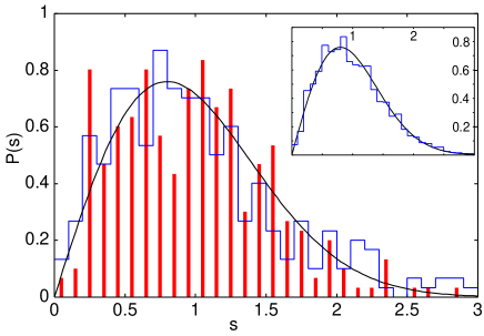
Figure 6: (Color online) Level-spacing distributions at $t=\pi/4$ for lowest 300 levels from the ground state (about 10% of all 3003 levels). Blue histogram is for $J_{2}=1.0$; Red bars, $J_{2}=0.2$; Solid curve, GOE spectral statistics. The other parameters are the following: $L=14$, $S^{z}_{\rm tot}=1$, $J_{1}=1.0$, $\Delta=0.3$, $B_{0}=0.8$. The inset is for all levels when $J_{2}=1.0$. The numerical methods to obtain the level-spacing distributions are referred in Refs. Kudo03, ; Kudo04, .

It is a notable fact that, common to both $J_{2}=1.0$ and $J_{2}=0.2$, the level-spacing distributions in Fig. 6 show GOE behavior. This GOE behavior in the adiabatic energy spectra appears for an arbitrary fixed time except for special points such as $t=T=2\pi/\omega$. This fact suggests that dynamics can reveal some various generic features of quantum many-body systems which can never be explained by level statistics. The level-spacing distributions in Fig. 6 convey another crucial fact: they have been calculated for low energy levels because our interest is in the low energy region around the ground state. We have confirmed that the level-spacing distributions for all energy levels in the inset is also described by GOE spectral statistics. It is typical of this frustrated spin system that GOE level statistics is observed already in the low energy region. Kudo04

VI Conclusions

We have explored the energy diffusion from the ground state in frustrated quantum $XXZ$ spin chains under the applied oscillating magnetic field. In a wide parameter region of next-nearest-neighbor (NNN) coupling $J_{2}$ and exchange anisotropy $\Delta$, the diffusion is normal in the early stage of diffusion. Diffusion coefficients $D$ obey the power law with respect to both the field strength and driving frequency with its power being two in the linear response regime and equal to unity in the non-perturbative regime. In the case of weakened frustrations with small-$J_{2}$ we find oscillation of energy diffusion, which is attributed to a non-diffusive and ballistic nature of the underlying energy diffusion. In this way, the energy diffusion reveals generic features of the frustrated quantum spin chains, which cannot be captured by the analysis of level statistics.

- (1) See articles in Quantum Chaos Y2K, Proceedings of Nobel Symposium edited by K. F. Berggren and S. Åberg (Royal Swedish Academy of Sciences/World Scientific, Singapore, 2001).
- (2) G. Jona-Lasinio and C. Presilla, Phys. Rev. Lett. 77, 4322 (1996).
- (3) T. Prosen, Phys. Rev. Lett. 80, 1808 (1998); T. Prosen, Phys. Rev. E 60, 3949 (1999).
- (4) V. V. Flambaum and F. M. Izrailev, Phys. Rev. E 64, 026124 (2001).
- (5) M. Wilkinson, J. Phys. A 21, 4021 (1988).
- (6) M. Wilkinson and E. J. Austin, Phys. Rev. A 46, 64 (1992).
- (7) M. Wilkinson and E. J. Austin, J. Phys. A 28, 2277 (1995).
- (8) A. Bulgac, G. D. Dang, and D. Kusnezov, Chaos, Solitons and Fractalts 8, 1149 (1997).
- (9) D. Cohen and T. Kottos, Phys. Rev. Lett. 85, 4839 (2000).
- (10) D. Cohen, F. M. Izrailev, and T. Kottos, Phys. Rev. Lett. 84, 2052 (2000); D. Cohen, Lecture Notes in Physics 597 edited by P. Garbaczewski and R. Olkiewicz, p. 317 (2002).
- (11) M. Machida, K. Saito, and S. Miyashita, J. Phys. Soc. Jpn. 71, 2427 (2002).
- (12) H. Kikuchi, H. Nagasawa, Y. Ajiro, T. Asano, and T. Goto, Physica B 284-288, 1631 (2000).
- (13) M. Hagiwara, Y. Narumi, K. Kindo, N. Maeshima, K. Okunishi, T. Sakai, and M. Takahashi, Physica B 294-295, 83 (2001).
- (14) Y. Kitaoka et al., J. Phys. Soc. Jpn 67, 3703 (1998); V. P. Plakhty, J. Kulda, D. Visser, E. V. Moskvin, and J.Wosnitza, Phys. Rev. Lett. 85, 3942 (2000); A. Lascialfari, R. Ullu, M. Affronte, F. Cinti, A. Caneschi, D. Gatteschi, D. Rovai, M. G. Pini, and A. Rettori, Phys. Rev. B 67, 224408 (2003).
- (15) K. Nakamura, Y. Nakahara, and A. R. Bishop, Phys. Rev. Lett. 54, 861 (1985); K. Nakamura, Quantum Chaos (Cambridge University Press, Cambridge, 1993).
- (16) H. Yamasaki, Y. Natsume, A. Terai, and K. Nakamura, J. Phys.: Condens. Matter 16, L395 (2004).
- (17) K. Kudo and T. Deguchi, Phys. Rev. B 68, 052510 (2003).
- (18) K. Kudo and T. Deguchi, arXiv: cond-mat/0409761.
- (19) On the contrary, the corresponding integrable spin chains without NNN coupling obey Poissonian level statistics, except when they commute with the loop algebra. Kudo03 (About the loop algebra, see: T. Deguchi, K. Fabricius, and B. M. McCoy, J. Stat. Phys. 102, 701 (2001)).
- (20) Actually, GOE behavior has not appeared in Ref. Kudo03, . In Ref. Kudo04, , it is resolved why GOE behavior did not appear, and GOE behavior is really shown.
- (21) K. Nomura and K. Okamoto, J. Phys. A 27, 5773 (1994).
- (22) M. Suzuki: Phys. Lett. A 146, 319 (1990).
- (23) More precisely, this phrase means that the time scale upon which the time-dependent Hamiltonian matrix elements decorrelate is much larger than the time scale corresponding to the typical separation of energy levels.