Dynamic response of trapped ultracold bosons on optical lattices

Abstract

We study the dynamic response of ultracold bosons trapped in one-dimensional optical lattices using Quantum Monte Carlo simulations of the boson Hubbard model with a confining potential. The dynamic structure factor reveals the inhomogeneous nature of the low temperature state, which contains coexisting Mott insulator and superfluid regions. We present new evidence for local quantum criticality and shed new light on the experimental excitation spectrum of ⁸⁷Rb atoms confined in one dimension.

The advent of Bose–Einstein condensation in cold atomic gases opened new fields of research merging atomic physics and quantum optics with condensed matter physics. Scattering experiments common in solid state physics and liquid helium have been adapted to extract information on excitation dynamics of atomic condensates resulting in the technique of Bragg spectroscopy Braggspec . Initial experiments on Bose-condensed gases could be well described by mean-field Gross-Pitaevskii approaches, valid for weak interactions. However, recent experiments have reached the regime of strongly interacting atoms, often by confining the atoms in optical lattices, leading, for instance, to the destruction of a phase-coherent superfluid (SF) phase and the establishment of Mott insulator (MI) phase with squeezed number fluctuations NatGreiner ; StofEss04 ; NatParedes . The latter state is considered as promising for use as a large quantum register for quantum information purposes JakschQI .

Ultracold atoms in optical lattices are an almost ideal realisation of the boson Hubbard model Jaksch98 , that has previously been studied intensely (with different motivation) FisherM ; GGBRTS90 . Much of this previous work focussed on the equilibrium phase diagram or on the conductivity in the presence of disorder. However, as in other condensed matter systems, a rich source of information on the excitation dynamics is the dynamic structure factor, the double Fourier transform of density-density correlations, which can be measured using Bragg spectroscopy Braggspec ; DSFBH ; roth . It is therefore of great current interest to study the dynamic structure factor of the boson Hubbard model. Because of loss of translational invariance due to the presence of the confining trap, results for the uniform system cannot be directly applied to the confined system. This affects both the static response, the system no longer has a globally incompressible phasePRL02 , and the dynamics, since the wave vector is no longer a good quantum number.

In this paper, we use Quantum Monte Carlo to study the ground state of the one-dimensional boson-Hubbard model in a confining harmonic potential:

$$H = -t\sum_{i}\left(a^{\dagger}_{i}a_{i+1}+a^{\dagger}_{i+1}a_{i}\right)+$$ (1)

$$V_{T}\sum_{i}(x_{i}-\frac{L}{2})^{2}\,n_{i}+U\sum_{i}n_{i}(n_{i}-1).$$

where $L$ is the number of sites and $x_{i}$ is the coordinate of the $i$th site. The hopping parameter, $t$, sets the energy scale, $n_{i}=a^{\dagger}_{i}a_{i}$ is the number operator, $[a_{i},a^{\dagger}_{j}]=\delta_{ij}$ are bosonic creation and destruction operators. $V_{T}$ sets the confining trap curvature, while the contact interaction is given by $U$. We use the World Line algorithm for our simulations. The static properties and state diagram of this model were studied in PRL02 where it was shown, among other things, that the presence of the trap and the destruction of translation invariance eliminate the quantum phase transitions between the SF and MI phases and replace it by a co-existence of phases. Our main results are: (i) due to co-existence of MI and SF regions in the confined system, the dynamic structure factor exhibits two excitation branches, one gapped and one with a linear, phonon-like, dispersion; (ii) these branches are shown clearly to be connected to the spatial regions containing the MI and SF phases and (iii) by using an appropriate measure of local excitations, we provide new evidence for local quantum criticality.

In the ground state ($T=0$) the dynamic structure factor is given by

$$S(k,\omega) = \frac{1}{L^{2}L_{t}}\sum_{t}\sum_{r,r^{\prime}}{\rm e}^{-i\omega t}{\rm e}^{ik(r-r^{\prime})}$$ (2)

$$\times\langle n(r,0)n(r^{\prime},t)\rangle$$

$$= \sum_{m}\delta(\omega-E_{m}+E_{0})|\langle 0|n(k,0)|m\rangle|^{2},$$ (3)

where $L_{t}$ is the number of time slices, $E_{m}$ the energy of state $|m\rangle$, and $\langle n(r,0)n(r^{\prime},t)\rangle$ the space and time separated density-density correlation function. With our normalization we have $\int{\rm d}\omega S(k,\omega)=N_{b}S(k)$ where $S(k)$ is the static structure factor and $N_{b}$ the number of bosons. Equation (3) shows that, for a given $k$, the peaks in $S(k,\omega)$ correspond to the excitation energies. We have performed all our simulations at $\beta=T^{-1}=10$ and verified that it is sufficient to study the ground state. In the World Line algorithm, it is a simple matter to measure $\langle n(r,0)n(r^{\prime},\tau)\rangle$ where $\tau$ is the imaginary time separation. The dynamic structure factor is then given by Eq. (2), with $t$ replaced by $-i\tau$ which then requires the performance of a Laplace, instead of a Fourier, transform. This is done with the help of the stochastic method (SM) stochastic .

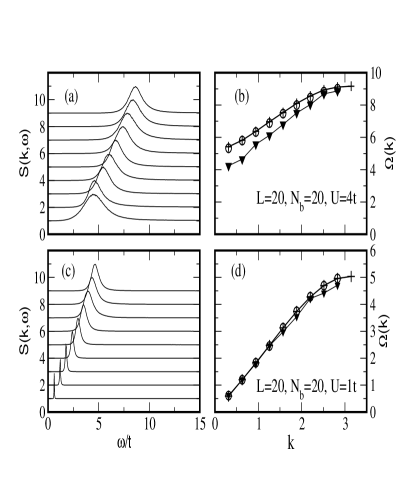
Figure 1: (a,c) $S(k,\omega)$ vs $\omega$ and (b,d) $\Omega(k)$ vs $k$ for $k=2\pi n/L$ with $1\leq n\leq 9$. The system has commensurate filling: $L=20,N_{b}=20,\beta=10$ with $U=4t$ (a,b) and $U=1t$ (c,d).

Figure 1 shows $S(k,\omega)$ for the uniform system in the MI (a) and SF (c) phases. The critical value in one dimension is $U_{crit}=2.33t$ monien . For better visibility, our $S(k,\omega)$ curves in Figs. 1,3 have been normalized $\sum_{\omega}S(k,\omega)=1$ and do not show the true spectral weights. For the SF, it is clear that the excitation energies for small $k$ are linear in $k$, i.e. phononic, leading to a stable SF phase (according to the Landau criterion). On the other hand, the MI case clearly shows a gap at $\omega\approx 3t$, where the spectral weight in Fig. 1(a) starts to be appreciable. This is in excellent agreement with the value of the gap of $3t$ measured in GGBRTS90 from the static compressibility. Note that the first peak is at $\omega\approx 4.5t$, which is larger than the gap, and that the peaks for the MI are rather wide. This is due to the presence of several closely spaced peaks which we cannot resolve. Such closely spaced peaks are seen in the exact diagonalization of smaller systems roth where, for the MI, the first in the lowest group of peaks does indeed correspond to the gap.

One can study the excitation spectrum using the dispersion relation $\Omega(k)$,

$$\Omega(k)=\frac{\int{\rm d}\omega\,\,\omega\,S(k,\omega)}{\int{\rm d}\omega\,\,S(k,\omega)},$$ (4)

which can be expressed in terms of purely static quantities using the $f$-sum rule

$$\int_{-\infty}^{+\infty}{\rm d}\omega\,\,\omega\,S(k,\omega)=N_{b}E_{k},$$ (5)

$$E_{k}=\frac{-t}{L}\left({\rm cos}(2\pi k/L)-1\right)\langle 0|\sum_{i=1}^{L}\left(a^{\dagger}_{i}a_{i+1}+a^{\dagger}_{i+1}a_{i}\right)|0\rangle.$$ (6)

The dispersion relation is then given by the Feynman result,

$$\Omega(k)=\frac{E_{k}}{S(k)}.$$ (7)

Figure 1 shows $\Omega(k)$ obtained using the dynamic structure factor, Eq. (4) (circles), and also using only static quantities, Eqs. (6) and  (7) (pluses) in the MI (b) and SF (d) phases. These two calculations agree very well and give for the SF phase linear dispersion for small $k$ and a gap for the MI. While $\Omega(k)$ shows clearly the presence of a gap for MI, it does not give its value since it is an integral over all peaks that may be present. In addition, we show the positions of the peaks in both cases (down triangles) which agree extremely well with $\Omega(k)$ when the peaks are very sharp. This offers a consistency and precision check on our methods. Our results for $\Omega(k)$ agree with the small lattice exact diagonalization results roth .

We now turn to the confined system where we always take a system size $L=100$ and $V_{T}=0.008$. These values and the fillings we use are comparable to the experimental ones. Figure 2 shows the local density profiles for a system in a pure SF phase, (a), and with coexistence of SF and MI, (b). Figure 3 shows the corresponding $S(k,\omega)$. For the pure SF case, Fig. 3(a), $S(k,\omega)$ is similar to the SF case in Fig. 1(c): no gap is visible and the excitation energies go to zero smoothly as $k\to 0$. Figure 3(b) shows the same for $N_{b}=64$ where there is coexistence of MI and SF phases. There is a marked difference in the behavior of $S(k,\omega)$ compared to the pure SF case: two branches of excitation peaks are clearly visible in the form of two ridges. The low energy branch is seen to be very similar to $S(k,\omega)$ in the SF case, Fig. 3(a), saturating at about $\omega\approx 3t$, and going smoothly to zero. The second family of peaks saturates at a higher energy, $\omega\approx 8t$ and seems to make its first appearance at about $k\approx 11$ in units of $2\pi/L$ with an $\omega\approx 3t$.

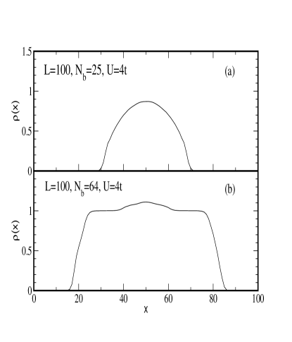
Figure 2: Local density profile, $\rho(x)$, for the confined system with $L=100$, $V_{T}=0.008$, $U=4t$: (a) $N_{b}=25$ (pure SF) and (b) $N_{b}=64$ (co-existence SF-MI).

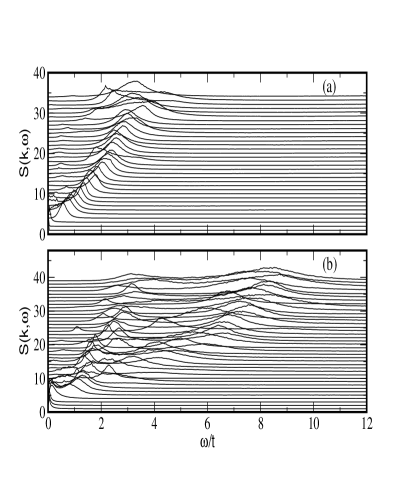
Figure 3: $S(k,\omega)$ vs $\omega$ ($k=2\pi n/L$) for the system in Fig. 2, $N_{b}=25$ (a) and $N_{b}=64$ (b). The two ridges in (b) reflect the SF-MI co-existence, Fig. 2(b).

To interpret these two excitation branches, we examine $S(x,\omega)$, the imaginary time Laplace transform of $\langle n(x,0)n(x,\tau)\rangle$, the same site but time-separated density-density correlation function. This is shown in Fig. 4 which clearly identifies excitation branches with position in the trap. $S(x,\omega)$ includes contributions from all $k$ values. The very low energy phonon excitations arise from the SF regions in the outer wings and the center of the system. The middle excitations, $\omega\sim 2t-3t$ appear prominently in the squeezed SF region between the MI and the outer edges of the system. The value of $\omega$ at the peak corresponds well to the saturation value, at high $k$, of the SF branch of $S(k,\omega)$ in Fig. 3. This effect was observed in all our simulations where a MI phase is present. In these outer regions the superfluid is squeezed between the MI and the rapidly increasing confining potential which appears to enhance the spectral weight of the high $\omega$ excitations and make them so prominent. Finally, the peaks in the two MI regions in Fig. 4 agree well with the saturation value of the higher $\omega$ branch in Fig. 3(b). This confirms our interpretation that this branch corresponds to excitations in the Mott phase. As further evidence, we mention that the $S(x,\omega)$ for the uniform system in the MI phase at $U=4t$ (Fig. 1(a)) has its peak at $\omega\approx 8t$, like the Mott regions in Fig. 3(b).

The interpretation of the higher $\omega$ excitation branch in $S(k,\omega)$ as being due to the MI regions (Fig. 4) and the absence of a gap in Fig. 3 show that even when MI regions are present, the system is gapless! Figure 4 shows that local excitation energies in the MI regions correspond to those in MI phase of the uniform system at the same $U$.

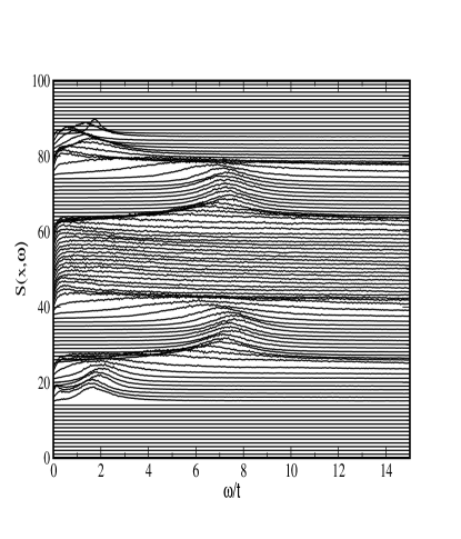
Figure 4: $S(x,\omega)$ for the system in Fig. 3(b) and shows the origin of gapped and ungapped excitation branches are the SF and MI regions.

Another very striking feature in Fig. 4 is the behavior of $S(x,\omega)$ at the boundary between SF and MI sites: The peak in $S(x,\omega)$ is very broad and extends from $\omega=0$ to the largest values examined ($\omega=20t$) which indicates a diverging correlation length in the time direction, $\xi_{t}(x)$. A diverging $\xi_{t}$ means that $\langle n(x,\tau)n(x,0)\rangle$ decays as a power law in $\tau$ and characterizes a quantum phase transition. In this case, since it happens only locally, the divergence of $\xi_{t}(x)$ is renewed evidence of the local quantum criticality already discussed in PRL02 ; rigol .

To measure the total response of the system, summed over all momenta, we use

$$S(\omega)\equiv\sum_{k}S(k,\omega).$$ (8)

This quantity is shown in Fig. 5 for the system shown in Fig. 3(b) (same as Fig. 4) and also for $N_{b}=50,\,U=7t$ which has pure MI in the center surrounded by SF at the edges. A two peak structure is seen where the first peak appears not to depend on $U$ whereas the second peak does. The first peak, therefore, is due to the SF component of the system and has an $\omega$ which corresponds very well to the saturation value of the SF branches of $S(k,\omega)$ in Figs. 3(a,b). On the other hand, the higher peaks depend on the value of $U$ and both correspond to the saturation values of the MI branches in $S(k,\omega)$ (see Fig. 3(b)). Both peaks come from the high $k$ values of the SF and MI branches because those values have the larger spectral weights which therefore dominate when the sum over $k$ is taken. Recall that the $S(k,\omega)$ in the figures have been rescaled for better visibility and do not show the true spectral weights, but Fig. 5 does.

Our two-peak structure, Fig. 5, resembles the excitation spectrum in Fig.2(a) in StofEss04 for ⁸⁷Rb on one-dimensional lattices. Both quantities measure the total response of the system to a given frequency, but they are not the same and the connection between them is not clear. Although $S(k,\omega)$ does detect the presence of MI regions, it also shows there is no overall gap but that local excitation energies do correspond to gap energies in the uniform system at the same $U$. It is possible that the SF peak we detect is missed by reference StofEss04 because the amplitude with which they shake their system is very large ($20\%$ of the optical lattice potential).

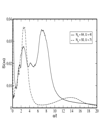
Figure 5: $S(\omega)$ for $N_{b}=64,\,U=4t$ and for $N_{b}=50,\,U=7t$ which has only a MI in the middle.

We have presented the first Quantum Monte Carlo study of the dynamical structure factor, $S(k,\omega)$, for the Hubbard model on uniform and confined optical lattices. The uniform system exhibits linear dispersion (phonons) for the SF and a clear excitation gap in the MI in agreement with the directly computed gap GGBRTS90 . In the absence of MI regions in the confined system, the $S(k,\omega)$ behavior is very similar to the uniform case.

However, when MI regions are present (Figs. 3(b) and 4), we find that although $S(k,\omega)$ shows the presence of such regions, it also clearly shows the absence of a gap: the system is globally compressible and gapless PRL02 . The presence of the MI regions is deduced from the presence of two excitation branches in $S(k,\omega)$ or from the double peak structure of $S(\omega)$ (Fig. 5). We note, as discussed above, that the second peak in Fig. 5 corresponds to MI regions. In addition, we note that $S(k,\omega)$ and $S(\omega)$ give information about local excitations in the trap. For example, by comparing $S(k,\omega)$ with $S(x,\omega)$ (Figs. 3(b) and 4) we have found that the first peak in $S(\omega)$ represents excitations in the SF regions at the edges of the system while the second peak represents the excitations in the MI regions. The value of the local excitation energy is consistent with the gap value for the uniform system at the same $U$. This is consistent with the local quantum criticality view PRL02 ; rigol for which we present new compelling evidence in Fig. 4. Our conclusions can be tested experimentally since the dynamic structure factor $S(k,\omega)$ (and therefore, $S(\omega)$) can be measured experimentally using Bragg spectroscopyBraggspec ; DSFBH .

Acknowledgements We acknowledge helpful discussions with M. Troyer, H.T.C. Stoof and C. Checker. R.T.S. was supported by NSF-DMR-0312261 and NSF-INT-0124863, PJHD is supported by Stichting FOM.

References

- (1) J. Stenger et al., Phys. Rev. Lett. 82, 4569 (1999); D.M. Stamper-Kurn et al., ibid 83, 2876 (1999).
- (2) M. Greiner et al., Nature 415, 39 (2002).
- (3) T. Stöferle et al., Phys. Rev. Lett. 92, 130403 (2004).
- (4) B. Paredes et al., Nature 429, 277 (2004).
- (5) D. Jaksch et al., Phys. Rev. Lett. 82, 1975 (1999).
- (6) D. Jaksch et al., Phys. Rev. Lett. 81, 3108 (1998).
- (7) M.P.A. Fisher et al., Phys. Rev. B40, 546 (1989).
- (8) G.G. Batrouni et al., Phys. Rev. Lett. 65, 176 (1990).
- (9) J Steinhauer et al., ibid 88, 120407 (2002); D. van Oosten et al., Phys.Rev. A71, 021601(R) (2005).
- (10) R. Roth and K. Burnett, J.Phys.B: At. Mol. Opt.Phys. 37, 3893 (2004).
- (11) G.G. Batrouni et al., Phys. Rev. Lett. 89, 117203 (2002).
- (12) K. S. D. Beach, cond-mat/0403055.
- (13) J. K. Freericks and H. Monien, Phys. Rev. B53, 2691 (1996).
- (14) M. Rigol et al., Phys. Rev. Lett. 91, 130403 (2003).