Correlated mesoscopic fluctuations in integer quantum Hall transitions

Abstract

We investigate the origin of the resistance fluctuations of mesoscopic samples, near transitions between Quantum Hall plateaus. These fluctuations have been recently observed experimentally by E. Peled et al. [Phys. Rev. Lett. 90, 246802 (2003); ibid 90, 236802 (2003); Phys. Rev. B 69, 241305(R) (2004)]. We perform realistic first-principles simulations using a six-terminal geometry and sample sizes similar to those of real devices, to model the actual experiment. We present the theory and implementation of these simulations, which are based on the linear response theory for non-interacting electrons. The Hall and longitudinal resistances extracted from the Landauer formula exhibit all the observed experimental features. We give a unified explanation for the three regimes with distinct types of fluctuations observed experimentally, based on a simple generalization of the Landauer-Büttiker model. The transport is shown to be determined by the interplay between tunneling and chiral currents. We identify the central part of the transition, at intermediate filling factors, as the critical region where the localization length is larger than the sample size.

I Introduction

The integer quantum Hall effect(von Klitzing et al., 1980) (IQHE) is one of very few instances where quantum effects are dramatically manifested in the macroscopic world: if a two-dimensional electron system (2DES) is placed in a large perpendicular magnetic field $B$, its Hall resistance is quantized with high accuracy to $h/(ne^{2})$, where $n>0$ is an integer. This quantization has been explained, within the non-interacting electron approximation, as a bulk effect, (Středa, 1982) as a topological invariant,(Thouless et al., 1982) and as an edge effect. (Rammal et al., 1983; Büttiker, 1988) The plateau-to-plateau transitions of the Hall resistance, which are accompanied by peaks in the longitudinal resistance, are understood as localization-delocalization transitions with a universal scaling relation.(Pruisken, 1987; Wei et al., 1988; Huckestein and Kramer, 1990; Huo and Bhatt, 1992; Huckestein, 1995)

A different route to observing quantum effects in condensed matter physics, is to reduce the size of the device to the so-called mesoscopic regime. If the size of the device is smaller than the phase coherence length, quantum interference between different paths leads to effects such as random universal conductance fluctuations.Beenakker (1997); Altshuler91 ; Lee87

What happens if the two are combined? The answer was provided by recent IQHE experiments performed on a mesoscopic sample.(Peled et al., 2003a, b; Peled04, ) The expected quantum mechanical interference of electronic wave-functions indeed causes reproducible patterns of fluctuations in the resistances near plateau-to-plateau transitions, as the magnetic field is varied (in macroscopic samples all resistances vary smoothly with $B$). Interestingly, the fluctuations of resistances measured with different combinations of electrical contacts are not independent; instead, various non-trivial correlations were observed.

In this paper, we investigate the mesoscopic IQHE within the non-interacting electron approximation. Our numerical simulations provide the basis for a unified explanation of these novel experimental observations, based on existing theories of the IQHE and mesoscopic transport (some of these results have been summarized in Ref. Zhou04c, ). We begin the paper with a brief review of the experimental observations, in Sec. II. In Sec. III we describe in detail the model we use, and our approach to solve the scattering problem that allows us to compute the conductance matrix from the multi-terminal Landauer formula. Our numerical results, which exhibit all the experimentally observed symmetries and correlations, are presented in Sec. IV. In Sec. V we explain how these various correlations and symmetries arise. We analyze the allowed structure of the conductance matrix, and show how it directly determines the possible correlations between fluctuations of various resistances. Finally, Sec. VI contains the summary and a discussion of the relevance of these results.

II Summary of Experimental results

The experimental sample is an InGaAs/InAlAs heterostructure with impurities (Indium atoms) distributed throughout. As a result, the mobility is rather low (fractional quantum Hall effect is not observed). Even for the IQHE, only the first few plateau-to-plateau transitions can be identified. The experimental setup is sketched in Fig. 1. The Hall bar is connected to six terminals, indexed 1 to 6. The sample is considered mesoscopic because the characteristic size of its central region between the 4 central terminals, of about $2\mu$m, is comparable to the phase coherent length $L_{\phi}\approx 2-3\mu$m.(Peled et al., 2003a, b; Peled04, )

As customary, we denote the various resistances as $R_{ij,mn}=V_{mn}/I_{ij}$, where $V_{mn}=V_{n}-V_{m}$ is the voltage difference measured between terminals $n$ and $m$, when the current is injected in the sample through terminal $i$ and extracted through terminal $j$. For example, to measure the Hall and longitudinal resistances, a small current $I$ is fed into terminal 1 and collected from terminal 4; no net currents are flowing in the other 4 terminals. One can then measure two longitudinal resistances $R^{L}_{14,23}$, $R^{L}_{14,65}$, and two Hall resistances $R^{H}_{14,62}$, $R^{H}_{14,53}$. For any macroscopic sample, the two resistances of each pair are equal. For a mesoscopic sample, however, each resistance exhibits a different fluctuation pattern.(Peled et al., 2003a, b; Peled04, )

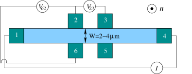
Figure 1: (color online) Typical six-terminal Hall bar used in experiments. In this configuration, the Hall resistance $R^{H}_{14,62}$ and the longitudinal resistance $R^{L}_{14,23}$ are measured.

Another quantity of interest is the “two-terminal resistance” $R_{2t}=R_{63,63}$. Experimentally, it is measured by sending the current from terminal 6 to terminal 3, and measuring the voltage difference between terminal 6 and terminal 3. Because of the two-point measurement, a contact resistance is subtracted from the raw data.Peled et al. (2003b)

Summary of experimental findings:

A: the IQHE transition from the $n^{th}$ to the $n+1^{st}$ plateau, $\forall n>0$, has three distinct regimes:(Peled et al., 2003b; Peled04, )

A1: on the high-$B$ (low filling factor $\nu$) side of the transition, the Hall and the longitudinal resistances have distinct fluctuation patterns, which however are correlated such that:

$$R^{H}_{14,62}+R^{L}_{14,23}=R^{H}_{14,53}+R^{L}_{14,65}={h\over ne^{2}}$$ (1)

A2: in the central part of the transition, the Hall and the longitudinal resistances still exhibit distinct fluctuation patterns, but Eq. (1) is no longer satisfied.

A3: on the low-$B$ (high filling factor $\nu$) side of the transition, the Hall resistances become quantized to the expected plateau value $R^{H}_{14,62}=R^{H}_{14,53}=h/[(n+1)e^{2}]$. The two longitudinal resistances exhibit significant, but this time identical fluctuation patterns, with a maximum amplitude $h/[n(n+1)e^{2}]$, i.e. the difference between quantized Hall resistances of the two neighboring plateaus.

B: the transition inside the lowest Landau level $n=0$ shows the equivalent of A3: at high-$\nu$ one finds the regime where $R^{H}_{14,62}=R^{H}_{14,53}=h/e^{2}$, while the two longitudinal resistances have identical fluctuation patterns with extremely large amplitudes.(Peled et al., 2003a) Regimes A1 and A2 are replaced here by the transition to the insulating phase, where all four resistances increase rapidly with decreasing filling factor.

C: throughout each IQHE transition, the following identity is found to hold to high accuracy:(Peled et al., 2003b)

$$R^{H}_{14,62}+R^{L}_{14,23}=R^{H}_{14,53}+R^{L}_{14,65}=R_{63,63}.$$ (2)

D: Under the reversal of the magnetic field $B\rightarrow-B$, the longitudinal resistances verify the symmetry:(Peled04, )

$$R^{L}_{14,23}(B)=R^{L}_{14,65}(-B),$$ (3)

to high accuracy, although $R^{L}_{14,23}(B)\neq R^{L}_{14,23}(-B)$ and $R^{L}_{14,65}(B)\neq R^{L}_{14,65}(-B)$ except in regime A3, on the high-$\nu$ side of the transition, where the two longitudinal resistances have identical fluctuation patterns.

In the following, we show that all these observations can be explained within the non-interacting electron approximation, using a combination of ideas about the IQHE and mesoscopic transport.

III Numerical simulations

III.1 The conductance matrix and the resistances

The linear response function of the six-terminal Hall bar is the $6\times 6$ conductance matrix $\hat{g}$ that defines the relationship between the currents flowing through the various leads, and their voltages: $I_{\alpha}=\sum_{\beta}g_{\alpha\beta}V_{\beta}$. Here, $I_{\alpha}$ is the current in the lead $\alpha=1,\dots,6$. We use the convention $I>0$ $(I<0)$ for currents coming out of (flowing into) the sample. $V_{\alpha}$ is the voltage of the lead $\alpha$.

Knowledge of the conductance matrix allows us to calculate the various resistances in a straightforward way. In the conventional setup, the current flows from lead 1 to lead 4 and therefore $\hat{I}_{14}=\begin{pmatrix}-I&0&0&I&0&0\end{pmatrix}^{T}$. Without loss of generality, we set $I=1$ (this is a linear response theory) and $V_{4}=0$ (the voltage differences are not affected if one of the terminals is grounded). After solving the $6\times 6$ equation $\hat{g}\hat{V}=\hat{I}_{14}$ for the other 5 voltages, we can directly compute the various resistances from their definitions:

$$R^{L}_{14,23}=V_{2}-V_{3},\;R^{L}_{14,65}=V_{6}-V_{5},$$ (4a)

$$R^{H}_{14,62}=V_{6}-V_{2},\;R^{H}_{14,53}=V_{5}-V_{3}.$$ (4b)

The two-terminal resistance is determined similarly. In this case, the electric currents flow from lead 6 to lead 3: $\hat{I}_{63}=\begin{pmatrix}0&0&I&0&0&-I\end{pmatrix}^{T}$. After solving the equation $\hat{g}\hat{V}=\hat{I}_{63}$ for the corresponding voltage distribution, we can calculate immediately the two-terminal resistance (assuming again that $I=1$):

$$R_{2t}=R_{63,63}=V_{6}-V_{3}.$$ (5)

Clearly, any other measurement can be simulated in a similar fashion within this formalism. All resistances are functions of various elements of the conductance matrix.

At $T=0$, the off-diagonal elements of the conductance matrix $\hat{g}$ are calculatedBaranger and Stone (1989) by solving a multi-channel scattering problem, according to the Landauer-Buttiker formula:

$$g_{\alpha,\beta\neq\alpha}(E_{F})=\frac{e^{2}}{h}\sum_{i,j}\left|t_{\alpha i,\beta j}(E_{F})\right|^{2}.$$ (6)

Here, $t_{\alpha i,\beta j}(E_{F})$ is the amplitude of probability (transmission amplitude) that an electron with the Fermi energy $E_{F}$, which is injected into the sample through the $j^{th}$ transverse channel of lead $\beta$, will scatter out of the sample into the $i^{th}$ transverse channel of lead $\alpha$. The sum over all the transverse channels of the two leads simply gives the total probability $p_{\beta\rightarrow\alpha}(E_{F})$ for the electron with $E_{F}$ to scatter from lead $\beta$ into lead $\alpha$, and thus:

$$g_{\alpha,\beta\neq\alpha}(E_{F})=\frac{e^{2}}{h}p_{\beta\rightarrow\alpha}(E_{F}).$$ (7)

The diagonal elements of the conductance matrix can then be calculated using the restrictions imposed by charge conservation and gauge invariance:Baranger and Stone (1989) $\sum_{\alpha}g_{\alpha\beta}=\sum_{\beta}g_{\alpha\beta}=0$. The diagonal elements are thus

$$g_{\alpha\alpha}=-\sum_{\beta\neq\alpha}g_{\alpha\beta}=-\sum_{\beta\neq\alpha}g_{\beta\alpha}$$ (8)

The finite-temperature generalization in the linear regime is straightforward:

$$g_{\alpha,\beta}(\mu,T)=\int_{-\infty}^{\infty}dEg_{\alpha,\beta}(E)\left[-\frac{df(E)}{dE}\right],$$ (9)

where $f(E)=[\exp(\beta(E-\mu))+1]^{-1}$ is the Fermi distribution, where $\beta=1/(k_{B}T)$ and $\mu$ is the chemical potential.

The strategy for the numerical simulations of the IQHE in mesoscopic samples is thus apparent. We have to solve a complicated, multi-channel scattering problem to find all the amplitudes of transmission through the Hall bar. This allows us to calculate the conductance matrix and therefore the various resistances. This is repeated for many values of the Fermi energy (corresponding to different filling factors $\nu$ of the Landau level) to obtain the the traces of the resistances as $\nu$ changes. We now describe the details of our simulations.

III.2 The model

In this section we describe the model we use to numerically simulate IQHE transitions in mesoscopic samples. This comprises the sample, the confining potential, the disorder potential, the external leads and their contacts to the sample. As already stated, we assume non-interacting electrons – the usual approximation when treating the IQHE. For numerical convenience, we ignore Landau level (LL) mixing, although the whole formalism can be straightforwardly extended to include it. LL mixing can be ignored for large magnetic fields (the case of interest to us), when the cyclotron energy is the largest energy scale in the problem. In the following, we take the effective mass of the electron in the 2DES to be that of GaAs/AlAs heterostructures, $m^{*}=0.067m_{e}$, and use $-e,e>0$ for the electron charge.

III.2.1 The sample

In choosing the sample geometry, we face an apparent problem. On one hand, when working with Landau levels, it is convenient to consider a rectangular sample with periodic boundary conditions along one axis, since in this case the eigenstates of each LL are known analytical functions. This simplifies considerably the calculation of various matrix elements. On the other hand, however, a Hall bar with different contacts on all sides, such as sketched in Fig. 1, is obviously not consistent with periodic boundary conditions.

Our solution is to start with an area larger than the Hall bar itself. For this enlarged area we impose cyclic boundary conditions to generate a convenient basis for the Hilbert subspace of each LL. We then add a confining potential to “carve out” the Hall bar from this larger area. This potential is described in the next subsection.

Consider, then, 2D electrons in an area of size $L_{x}\times L_{y}$, with periodic boundary conditions in the $y$-direction, and placed in a perpendicular magnetic field $B$. The spectrum consists of Landau levels of energy $E_{n\sigma}=\hbar\omega_{c}(n+1/2)-g\mu_{B}B\sigma$, where $n=0,1,2,...$ is the LL index, and $\sigma=\pm 1/2$ is the $z$-axis spin projection. The cyclotron energy is $\hbar\omega_{c}=eB/m^{*}$.

If we use the Landau gauge $\vec{A}=(0,Bx,0)$, the eigenfunctions for the $(n,\sigma)$ Landau level are:Zhou04b

$$\langle{\bf r}|n,X,\sigma\rangle={e^{-i{Xy\over l^{2}}}\over\sqrt{L_{y}}}e^{-{1\over 2l^{2}}\left(x-X\right)^{2}}{H_{n}\left({x-X\over l}\right)\over\sqrt{2^{n}n!\sqrt{\pi}l}}\chi_{\sigma}$$ (10)

where $l=\sqrt{\hbar c\over eB}$ is the magnetic length, $H_{n}(x)$ are Hermite polynomials and $\chi_{\sigma}$ are the $z$-spin eigenstates. The cyclic boundary condition in the $y$-direction require that $X_{j}=j{2\pi l^{2}/L_{y}}$, $j\in Z$. $X_{j}$, the guiding center, characterizes the location at which individual basis states are centered on the $x$-axis [see Eq. (10)]. Since $-L_{x}/2<X_{j}<L_{x}/2$, it follows that $-N/2<j<N/2$, and the degeneracy of each spin-polarized LL is $N=L_{x}L_{y}/(2\pi l^{2})$. As we show later, $N$ roughly defines the size of the matrix involved in solving the scattering problem (several more states on the contacts have to be included as well).

In the simulations shown here, we use $L_{x}=L_{y}=4\mu$m. For a field of several Tesla, this leads to a degeneracy $N\sim 10^{4}$, which can be easily handled by a generic PC cluster in a reasonable amount of time. The main problem is that our sample is shorter than the experimental sample ($4\mu$m instead of $\sim$20$\mu$m). This means that terminals 1 and 4 (see Fig. 1) are much closer to the other 4 terminals than in reality. We fix this problem with the aid of the confining potential, as described in the next subsection.

III.2.2 The confining potential

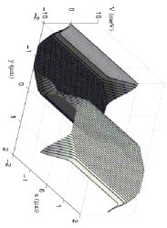
Figure 2: The confining potential $V_{c}(\vec{r})$ that we use. It varies smoothly near the $y$-edges, and has triangular barriers in the corners. See text for details.

As stated before, we add a confining potential $V_{c}(\vec{r})$ to define the Hall bar from the larger area $L_{x}\times L_{y}$ spanned by the LL Hilbert subspace. We have tested several functional forms, to see which are physically reasonable. Some of the choices considered and their pros and cons are discussed in Appendix A.

The confining potential used in simulations is shown in Fig. 2. It is an odd function $V_{c}(x,y)=-V_{c}(x,-y)$ and such that $V_{c}(x,-L_{y}/2)=0$. The Hall bar is the region $-L_{y}/2<y<0/2$ and $-L_{x}/2<x<L_{x}/2$, where the confining potential is:

$$V_{c}(x,y)=-V_{\rm gap}{(1-e^{y/\lambda})(1-e^{-{L_{y}/2+y\over\lambda}})\over 1-e^{-L_{y}/2\lambda}}\times$$

$$\prod_{\nu=\pm 1\atop\mu=0,1}g(|x-\nu L_{x}/2|,|y+\mu L_{y}/2|),$$ (11)

The first line describes the main features: the confining potential is approximatively equal to $-V_{\rm gap}$ inside the Hall bar. We use $V_{\rm gap}=10$ meV in our simulations, which is much larger than the amplitude of the disorder potential (see below). As a result, for Fermi energies $E_{F}<0$, the electrons are confined to the region $[-L_{x}/2,L_{x}/2]\times[-L_{y}/2,0]$ which defines the Hall bar to which contacts will be attached. Near the Hall bar $y$-edges at $y=0,-L_{y}/2$, the confining potential rises smoothly to zero, on a length-scale $\lambda$ (chosen to be 40 nm in our simulations; see discussion in Appendix A). The second line describes the triangular potential barriers added in the four corners of the Hall bar:

$$g(x,y) = \sin^{2}[(x/l_{x}+y/l_{y})\pi/2]\Theta(1-x/l_{x}-y/l_{y})+$$ (12)

$$\Theta(x/l_{x}+y/l_{y}-1),$$

where $l_{x}$ and $l_{y}=L_{y}/6$ define their spatial extension. These barriers help isolate the contacts 1 and 4 from the other contacts, and thus compensate for the shortness of our sample. The alternative is to use a longer sample; this, however, requires significantly more CPU time.

The symmetric choice we made for the confining potential is not necessary; however, it is advantageous for several reasons. If we take the disorder potential such that $V_{d}(x,-y)=-V_{d}(x,y)$ as well, then the particle-hole symmetry of the total potential for the whole sample means that all quantities must be symmetric with respect to $E_{F}=0$. This allows us to check and calibrate the numerical procedure, as discussed in Appendix A.

Another advantage of a symmetric choice is that it allows us to easily define the Hall bar filling factor for $E_{F}<0$, as being twice the filling factor of the LL (same number of filled states, but half the area). Strictly speaking, this is an underestimate. At the Fermi energies $E_{F}\sim-V_{\rm gap}$ of interest to us (see below), the effective area of the Hall bar is somewhat smaller, because of the shape of the confining potential.

III.2.3 The disorder potential

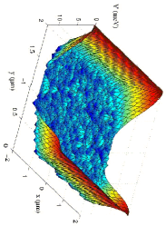
Figure 3: (color online) Total confining plus disorder potential inside the Hall bar, $-L_{y}/2<y<0$ (compare with Fig. 2).

The experimental sample contains many In impurities which serve as short range scattering centers. We simulate a short-range disorder potential $V_{d}(\vec{r})$ by adding 18000 Gaussian scatterers randomly placed inside the Hall bar area $[-2,2]{\rm\mu m}\times[-2,0]{\rm\mu m}$. Each Gaussian scattering potential is of the form $Ae^{-r^{2}/d^{2}}$, where $d$ is uniformly distributed in the interval $[0.01,~{}0.03)~{}\mu$m, and $A$ is uniformly distributed between $[-0.6,0.6]$ meV.

A typical disorder realization within the Hall bar is shown in Fig. 3, added to the confining potential for the Hall bar side of the total sample. The disorder is very rough and short-range, almost white-noise-like. Moreover, its amplitude is much smaller than that of the confining potential, as required in order to have a well defined Hall bar. Our simulations scan a dense energy grid, typically in the range $[-10.3,-9.7]$ meV, close to a filling factor $\nu\sim 1/2$ for the Hall bar.

III.2.4 The leads and the contacts

The IQHE is independent of the type of current-carrying external leads used and of their contacts to the sample, provided that (i) the leads are reasonably good metals and (ii) the contacts allow easy transfer of the electrons into and out of the Hall bar. As a result, no detailed realistic modeling of the leads and of the contacts is required. Instead, we can use simple, idealized models that satisfy requirements (i) and (ii).

As in Ref. Zhou04b, , we model each external lead as a collection of independent, semi-infinite, perfectly metallic one-dimensional tight-binding chains. Each such chain represents a transverse channel of that lead, which carries currents independently of the other channels in the lead. The choice for the hopping matrix $t$ and on-site energy $\epsilon_{0}$ that define the Hamiltonian of each such chain, has been discussed in detail in Ref. Zhou04b, . Briefly, $t$ must be chosen so as to minimize the contact resistance. We use $t=0.1$ meV, comparable to the major matrix elements of the Hamiltonian matrix elements inside the sample. To insure that the leads can always carry currents to and from the Hall bar, we use a “floating” spectrum, i.e. we set $\epsilon_{0}=E_{F}$ that we investigate. With these choices, requirement (i) is trivially satisfied.

The contacts are represented by matrix elements connecting states on the leads (tight-binding sites) to contact states in the Hall bar, which are appropriate linear combinations of the LL basis states. The simplest choice is to add to the total Hamiltonian a hopping term of the form $-t(c_{0}^{\dagger}d+h.c.)$ for each chain (transverse channel). Here, $c_{0}^{\dagger}$ is the creation operator for the last site of the chain, while $d$ is the annihilation operator for its corresponding contact state.

The contact states are chosen so as to satisfy the following general requirements:

(1) Each contact state must be localized close to the region of the Hall bar where the corresponding lead is connected.

(2) Different leads have orthogonal contact states, but channels of the same lead may have non-orthogonal contact states. This is because the direct connection (short circuit) between different leads is forbidden.

(3) For numerical efficiency, it is convenient to preserve the sparsity of the total Hamiltonian. We therefore require that a contact state is a linear combination of a small subset of the $N$ LL basis states.

For leads 1 and 4 (the current source and drain, see Fig. 1), the contact states must be localized close to the $x=\pm L_{x}/2$ ends of the sample. The LL basis states $|n,X_{j},\sigma\rangle$ with $j\sim\pm N/2$ are exactly such states. For simplicity, we take each of them to be a contact state, as in Ref. Zhou04b, . Specifically, we assume that leads 1 and 4 have $N_{c}$ transverse channels each (we use $N_{c}=100$ in the simulations shown here). The $m^{\rm th}$ transverse channel of the lead 1 (4) is coupled through a hopping term to the LL basis state $|n,X_{j},\sigma\rangle$ with $j=-N/2+m$, and respectively $j=N/2-m$, $(\forall)~{}1\leq m\leq N_{c}$. With this choice, all contact states are orthogonal to one another, and all three requirements listed above are satisfied. This means that electrons can be injected/removed from the Hall bar anywhere within a strip of width $N_{c}2\pi l^{2}/L_{y}$ from the $x=\pm L_{x}/2$ edges, through contacts 1 and 4.

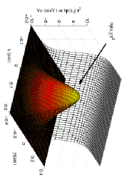
Figure 4: (color online) Schematic drawing of the probability density of a contact state on the $y$-edge. It overlaps with the entire region where the confining potential rises from $-V_{\rm gap}$ to $V_{\rm gap}$, so that it can inject/collect electrons of any Fermi energy from the Hall bar.

For the voltage probes (leads 2, 3, 5 and 6) we need a different strategy, since they are located on the $y=-L_{y}/2$, respectively $y=0$ edges of the Hall bar. The contact states are chosen to be of the form:

$$d^{\dagger}|{\rm vacuum}\rangle=\lambda\sum_{m}e^{-{(X_{m}-x_{c})^{2}\over a^{2}}+im\theta}\left|n,X_{m},\sigma\right>,$$ (13)

where $a$ is a parameter that controls the $x$ and $y$ extension of the wave-function, $\theta=0,\pi$ for $y=0,-L_{y}/2$ respectively, and $\lambda$ is the normalization factor. As $a$ changes, the shape of this wavefunction changes from a strip in the $x$-direction to a strip in the $y$-direction with fixed total area. We choose $a=0.2l$ so that the probability distribution of the contact states overlaps with the region of smooth variation of the confining potential near the $y$-edges. In this case, the profile of the contact states is an ellipse with its longer axis in the $y$-direction (see Fig. 4).

In Eq. (13), $x_{c}$ specifies the location of the contact state along the $y$-edge. We use $N_{c}/4$ ($25$, in these simulations) tight-binding chains for each of these leads, and correspondingly $N_{c}/4$ different contact states. For leads 3 and 5, the centers $x_{c}$ of their contact states are distributed uniformly in the range $[1,1.5]\mu$m, while for leads 2 and 6 the range is $[-1.5,-1]\mu$m. The summation in Eq. (13) is truncated so that no pair of neighboring contact states contain the same LL basis states in their expansions. The contact states on the $y=-L_{y}/2$ edge (for leads 2 and 3), are magnetic translations of the corresponding states of leads 5 and 6. The alternating phase factor $e^{im\pi}$ insures that contact states on different $y$-edges are orthogonal to one another, so that short-circuits are avoided.

III.3 Solving the scattering problem

The total Hamiltonian is the sum of the sample Hamiltonian, the Hamiltonians for the 6 leads, and the terms describing the contacts between sample and leads:

$${\cal H}={\cal H}_{\rm sample}+\sum_{\alpha=1}^{6}{\cal H}^{(\alpha)}_{\rm lead}+{\cal H}_{\rm contacts}$$ (14)

The numerical results presented here are obtained in the lowest Landau level (LLL) with $n=0$ (the spin projection is irrelevant. Calculations in higher LL proceed in a similar fashion). For simplicity, in the following we denote the LLL basis states by $|X_{j}\rangle=c_{j}^{\dagger}|{\rm vacuum}\rangle\equiv|n=0,X_{j},\sigma\rangle$. In the Hilbert subspace of the spin-polarized LLL, the Hamiltonian of the sample is:

$${\cal H}_{\rm sample}=\sum_{i=-N/2}^{N/2}\sum_{j=-N/2}^{N/2}\langle X_{i}|V_{c}+V_{d}|X_{j}\rangle\cdot c^{\dagger}_{i}c_{j}\;,$$ (15)

where $N=L_{x}L_{y}/(2\pi l^{2})$ is the number of states in a LL and an overall constant LLL energy shift $E_{0\sigma}$ has been ignored. The matrix elements $\langle X_{i}|V_{c}+V_{d}|X_{j}\rangle$ of the confining and disorder potentials are computed as described in Ref. Zhou04b, . Briefly, the idea is that matrix elements of a plane-wave are simple analytical functions:

$$\left<X_{i}\right|e^{i{\bf q\cdot r}}\left|X_{j}\right>=\delta_{X_{i},X_{j}-q_{y}l^{2}}e^{{i\over 2}q_{x}(X_{i}+X_{j})}e^{-{1\over 2}Q}$$

where $Q={1\over 2}l^{2}(q_{x}^{2}+q_{y}^{2})$. (The generalization for higher LLs and/or LL mixing is straightforward, see for instance Eq. (7) in Ref. Zhou04b, ). The strategy, then, is to perform a fast Fourier transform of the potentials on a grid dense enough to reproduce them with high accuracy while maintaining the sparseness of the Hamiltonian. The matrix element of each Fourier component is given by the previous formula, allowing one to efficiently compute the matrix elements of the confining and disorder potentials. Note that for higher LLs, the matrix elements differ only by a Laguerre polynomial. This is not likely to influence the physics in a significant way and suggests that numerical results for higher LLs should be qualitatively similar to those we present here for the LLL.

The leads are collections of $N_{c}^{\alpha}$ semi-infinite tight-binding chains, each describing a transverse channel:

$${\cal H}^{(\alpha)}_{\rm lead}=\sum_{i=1}^{N_{c}^{\alpha}}\sum_{m=0}^{\infty}\left[\epsilon_{0}c^{(\alpha)\dagger}_{i,m}c^{(\alpha)}_{i,m}-t\left(c^{(\alpha)\dagger}_{i,m}c^{(\alpha)}_{i,m+1}+h.c.\right)\right]$$ (16)

Thus, $c^{(\alpha)\dagger}_{i,m}$ creates an electron on the site $m\geq 0$ of the $i^{\rm th}$ transverse channel of lead $\alpha$. We use the convention that site $m=0$ is always the end site of the chain. The solution we present can be trivially generalized to allow for different $\epsilon_{0}$ and $t$ parameters for each channel, as well as longer-range hopping. However, since the physics in the sample is independent of the lead details (as long as the leads can carry currents to and from the sample) the simple choice we make should be sufficient. The choices for $t,\epsilon_{0}$ and number of channels $N_{c}^{\alpha}$ for each lead have been discussed previously.

Finally, the contacts are described by matrix elements between sites $m=0$ of the various channels and their corresponding contact states:

$${\cal H}_{\rm contacts}=-t\sum_{\alpha=1}^{6}\sum_{i=1}^{N_{c}^{\alpha}}\left[c^{(\alpha)\dagger}_{i,0}d^{(\alpha)}_{i}+h.c.\right]$$ (17)

where, as described in the previous section, each contact state is a linear combination of LLL basis states, which is localized in the appropriate region of the sample. Again, generalizations for more complex contacts can be easily incorporated, but should not be necessary.

We now have to solve a scattering problem for an electron injected with energy $E$ in the channel $j$ of lead $\beta$, which means that we must find an eigenstate ${\cal H}|\Psi_{\beta j}\rangle=E|\Psi_{\beta j}\rangle$ of the form

$$|\Psi_{\beta j}\rangle=\left[\sum_{\alpha=1}^{6}\sum_{i=1}^{N_{c}^{\alpha}}\sum_{m=0}^{\infty}\phi^{(\alpha)}_{i,m}c^{(\alpha)\dagger}_{i,m}+\sum_{j=-N/2}^{N/2}\phi_{j}c^{\dagger}_{j}\right]|{\rm vacuum}\rangle$$

where – with our convention for indexing channel sites – $\phi^{(\alpha)}_{i,m}=t_{\alpha i,\beta j}e^{ikm}+\delta_{ij}\delta_{\alpha\beta}e^{-ikm}$. In other words, there is an in-coming wave with unit amplitude in channel $(\beta j)$, and out-going waves with various transmission amplitudes in all other channels. The momentum $k>0$ is such that $E=\epsilon_{0}-2t\cos k$, i.e. it is the momentum of an electron with energy $E$ propagating on any of the tight-binding chains.

We solve this scattering problem by recasting it as a finite-size, inhomogeneous system of linear equations, which can be easily solved numerically. The unknowns are the amplitudes $\phi_{j}$ to find the electron in various LL states in the sample, plus 5 terms $\phi^{(\alpha)}_{i,m}$, $m=0,\dots,4$ for each channel (clearly, if one knows the wave-function at the first few sites of a tight-binding chain, one knows the wave-function along the entire chain). This solution is explained in detail in Ref. Zhou04b, , for two leads with multiple channels. The redistribution of the channels amongst more leads is trivial, since it only involves changing some of the matrix elements to the appropriate contact states.

The solution of this inhomogeneous system of linear equations, then, directly gives us the transmission coefficients $t_{\alpha i,\beta j}(E)$ from which we compute the conductance matrix [see Eq. (6)]. This is repeated for many Fermi energies $E_{F}$ corresponding to various filling factors $\nu$, to obtain the dependence $\hat{g}(\nu)$ of the various elements of the conductance matrix on the filling factor.

IV Numerical Results

IV.1 The conductance matrix for the LLL

Figure 5 shows numerical results for various matrix elements ${g}_{\alpha\beta}(\nu)$ inside the LLL $(0<\nu<1)$. The calculation is for the disorder potential shown in Fig. 3, for a magnetic field $B=3$T. Two facts are immediately apparent. First, for low filling factors ($\nu\leq 0.34$ for this disorder realization), the conductance matrix is symmetric to high accuracy, ${g}_{\alpha\beta}={g}_{\beta\alpha}$. From Eq. (7) it follows that $p_{\beta\rightarrow\alpha}=p_{\alpha\rightarrow\beta}$, i.e. the electron has the same (very small) probability to scatter in both directions. This is expected, since we know that at low filling factors, the states in the LLL are localized. Scattering from one terminal to another is only possible through tunneling of the electron from a state localized near one terminal, into a state localized near the other terminal. Such tunneling amplitudes are very small, explaining the small total probabilities for such scattering. Tunneling is also time-reversal symmetric – it happens with the same probability in both directions, consistent with the symmetry of the conductance matrix. These ideas will be made more precise in Section V, where we analyze the general structure allowed for the conductance matrix.

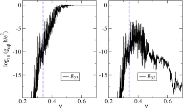
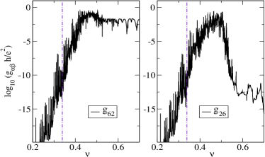
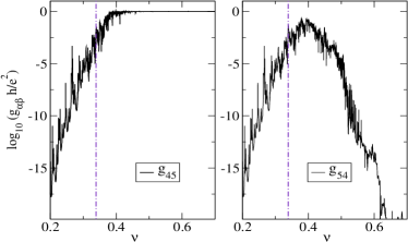
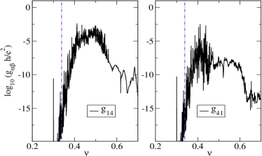
Figure 5: Representative conductance matrix elements, in units of $e^{2}/h$, as a function of $\nu$. The left panels show $g_{23}$, $g_{62}$, $g_{45}$, $g_{14}$, while the right panels show $g_{32}$, $g_{26}$, $g_{54}$, $g_{41}$. The top three left (right) panels characterize transport in (against) the direction of the edge currents. The bottom panels show the negligible direct transport between the current source and drain. For each pair, the traces are almost identical on the left, but very different on the right of the vertical line.

The second observation is that at high-filling factors $\nu\rightarrow 1$, we have $g_{\alpha,\alpha+1}\rightarrow e^{2}/h$ (where if $\alpha=6,\alpha+1=1$) while all other off-diagonal matrix elements become vanishingly small. In other words, an electron injected through terminal $\alpha+1$ scatters with unit probability into terminal $\alpha$. This behavior clearly signals the appearance of the edge states at higher filling factors. These are chiral states, carrying electrons only in the direction consistent with the orientation (sign of) the magnetic field $B$. These states are localized on the edges of the sample, on the “vertical walls” created by the confining potential.

Using Eq. (8), this shows that in the limit $\nu\rightarrow 1$, the conductance matrix converges to the simple form:

$$\hat{g}(\nu)\stackrel{{\scriptstyle\nu\rightarrow 1}}{{\longrightarrow}}\hat{g}^{(0)}={e^{2}\over h}\begin{pmatrix}-1&1&0&0&0&0\\ 0&-1&1&0&0&0\\ 0&0&-1&1&0&0\\ 0&0&0&-1&1&0\\ 0&0&0&0&-1&1\\ 1&0&0&0&0&-1\end{pmatrix}.$$ (18)

The resistances corresponding to this asymptotic limit are straightforward to find. Solving $\hat{I}_{14}=\hat{g}^{(0)}\cdot\hat{V}$ for $I=1,V_{4}=0$, we find $V_{5}=V_{6}=h/e^{2}$, $V_{2}=V_{3}=0$. Eqs. (4a), (4b) then give $R^{H}_{14,62}=R^{H}_{14,53}=h/e^{2}$, $R^{L}_{14,23}=R^{L}_{14,65}=0$. In other words, the values expected for the first IQHE plateau, which indeed is established when the LLL is more than half-filled.

IV.2 Fluctuations of resistances in the LLL

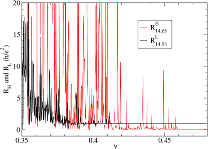
Figure 6: A pair of $R^{L}$ and $R^{H}$ for the disorder shown in Fig. (3 and $0<\nu<1$. $R^{L}$ shows strong fluctuation before quantization of $R^{H}$ is destroyed. The data are calculated at $T=0$.

The fluctuations of the various resistances are due to variations of $\hat{g}(\nu)$ from the asymptotic limit $\hat{g}^{(0)}$. Using $\hat{g}(\nu)$ shown in Fig. 5, we calculate the resistances for all filling factors $0<\nu<1$. In Fig. 6 we plot the pair $R^{H}_{14,65}$ and $R^{L}_{14,53}$ as a function of $\nu$ near half-filling. Three different regimes are apparent: for $\nu>0.46$, $R^{H}=h/e^{2}$ and $R^{L}=0$, corresponding to the first IQHE plateau. For $0.42<\nu<0.46$, $R^{L}$ exhibits large fluctuations, however $R^{H}$ is still well quantized. This is precisely the type of behavior observed experimentallyPeled et al. (2003a) (see Section II, point B). For $\nu<0.42$ the transition to the insulating phase occurs, and all resistances increase sharply as the wave-functions at the bottom of the LLL become more and more localized, leading to progressively smaller values for the matrix elements of $\hat{g}$ (see Fig. 5). This results in large fluctuations of both resistances at $T=0$; these are smeared out at finite $T$, as shown in Fig. 7.

Figure 7 shows all four resistances, for a different disorder realization, at $T=11.6$mK. The two Hall resistances are quantized to $h/e^{2}$ down to $\nu\approx 0.4$. Below $\nu\approx 0.46$, both $R^{L}$ exhibit fluctuations which quickly evolve into high peaks around $\nu=0.42$ where both $R^{H}$ still have only minor deviations from $h/e^{2}$. Comparing the upper and lower panel of Fig. 7, we see that the fluctuations of $R^{L}_{14,23}$ and $R^{L}_{14,65}$ are almost identical in this regime. Below $\nu\approx 0.4$ is the transition to the insulating phase.

The resistances in the insulating phase in Figs. 6 and 7 are not perfectly similar to the experimental results.Peled et al. (2003a) In the experiment, even at the lowest temperature, the rise in $R^{L}$ is less steep and less noisy than the behavior shown by our simulations. This is because when the Fermi energy resides amongst the low-$\nu$, strongly localized states of the LLL, the charge transport described here is no longer the dominant mechanism for conduction. Temperature assisted hopping conductivity and other inelastic scattering processes are likely to contribute to the conductance matrix more than the “band” conductance matrix which the simulation actually calculates. Therefore, we do not claim to have a realistic description of the insulating phase here. However, closer to half-filling the matrix elements of $\hat{g}$ become reasonably large, elastic scattering becomes the dominant mechanics for conduction and our simulations describe well the behavior observed experimentally.

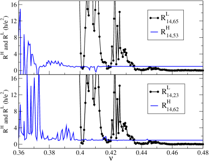
Figure 7: Both pairs of $R^{L}$ and $R^{H}$ for a different disorder. Both $R^{L}$ show strong fluctuations before the quantization of the $R^{H}$ disappears. The results correspond to $T=11.6$mK.

IV.3 The conductance matrix of higher LL

The conductance matrix when the Fermi level is in a higher LL can be obtained from the conductance matrix of the LLL using the superposition principle.Shahar et al. (1997) We simply add a contribution $\hat{g}^{(0)}$ for each completely filled LL to the matrix $\hat{g}(\nu)$ describing the response of the LL hosting the Fermi energy (in this context, $0<\nu<1$ denotes the filling factor of the LL hosting the Fermi energy, not the total filling factor). As discussed, $\hat{g}^{(0)}$ describes transport through the edge states, which is the only possible contribution of a completely filled LL. Indeed, we see that if $E_{F}$ is such that $n$ LL are completely filled, according to the superposition principle we have $\hat{g}=n\hat{g}^{(0)}$. This immediately leads to the solutions $R^{H}=h/(ne^{2})$, $R^{L}=0$, i.e. the $n^{\rm th}$ IQHE plateau, as expected.

The validity of the superposition principle (which we take for granted here), is based on the belief that the IQHE transition can be described within one single LL, and that each plateau-to-plateau transition is in the same universality class. Wei et al.Wei et al. (1988) experimentally confirmed this hypothesis. Shahar et al.Shahar et al. (1997) further developed this idea by mapping the transition between adjacent IQHE plateaus to the insulator-to-QH transition in the LLL.

The superposition principle relies on several conditions, which are satisfied in our simulations: (1) One must confirm that for a single LL, as the Fermi energy is raised and $\nu\rightarrow 1$, the conductance matrix $\hat{g}\rightarrow\hat{g}^{(0)}$ at reasonable filling factors, close to the center of the LL. We have already shown that our simulations satisfy this for the LLL. Higher LL should behave similarly, since the only difference is a simple change in the matrix elements of the disorder plus confining potential [see Eq. (15) and discussion following it]. (2) The cyclotron gap is large enough to justify neglect of the LL mixing. This is certainly valid for $\nu\sim n+0.5$, because here the charge transport is dominated by processes in the bulk of the Hall bar, where the disorder is much smaller than the cyclotron gap. However, for the spatially close edge-states of different LLs, one does expect inter-Landau level and spin-dependent scattering to become relevant.note As a result, we do not claim that the edge-states produced in the single LL simulation are necessarily realistic. However, this has no influence on the conductance matrix. The reason is simple: there is no backscattering among the edge-states.(Büttiker, 1988) All edge-states near the same boundary of the sample carry currents in the same direction, irrespective of their LL index and spin-polarization. Scattering among these edge-states results in a unitary transformation which conserves the total probability to carry electrons from one terminal to the next. As a result, even though inclusion of the filled LL states in the simulation may change some details of the edge-state wave-functions, the total conduction matrix $\hat{g}$ is not affected. This, in conjunction with the significant economy of CPU time when LL mixing is neglected, explains why we perform the simulations for a single LL.

IV.4 Fluctuations of resistances in higher LL

Using the superposition principle, the fluctuations of the resistances for $1<\nu<2$ can be calculated using the conductance matrix $\hat{g}(\nu-1)+\hat{g}^{(0)}$, where $\hat{g}(\nu)$ is the LLL conductance matrix already analyzed and the second term is the contribution of the filled LL.

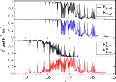
Figure 8: A typical transition from the first to the second IQHE plateau at $T=0$. Lower panel: $R^{L}_{14,62}$ and $R^{H}_{14,23}$ in units of $h/e^{2}$. Upper panel: The sum $R^{L}_{14,62}+R^{H}_{14,23}=R_{14,63}$ of the resistances shown in the lower panel, and $R_{2t}=R_{63,63}$ (shifted by $-0.5{h/e^{2}}$). Vertical lines indicate the boundaries of the critical region. See text for more details.

The resistances $R^{H}_{14,62}$ and $R^{L}_{14,23}$ corresponding to the disorder shown in Fig. 3 are plotted in the lower panel of Fig. 8. The three regimes found experimentally (see Sec. II, points A1 – A3) are clearly observed within the transition from the first to the second IQHE plateau. Their (approximate) boundaries are marked by vertical lines in Fig. 8, as a guide to the eye. At low-$\nu$ (high-$B$), the fluctuations of $R^{H}$ and $R^{L}$ are correlated such that $R^{L}+R^{H}=h/e^{2}$. This is seen more clearly in the upper panel, where their sum $R^{H}_{14,62}+R^{L}_{14,23}=R_{14,63}$ is plotted. At high-$\nu$ (low-$B$) $R^{H}={h/(2e^{2})}$ is quantized while $R^{L}$ exhibits strong fluctuations. In the intermediate regime, both $R^{H}$ and $R^{L}$ have strong, uncorrelated fluctuations. The upper panel of Fig. 8 compares $R^{L}+R^{H}$ with $R_{2t}$ ($R_{2t}$ is shifted by $0.5h/e^{2}$). As found experimentally,(Peled et al., 2003b) (Sec. II, point C) the two curves are almost identical. Only minor differences at high-$\nu$ are visible.

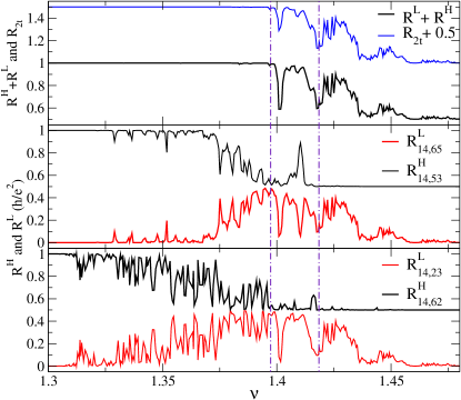
Figure 9: The result of a simulation performed at $T=11.6$mK. (a) Comparison between $R_{2t}$ and $R^{H}+R^{L}$. Here, $R_{2t}$ has been shifted up for clarity. (b), (c) the two pairs of $R^{L}$ and $R^{H}$ for $1<\nu<2$. The vertical lines indicate the boundary of three distinctive fluctuation regimes.

Figure 9 shows a set of data calculated for $T=11.6$ mK with a different disorder realization. Both pairs of resistances are shown (the lower panels). The thermal average was performed using Eq. (9). At finite $T$, the traces are much smoother than at $T=0$. The scale of the fluctuations in Fig. 9 is comparable to that of the experimental data in Ref. Peled et al., 2003b – an indication that our simulations provide a good approximation of the experimental conditions. While the fluctuation patterns are clearly sample (disorder) specific, the three distinct fluctuation regimes are again clearly seen. The comparison between $R_{2t}$ and $R_{14,63}$ (upper panel) shows that they are approximately equal over the entire transition. Moreover, it is also apparent that the two pairs of $R^{H}$ and $R^{L}$ have different fluctuation patterns, except on the high-$\nu$ side where the two $R^{L}$ are almost identical. Another observation in all our simulations is that everywhere during this $1<\nu<2$ transition, $0\leq R^{L}\leq 0.5h/e^{2}$ and $0.5h/e^{2}<R^{H}<h/e^{2}$. Within experimental error bars, the experimental resistance traces also stay within these limits.Peled et al. (2003b) Thus, all observations are in agreement with the experimental facts.

V Generalized Landauer-Büttiker model

So far, we have shown that our numerical simulations faithfully reproduce the experimental results. In this section we explain the physics underlying these various types of correlations, using a simple but very general model. The consequences of changing the orientation of the magnetic field, $B\rightarrow-B$, are also addressed.

Since all resistances are functions of the various conductance matrix elements, it is clear that the correlations of the various resistances are encoded in the structure of the conductance matrix $\hat{g}$. Thus, it is important to understand the allowed structure of the conduction matrix, based on the various constraints it must satisfy, and the physics known to be relevant for transport in a LL.

As already discussed, the conductance matrix in the presence of $n$ filled LLs is of the form $n\hat{g}^{(0)}+\hat{g}(\nu-n)$, where the first part is the edge-state contribution of the filled LL levels, and the second term is the contribution of the LL hosting the Fermi energy. The challenge, then, is to understand $\hat{g}(\nu)$. Its matrix elements satisfy the following general constraints: (i) since they are proportional to transmission probabilities, all off-diagonal matrix elements are positive numbers $g_{\alpha,\beta\neq\alpha}\geq 0$ [see Eq. (7)]; (ii) Let $N_{T}\geq 2$ be the number of terminals ($N_{T}=6$ is the case of interest to us). The $N_{T}(N_{T}-1)$ off-diagonal matrix elements must satisfy the $2N_{T}$ constraints of Eq. (8). Half of them fix the value of the diagonal matrix elements, leaving a total of $N_{T}-1$ supplementary constraints for the off-diagonal elements (one constraint is trivially satisfied if the other $2N_{T}-1$ hold).

If $N_{T}=2$, this implies immediately that the conductance matrix must be symmetric, i.e. the most general possible form is:

$$\hat{g}_{2}=G\left(\begin{array}[c]{cc}-1&1\\ 1&-1\\ \end{array}\right)$$ (19)

$G$ is the total conductance between the two terminals, since in this geometry we must have $I_{1}=-I_{2}=-I$ (all the current injected through one terminal must be removed through the other terminal), and therefore

$$\left(\begin{array}[c]{c}I_{1}\\ I_{2}\\ \end{array}\right)=\hat{g}_{2}\cdot\left(\begin{array}[c]{c}V_{1}\\ V_{2}\\ \end{array}\right)\rightarrow I=G(V_{1}-V_{2})$$

For $N_{T}=3$, the situation is more interesting. First, we separate the “symmetric” contributions. Let us denote

$$G_{\alpha\beta}=\min\left(g_{\alpha\beta},g_{\beta\alpha}\right)$$

We can then rewrite:

$$\hat{g}_{3}=G_{12}\left(\begin{array}[c]{ccc}-1&1&0\\ 1&-1&0\\ 0&0&0\\ \end{array}\right)+G_{13}\left(\begin{array}[c]{ccc}-1&0&1\\ 0&0&0\\ 1&0&-1\\ \end{array}\right)$$

$$+G_{23}\left(\begin{array}[c]{ccc}0&0&0\\ 0&-1&1\\ 0&1&-1\\ \end{array}\right)+\Delta\hat{g}_{3}$$

If the system is time-reversal symmetric, then $\Delta\hat{g}_{3}=0$ since transport must proceed with equal probability in any two opposite directions, $p_{\alpha\rightarrow\beta}=p_{\beta\rightarrow\alpha}$. However, in the presence of a magnetic field, there is a preferred direction of charge transport chosen by the magnetic field. Thus, in cases of interest to us the conductance matrix is generally not symmetric (as already exemplified by $\hat{g}^{(0)}$).

The matrix $\Delta\hat{g}_{3}$ which contains the non-symmetric contributions must still satisfy the constraints of Eq. (8), since the symmetric contributions do. Moreover, by construction, exactly 3 of its 6 off-diagonal matrix elements are zero. The remaining (positive) matrix elements must be all equal, and such that there is one on each row and on each column, otherwise the constraints cannot be satisfied. The only possibilities are either

$$\Delta\hat{g}_{3}=c\left(\begin{array}[c]{ccc}-1&1&0\\ 0&-1&1\\ 1&0&-1\\ \end{array}\right)\mbox{ or }\Delta\hat{g}_{3}=c\left(\begin{array}[c]{ccc}-1&0&1\\ 1&-1&0\\ 0&1&-1\\ \end{array}\right)$$

where $c>0$ is a constant. We call such contributions, which involve a closed loop of at least three terminals (here, $1\rightarrow 2\rightarrow 3$ or $1\rightarrow 3\rightarrow 2$ ) in an order selected by the magnetic field orientation, a “chiral” contribution.

This approach can be straightforwardly generalized to $N_{T}>3$. In cases with broken time-reversal symmetry, we expect to have some symmetric and some chiral contributions. To be more precise, we define the matrix

$$l(a,b)|_{\alpha\beta}=\delta_{\alpha a}\delta_{\beta b}-\frac{1}{2}\delta_{\alpha a}\delta_{\beta a}-\frac{1}{2}\delta_{\alpha b}\delta_{\beta b}$$ (20)

which contributes a unit to the off-diagonal element $g_{ab}$. For any ordered sequence of terminals $a_{1},a_{2},...,a_{n}$, we define the matrix:

$$\hat{r}(a_{1},\cdots,a_{n})=\hat{l}(a_{1},a_{2})+\hat{l}(a_{2},a_{3})+\dots+\hat{l}(a_{n},a_{1}).$$ (21)

Any such $\hat{r}$ matrix satisfies all the constraints of Eq. (8). With this notation, and assuming that the magnetic field is such as to select the first form of $\Delta\hat{g}_{3}$, we can rewrite:

$$\hat{g}_{3}=G_{12}\hat{r}(1,2)+G_{13}\hat{r}(1,3)+G_{23}\hat{r}(2,3)+c\hat{r}(1,2,3)$$ (22)

Any $N_{T}\times N_{T}$ conductance matrix $\hat{g}$ can be decomposed in a similar fashion, into a sum of symmetric (“resistances”) and chiral contributions:

$$\hat{g}=\sum c_{a_{1},\cdots,a_{n}}\hat{r}(a_{1},\cdots,a_{n}).$$ (23)

where $c_{a_{1},\cdots,a_{n}}$ are positive numbers. The symmetric part is simply $\sum_{a<b}G_{ab}\hat{r}(a,b)$, where $G_{ab}=\min(g_{ab},g_{ba})$. This leaves at most $N_{T}(N_{T}-1)/2$ finite, positive off-diagonal matrix elements, which can be grouped into a sum of “chiral” contributions. To do this, start with the smallest non-zero matrix element left, say $g_{ab}-G_{ab}$, then draw a loop $a\rightarrow a_{1}\rightarrow\dots\rightarrow a_{n}\rightarrow b$ with bonds only connecting pairs of contacts sharing non-zero matrix elements. We can now separate a contribution $(g_{ab}-G_{ab})\hat{r}(a,a_{1},...,a_{n},b)$, insuring that the number of zero off-diagonal matrix elements of the remaining matrix has increased by at least one, while all the finite off-diagonal matrix elements are still positive. The procedure is repeated until the decomposition is completed.

V.1 Six-terminal geometry for the IQHE

While the decomposition of Eq. (23) is very general, which of the decomposition terms are important depends, of course, on the physical system considered. We now return to the problem of interest to us, namely the $6\times 6$ matrix $\hat{g}(\nu)$ describing the contribution to the total conductance of the LL hosting the Fermi energy. From now, $0<\nu<1$ stands for the filling factor of the LL hosting the Fermi energy. The total filling factor is $n+\nu$, where $n$ is the number of filled LLs.

At low-$\nu$, all states of the LL hosting $E_{F}$ are localized and transport can only occur through tunneling. Tunneling occurs with equal probability in both directions. Thus, on very general grounds, here we expect the conductance matrix to be symmetric, with small off-diagonal elements since tunneling probabilities are small.

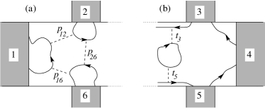
Figure 10: A semi-classical illustration of possible transport between terminals, for (a) low filling factors $\nu\rightarrow 0$. In this case, all states in the LL hosting the Fermi level are localized, and transport can only occur by tunneling. (b) at high filling factors $\nu\rightarrow 1$, the edge states are established and dominate the transport. Jain-Kivelson tunneling through localized states inside the sample can create short chiral currents.

Let us consider this case in more detail. In Fig. 10(a), we sketch some possible routes for charge transport between three terminals, at low-$\nu$. The wave-functions are drawn in a semi-classical manner, following equipotentials of the disorder potential in the direction determined by the sign of $B$. This does not mean that our arguments only hold in the semi-classical regime. They are general and hold in the quantum regime – we just do not know how to draw quantum mechanical wave-functions.

Most of the electrons injected through any of the terminals will be scattered back. However, with a small probability $p_{12}$, electrons injected from terminal 2 can tunnel to near terminal 1. Another possible route of scattering from 2 into 1, is for electrons to first tunnel to a state near 6 (probability $p_{26}$) and from there to near 1 (probability $p_{16}$). The total probability for this process is $(1-p_{12})p_{26}p_{61}(1-p_{12})$. The electron can, however, make any number of closed loops between finally entering in 1, and so the total probability to arrive from 2 to 1 is

$$p_{2\rightarrow 1}=p_{12}+\frac{(1-p_{12})p_{26}p_{61}(1-p_{12})}{1-p_{12}p_{26}p_{61}}$$

Similarly, an electron injected through 1 can scatter into 2 either directly [with probability $(1-p_{16})p_{12}(1-p_{26})$] or can make any number of loops, yielding

$$p_{1\rightarrow 2}=\frac{(1-p_{16})p_{12}(1-p_{26})}{1-p_{12}p_{26}p_{61}}$$

The other probabilities $p_{1\rightarrow 6},p_{6\rightarrow 1},p_{2\rightarrow 6}$ and $p_{6\rightarrow 2}$ can be calculated similarly.

Using $G_{ab}=\frac{e^{2}}{h}\min(p_{a\rightarrow b},p_{b\rightarrow a})>0$, we find $G_{\alpha\beta}=\frac{e^{2}}{h}p_{\alpha\beta}+O(p^{3})$, i.e. indeed, the largest contribution to transport between these 3 terminals comes from direct tunneling and is symmetric. However, the conductance matrix is not fully symmetric, since $p_{2\rightarrow 1}-p_{1\rightarrow 2}>0$. In fact, one finds that $p_{2\rightarrow 1}-p_{1\rightarrow 2}=p_{6\rightarrow 2}-p_{2\rightarrow 6}=p_{1\rightarrow 6}-p_{6\rightarrow 1}=c=p_{12}p_{26}+p_{12}p_{16}+p_{26}p_{61}+O(p^{3})$, showing also the appearance of a very small chiral contribution. Thus, the contribution of these processes to the conductance matrix is precisely of the expected form of Eq. (22). This derivation completely ignores interference effects between different scattering paths, and therefore is valid only in the presence of significant dephasing. Our numerical simulations, on the other hand, assume full coherence between all electron wave-functions (there is no inelastic scattering in our Hamiltonian). In such a case, one should sum the amplitudes of probabilities for various processes, and then square its modulus to find the total probability. The derivation for this case is very similar to the above one (also see Ref. Zhou04c, ). The main contribution to the off-diagonal conductance matrix elements are still due to the direct tunneling, e.g. $G_{12}=\frac{e^{2}}{h}|t_{12}|^{2}$, where $t_{12}$ is the amplitude of probability to tunnel from 1 to 2 (so that $|t_{12}|^{2}=p_{12}$). The difference is that the chiral current is now of order $|t|^{3}$, not $p^{2}=|t|^{4}$ as when the interference is ignored. The reality is in between, since in the real samples there is some amount of decoherence. Irrespective of how much decoherence there is, a predominantly symmetric conductance matrix is inevitable if tunneling is the only means of charge transport.

Of course, in order to derive an expression for the entire $6\times 6$ conductance matrix, we have to also consider tunneling to the other 3 terminals in all possible combinations. It should be apparent that as long as all $p\ll 1$, the only effect of that is to add symmetric terms of order $p$ between all pairs of terminals connected by direct tunneling, and much smaller chiral terms, of order $p^{2}$ or $|t|^{3}$, for various closed loops. This explains why for low-$\nu$, $\hat{g}$ is symmetric with small off-diagonal components, as indeed confirmed by the numerical simulations (see Fig. 5).

At high-$\nu$, on the other hand, the transport mechanism is very different. As expected on general grounds (and confirmed by the numerics) edge states are established within the LL once $\nu>0.5$. With very high probability, electrons are transported through the edge states to the next terminal $\alpha+1\rightarrow\alpha$. In the limit $\nu\rightarrow 1$ we expect and find $\hat{g}\rightarrow\frac{e^{2}}{h}\hat{r}(1,2,3,4,5,6)=\hat{g}^{(0)}$.

For intermediate $\nu$, however, shorter chiral loops containing edge states can be established through tunneling, as sketched in Fig. 10(b). Assume that an electron leaving contact 3 can tunnel with amplitudes of probability $t_{3}$ and $t_{5}$ to and out of a localized state inside the sample, to join the opposite edge state and enter 5. This is precisely the Jain-Kivelson phenomenology.Jain and Kivelson (1988) Summing over all possible processes and ignoring decoherence, we find their resultJain and Kivelson (1988)

$$p_{3\rightarrow 5}=\frac{h}{e^{2}}g_{53}=\left|\frac{t_{3}t_{5}}{1-r_{3}r_{5}\exp(i\phi/\phi_{0})}\right|^{2}$$ (24)

where $\phi$ is the flux enclosed by the localized state, $\phi_{0}=h/e$ is the unit of flux, and $|r_{3}|=\sqrt{1-|t_{3}|^{2}},|r_{5}|=\sqrt{1-|t_{5}|^{2}}$ are the amplitudes to avoid the corresponding tunneling. On the other hand, $p_{5\rightarrow 3}=0$, since in this scenario, no electron leaving 5 enters 3. Thus, in this case there is no symmetric term proportional to $\hat{r}(3,5)$, only a chiral loop term $g_{53}\hat{r}(3,4,5)$. Physically, this term represents the backscattered current of the Jain-Kivelson model.Jain and Kivelson (1988) Other shorter chiral loops can be established by tunneling between other pairs of edge states, so in the high-$\nu$ limit we expect the conductance matrix to be a sum of such chiral loops. Again, inclusion of partial or total dephasing does not change this conclusion.

This analysis has reconfirmed our assertion that the conductance matrix can be decomposed into a sum of symmetric terms and chiral terms. For this particular system, we have now shown that at low-$\nu$, the symmetric terms are the dominant (although small) contribution, while at high-$\nu$, chiral loops are the dominant contribution. Near half-filling, we expect both types of terms to be important. Consider then the general form:

$$\hat{g} = n\hat{g}^{(0)}+G_{12}\hat{r}(1,2)+G_{16}\hat{r}(1,6)+G_{26}\hat{r}(2,6)+G_{34}\hat{r}(3,4)+G_{35}\hat{r}(3,5)+G_{45}\hat{r}(4,5)+$$ (25)

$$+\frac{e^{2}}{h}\left[c_{0}\hat{g}^{(0)}+c_{1}\hat{r}(1,2,6)+c_{2}\hat{r}(2,3,5,6)+c_{3}\hat{r}(3,4,5)+c_{4}\hat{r}(1,2,3,5,6)+c_{5}\hat{r}(2,3,4,5,6)\right].$$

The first term is the contribution of the $n$ completely filled lower LLs, while all other terms describe transport in the LL hosting $E_{F}$. Eq. (25) is not the most general possible decomposition – that would have 15 symmetric and 10 chiral terms. In Eq. (25) we assume no tunneling (no symmetric terms) between the left and right sides of the sample. The largest such neglected terms are $G_{23}\hat{r}(2,3)$ and $G_{56}\hat{r}(5,6)$. Numerically, we find $G_{23},G_{56}<10^{-4}\frac{e^{2}}{h}$ [see Fig. 5, where $G_{23}=\min(g_{23},g_{32})$, etc.]. We analyze the influence of these neglected terms on the resistance fluctuations in the next section. The 4 chiral loops neglected all have one “diagonal” link between 2 and 5, or between 3 and 6. As explained, chiral loops are important at larger filling factors, because of Jain-Kivelson scattering between opposite edge states. Such scattering does not mediate direct transport between $2\leftrightarrow 5$ or $3\leftrightarrow 6$ (see discussion below), so these terms can be safely neglected.

The model of Eq. (25) is thus a parameterization of the 6$\times 6$ matrix $\hat{g}$ with 12 independent parameters. At low $\nu$, the chiral terms $c_{i}\rightarrow 0$ and the decomposition is dominated by the symmetric terms. At high $\nu$, the symmetric terms vanish $G_{\alpha\beta}\rightarrow 0$ while the chiral terms are important, in particular $c_{0}\rightarrow 1$. Near half-filling, all terms are likely to contribute. Eq. (25) thus covers all possible filling factors $0<\nu<1$. Figure 11 sketches the elements contained in this model. The closed directed loops indicate chiral terms while the resistors indicate the existence of symmetric terms. Resistors suggest dissipation; as we show shortly, they play a role only during transitions between QHE plateaus. Close to integer filling, where the Hall conductances are quantized and the sample is disipationless, $\hat{g}\rightarrow n\hat{g}^{(0)}$ and all symmetric (“resistors”) terms vanish, as do the shorter chiral loops.

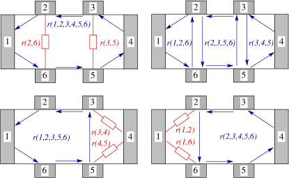
Figure 11: Terms contained in the general decomposition of Eq. (25). Symmetric terms are represented as resistors, while chiral terms are represented as closed directed loops.

V.2 The correlations of the resistance fluctuations

With Eq. (25), the equations $\hat{I}_{14}=\hat{g}\cdot\hat{V}$ and $\hat{I}_{63}=\hat{g}\cdot\hat{V^{\prime}}$ can be solved analytically and the various Hall, longitudinal and two-terminal resistances can be calculated in terms of these 12 parameters. The complete solutions are very long and we do not list them here.

The following identity is found to hold:

$$R_{14,63}=R_{63,63}=\frac{h}{e^{2}}\frac{1}{n+c_{0}+c_{2}+c_{4}+c_{5}}.$$ (26)

Since $R_{63,63}=R_{2t}$, whereas $R_{14,63}=R^{H}_{14,62}+R^{L}_{14,23}=R^{L}_{14,65}+R^{H}_{14,53}$, this means that $R_{2t}=R^{H}+R^{L}$ irrespective of the value of the 12 parameters. In other words, this identity is obeyed for all $\nu$, which explains why it is observed in both experiment and simulation. (This identity is not observed in experiment for low magnetic fields. This can be ascribed to deviations from the IQHE regime, where some of the approximations we make here – ignoring the LL mixing, for example – fail.)

In Eq. (26), $n+c_{0}+c_{2}+c_{4}+c_{5}$ is the total chiral current flowing along the $6\rightarrow 5$ and $3\rightarrow 2$ edges. As discussed, at low-$\nu$ the chiral currents in the LL hosting $E_{F}$ are vanishingly small: $c_{i}=0$, $i=1,...,6$ (there are no edge states established yet, and tunneling contributions to chiral currents are of order $t^{3}$ or less, as showed in the previous section. Below $\nu_{c}$, all $t<10^{-2}$, see Fig. 5). It follows that at low-$\nu$, $R^{L}+R^{H}=h/(ne^{2})$, explaining the perfect correlations in the fluctuation patterns of the two resistances, seen experimentally and numerically.

In the high-$\nu$ regime the transport is dominated by the chiral currents created by tunneling between opposite edge states, through localized states inside the sample.Jain and Kivelson (1988) The most general possible situation is sketched in Fig. 12. $p_{1}$, $p_{2}$, and $p_{3}$ are the total probabilities for tunneling between the pairs of edges, summing over all the possible tunneling processes through all available localized states in the sample. Each such contribution fluctuates strongly as $B$ (or $\nu$) is changed, since the magnetic flux enclosed by various localized states changes significantly [see Eq. (24) for the simplest possible expression for such a probability]. The various conductance matrix elements can be simply read off this figure; for example, $\frac{h}{e^{2}}g_{12}=p_{2\rightarrow 1}=1-p_{1}$. After adding the contribution of the $n$ filled LL, the total conductance matrix can be written as a sum of chiral terms, consistent with Eq. (25):

$$\hat{g}=(1-p_{1}-p_{2}-p_{3})\hat{g}^{(0)}+\frac{e^{2}}{h}p_{2}\left[\hat{r}(1,2,6)+\hat{r}(3,4,5)\right]$$ (27)

$$+\frac{e^{2}}{h}\left[p_{3}\hat{r}(1,2,3,5,6)+p_{1}\hat{r}(2,3,4,5,6)\right]+n\hat{g}^{(0)}.$$

In this case, the equation $\hat{I}_{14}=\hat{g}\cdot\hat{V}$ is trivial to solve. We find:

$$R^{H}_{14,62}=R^{H}_{14,53}=\frac{h}{(n+1)e^{2}},$$

i.e. the Hall resistances are precisely quantized, whereas

$$R^{L}_{14,23}=R^{L}_{14,65}=\frac{h}{(n+1)e^{2}}\cdot\frac{p_{2}}{n+1-p_{2}}.$$

Note that the result only depends on $p_{2}$, i.e. on tunneling between edge states in the central part of the device, between the 4 voltage terminals. This is further justification that a short sample is sufficient for the numerical simulation. Since $p_{2}$ has a strong resonant dependence on $E_{F}$ (or $\nu$), it follows that the two $R^{L}$ fluctuate strongly, but with identical patterns. This is precisely what is observed in experiment and numerics, on the high-$\nu$ side of the transition (see Figs. 7 and 9) and supports our assertion that the fluctuations in this regime are caused by Jain-Kivelson tunneling. In particular, if $n=0$ (transition inside the spin-up LLL), $R^{L}$ can be arbitrarily large when $p_{2}\rightarrow 1$ (see Fig. 7). In higher LLs, the amplitude of fluctuations of $R^{L}$ is $h/[n(n+1)]e^{2}$ or less, as observed both experimentally and in our simulations (see Fig. 9).

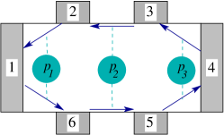
Figure 12: Possible Jain-Kivelson processes in the sample for high-$\nu$ region.

These results are very interesting because they show that one does not actually need to know the conductance matrix in order to understand what correlations might exist between various resistances. All that is needed is to have some idea of its general structure, which can be inferred based on physical arguments. At low $\nu$ the conductance matrix is the sum between $n\hat{g}^{(0)}$ and a symmetric matrix describing tunneling between various terminals (ignoring tunneling between the left and right sides, for the time being). The solutions of $\hat{I}_{14}=\hat{g}\cdot\hat{V}$ for such a matrix always satisfy $R^{L}+R^{H}=h/(ne^{2})$, no matter what are the off-diagonal values of the symmetric component. It follows that this identity must be obeyed in experiments as long as the conductance matrix has this form, i.e. for filling factors low-enough that tunneling is the dominant transport mechanism in the LL hosting $E_{F}$. On the other hand, for high filling factors, physical arguments based on the appearance of the edge states and the Jain-Kivelson phenomenology lead to the conclusion that the general form of the conductance matrix is like in Eq. (27). In this case, we find that irrespective of the values of the parameters $p_{1},p_{2}$ and $p_{3}$, the $R^{H}$ are quantized while the two $R^{L}$ fluctuate with identical patterns. Finally, to cover all possible $\nu$, we must include in $\hat{g}$ both types of allowed symmetric and chiral terms. In this case, we find that the identity $R_{2t}=R^{H}+R^{L}$ holds, irrespective of the values of the various parameters. Such arguments can be straightforwardly generalized to geometries with any number of terminals, allowing one to easily test in what cases are correlations expected on such general grounds. The behavior when the sign of $B$ is changed can also be understood easily, as we show now.

V.3 Changing the orientation of the magnetic field

If $B$ changes sign, the Onsager reciprocal relation(Baranger and Stone, 1989) reads

$$\hat{g}(-B)=[\hat{g}(B)]^{T}.$$

That this must be so is obvious for our generic conductance matrix of Eq. (25): the time-reversal symmetric tunneling is not affected by this sign change, but the flow of the chiral currents is reversed (equivalent with taking the transpose). The solutions of $\hat{I}_{14}=\hat{g}(-B)\cdot\hat{v}$ are then related to the solutions of $\hat{I}_{14}=\hat{g}(B)\cdot\hat{V}$ by $v_{2}=V_{6}$, $v_{3}=V_{5}$, $v_{5}=V_{3}$ and $v_{6}=V_{2}$, provided that the same index exchanges $2\leftrightarrow 6$, $3\leftrightarrow 5$, are performed for all $G_{ab}$. Terms not invariant under this transformation are $G_{12}$, $G_{16}$, $G_{43}$, and $G_{45}$. In the experimental setup, these four terms must be very small, due to the long distance between source and drain, and their nearby contacts. (In the simulation, these terms are sometimes not negligible because the simulated sample is rather short). If we set these 4 terms to zero and keep only the largest symmetric terms $G_{26}$ and $G_{35}$ in Eq. (25), we find that $R^{L}_{14,23}(B)=R^{L}_{14,65}(-B)$ and vice versa. In other words, the fluctuation pattern of one $R^{L}$ mirrors that of the other $R^{L}$ when $B\rightarrow-B$, as observed experimentally.Peled04 Small violations of this symmetry observed experimentally at low-$\nu$, are likely due to the perturbative corrections from the very small, non-invariant tunneling contributions proportional to $G_{12}-G_{16}$ and $G_{43}-G_{45}$. This is confirmed in the next section.

V.4 Small corrections to correlations and symmetry

The most significant terms neglected in the general decomposition of Eq. (25) are $G_{23}\hat{r}(2,3)$ and $G_{56}\hat{r}(5,6)$, which are due to tunneling between the neighboring voltage probes. All other tunneling terms neglected are smaller than these, because they are between contacts further apart. Remember that even these two terms are very small; numerically we found that they are of order $10^{-4}\frac{e^{2}}{h}$ or less (see Fig. 5). We now investigate whether the inclusion of these terms violates significantly the various correlations established in their absence. For simplicity, in the rest of this section we set $e^{2}/h=1$, in other words we measure all conductances in $e^{2}/h$ units.

We first investigate the effects of adding the $G_{23}$ and $G_{56}$ terms on the low-$\nu$ correlations $R^{H}+R^{L}=1/n$. We set all $c_{i}=0$, since at low-$\nu$ the chiral terms are negligible compared to the symmetric terms. To first order perturbation in $G_{23}$ and $G_{56}$, we find:

$$R_{14,63}-\frac{1}{n}={[n(G_{26}+G_{12})+F_{1}]G_{23}\over n^{2}[nF_{2}+F_{1}]}$$

$$+{[n(G_{35}+G_{45})+F_{3}]G_{56}\over n^{2}[nF_{4}+F_{3}]}+\cdots,$$ (28)

where

$$F_{1}=G_{16}G_{26}+G_{12}G_{16}+G_{12}G_{26},\;F_{2}=G_{16}+G_{26}+G_{12},$$

$$F_{3}=G_{34}G_{45}+G_{34}G_{35}+G_{35}G_{45},\;F_{4}=G_{34}+G_{35}+G_{45}.$$

In the given experimental geometry, we expect that $G_{12},G_{16}\ll G_{26}$ and $G_{34},G_{45}\ll G_{35}$, since terminals 1 and 4 are very far from 2 and 3, respectively 5 and 6, and thus the tunneling probabilities must be much smaller. Within this limit, the previous expression can be further simplified to:

$$R_{14,63}-\frac{1}{n}\approx\frac{G_{23}+G_{56}}{n^{3}}$$

In other words, the identity $R^{H}+R^{L}=R_{14,63}=1/n$ should indeed be obeyed with high accuracy, as long as the direct tunneling between 2 and 3, respectively 5 and 6, as well as the chiral contributions, are indeed small.

We now consider the effect of adding the $G_{23}$ and $G_{56}$ terms on the identity $R^{L}+R^{H}=R_{2t}$. After expanding to first order in these two quantities, we find:

$$R_{14,63}-R_{63,63}=-{G_{45}G_{56}\over A_{1}}-{G_{12}G_{23}\over A_{2}}+\cdots.$$ (29)

where we define $C_{T}=\sum_{i=0}^{5}c_{i}$ and

$$A_{1}=(n+C_{T}-c_{1}+G_{35})(n+C_{T}-c_{1}-c_{3})(n+c_{0}+c_{3}+c_{5})$$

$$A_{2}=(n+C_{T}-c_{3}+G_{26})(n+C_{T}-c_{1}-c_{3})(n+c_{0}+c_{1}+c_{4})$$

Since $G_{45}$, $G_{56}$, $G_{12}$, and $G_{23}$ are all small numbers, we have $A_{1},A_{2}\sim n^{3}\geq 1$, and therefore this correction is also small for all values of $\nu$.

Finally, we investigate how the $B$-reversal symmetry is perturbed by a small imbalance between $G_{34}$ and $G_{45}$, respectively $G_{12}$ and $G_{16}$. As stated before, $R^{H}(-B)$ and $R^{L}(-B)$ are calculated with $\hat{g}^{T}$. For simplicity, here we take $G_{23}=G_{56}=0$, and find:

$$R^{L}_{14,65}(B)-R^{L}_{14,23}(-B)={G_{34}-G_{45}\over B_{1}},$$ (30a)

$$R^{L}_{14,23}(B)-R^{L}_{14,65}(-B)={G_{12}-G_{16}\over B_{2}}.$$ (30b)

where

$$B_{1}=G_{34}G_{45}+(n+c_{0}+c_{3}+c_{5}+G_{34}+G_{45})(n+C_{T}-c_{1}+G_{35})$$

$$B_{2}=G_{12}G_{16}+(n+c_{0}+c_{1}+c_{4}+G_{16}+G_{12})(n+C_{T}-c_{3}+G_{26})$$

The largest contributions to $B_{1}$ and $B_{2}$ come from $n,G_{35}$ and $G_{26}$ and explain why these corrections to perfect symmetry of $R^{L}_{14;65}(B)$ and $R^{L}_{14;23}(-B)$ are small. In fact, we can see that the larger the various chiral terms, the smaller these corrections should be. This agrees with the experimental data, where the largest violations of this symmetry are observed between the neighboring large fluctuation peaks in $R_{14;63}$, on the low-$\nu$ side of the central regime. From Eq. (26), we know that those sharp peaks are caused by fluctuating chiral components of the conductance matrix, such as $c_{2},c_{4},$ and $c_{5}$. From Eqs. (30), we see that when these parameters are large (peak value in $R_{14;63}$), the difference between $R^{L}_{14;65}(B)$ and $R^{L}_{14;23}(-B)$ is suppressed. When $R_{14;63}$ is closer to $1/n$, however, the chiral terms are smaller and the corrections to the difference becomes more noticeable.

In all these correction terms, powers of $n$ appear in the denominator. Since $n$ is the number of underlying filled LLs, these corrections should be smaller in higher LLs and therefore the symmetries and correlations should be easier to observe. They have been experimentally observed in higher LLs,Peled04 but they are not so clear as in the first plateau-to-plateau transition. There are two reasons for this. First, the sample quality is rather poor and only the first transition is clearly observed.Peled et al. (2003b); Peled04 Secondly, a smaller magnetic field is needed to reach higher LLs. As the cyclotron energy is reduced, inter-Landau level mixing and other effects which we did not consider in these simulations may start to become important.

VI Summary and discussion

To summarize, in this study we show that first-principles simulations of the IQHE in mesoscopic samples, based on the multi-terminal Landauer formalism appropriate for non-interacting electrons, recapture all the non-trivial correlations and symmetries recently observed experimentally. Moreover, we explain how these correlations and symmetries are direct consequences of the general allowed structure of the conductance matrix.

Similar to the experiments, we find that the IQHE transition in higher LLs is naturally divided into three regimes. On the low-$\nu$ side of the transition, the LL hosting $E_{F}$ is insulating. If tunneling between left and right sides is also small, the fluctuations of pairs of resistances are correlated with excellent accuracy, i.e. $R^{H}+R^{L}=h/ne^{2}$. This condition is obeyed if the typical size of the wave-function (localization length) is less than the distance between contacts 2 and 3. When the localization length becomes comparable to this distance, edge states begin to be established and the correlation between $R^{L}$ and $R^{H}$ is lost. On the high-$\nu$ side of the transition, the edge states are established and responsible for most of the charge transport. However, localized states inside the sample can help electrons tunnel between opposite edges, leading to back-scattering like the Jain-Kivelson model. In this case, our simulations show that the two $R^{L}$ fluctuate with identical patterns, while the $R^{H}$ are quantized. Tunneling between opposite edges is likely only if the typical size of the wave-functions is slightly shorter than the distance between opposite edges. It is then apparent that the central regime in Figs. 8 and 9 corresponds to the so-called “critical region”, where the typical size of the electron wave-function is larger than the sample size (distance between contacts 2 and 3, at low-$\nu$, or between 2 and 6 at high-$\nu$). In these mesoscopic samples, the voltage probes act as markers on a ruler, measuring the size of the wave-functions at the Fermi energy. To our knowledge, this is the first time when the boundaries of the critical region are pinpointed experimentally. This opens up exciting possibilities for experimentally testing the predictions of the localization theory of IQHE.

Conductance fluctuations at the IQHE transitions have been studied before by several authors. Cho and Fisher Fisher97 and Wang et al.Wang96 have focused on the two-terminal conductance, with numerical simulations based on Chalker and Coddington’s network model.Chalker88 Ando has numerically computed conductances for two- and four-terminal samples,Ando94 using the Büttiker-Landauer formalism, but in the Green’s function formulation that requires the discretization of the sample to a lattice model.Ando91 ; Datta97 Their results are consistent with ours, showing fluctuations in the resistances which are random, sample-dependent, and of order of $h/e^{2}$. Středa, Kucera and MacDonaldMacDonald87 were the first to predict the relations $R^{H}+R^{L}=h/(ne^{2})$ and $R_{2t}=R^{H}+R^{L}$, using an analytical analysis of the Landauer formula for a “two-terminal” sample, but which has the upper and lower sides of each terminal held at different voltages. In effect, their current source and drain (leads 1 and 4) are moved to infinity, and connected to the central sample through edge states only. This is a special case of our general model of Eq. (25). Büttiker Büttiker (1986) presented a detailed analysis of four-terminal systems, similar to our analysis of the six-terminal conductance matrix. He predicted the symmetry relations between conductance measurements which exchange the role of the voltage and current leads.

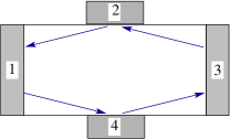
Figure 13: Edge states in a four-terminal measurement. Leads 1 and 3 are the current source and drain, while leads 2 and 4 are the voltage leads.

However, it is essential to emphasize that neither two, nor four-terminal samples (with terminals at well defined voltages) can simultaneously measure both a Hall and a longitudinal resistance. This is obvious for a two-terminal measurement, which can measure a single two-terminal conductance $R_{12,12}$. For a four-terminal geometry (see Fig. 13), consider the case of $n$ filled Landau levels, $\nu=n$. We know that each LL will transport charge through a set of edge states, such as those sketched in Fig. 13. The conductance matrix in this case is:

$$\hat{g}_{4}=n\frac{e^{2}}{h}\left(\begin{array}[c]{cccc}-1&1&0&0\\ 0&-1&1&0\\ 0&0&-1&1\\ 1&0&0&-1\\ \end{array}\right)$$

Taking leads 1 and 3 as the current source and drain, $\hat{I}=(-I,0,I,0)$ and assuming that lead 3 is grounded, one can solve $\hat{I}=\hat{g}_{4}\cdot\hat{V}$ for the other 3 voltages. One finds trivially that $V_{1}=V_{4}=Ih/(ne^{2})$ and $V_{2}=V_{3}=0$. Thus, even though at first sight one might assume that one can measure a Hall resistance $R^{H}=(V_{4}-V_{2})/I$ and a longitudinal resistance $R^{L}=(V_{1}-V_{3})/I$, it turns out that in fact both measurements give resistances exhibiting plateaus at quantized values $h/(ne^{2})$. In other words, both results are related to a Hall resistance (a longitudinal resistance should be zero when $\nu=n$. Note that at transitions between the plateaus, the two resistances need not be equal, since the partially filled LL will introduce other off-diagonal matrix elements. Using the type of analysis we introduced in Section V, one could now easily study what types of correlations might be possible in such a geometry). If one now compares this to a 6-terminal case, it becomes obvious that the four-terminal resistances have no reason to be related to the $R^{H}$ measured in the six-terminals by experimentalists. Thus, in order to simulate and understand the experimental results, it is essential to use the six-terminal geometry.

These considerations show that for mesoscopic samples, a full specification of the experimental setup is absolutely necessary for any interpretation of the measured quantities. For example, the various correlations and symmetries that we studied in this paper only appear in the six-lead setup. Other geometries can be analyzed similarly. A significant result of our work is the proof that an understanding of various possible (robust) correlations can be obtained based on simple arguments regarding the general allowed structure of the conductance matrix, without need for detailed numerical simulations.

Furthermore, we have shown that the full DC response function (the conductance matrix) of a mesoscopic sample is characterized by a large number of parameters (12, for our six-terminal geometry, when we ignore the small tunneling between the left and right-side of the Hall bar). This is to be contrasted with macroscopic samples which only require two parameters, the Hall and longitudinal conductivities $\sigma_{xy}$ and $\sigma_{xx}$, to fully characterize their DC response. A mesoscopic sample obviously has more degrees of freedom to display fluctuations of its resistances.

Appendix A Choosing the right confining potential

The confining potential is needed to define the Hall bar out of the larger area spanned by each LL Hilbert subspace. It is convenient to make a symmetric choice. We take the confining potential to be negative in the region $[-L_{x}/2,L_{x}/2)\times(-L_{y}/2,0)$ (which is thus the Hall bar) and positive in the remaining region $[-L_{x}/2,L_{x}/2)\times(0,L_{y}/2)$ (the inverted Hall bar) and such that $V_{c}(x,y)=-V_{c}(x,y+L_{y}/2)$. On the $y$-edges of the Hall bar we then have $V_{c}(x,-L_{y}/2)=V_{c}(x,0)=0$. Inside most of the Hall bar, the confining potential is equal to $-V_{\rm gap}$, where $V_{\rm gap}>0$ is large enough to confine the electrons to the Hall bar when disorder is added, for all $E_{F}<0$.

The question is how should $V_{c}(x,y)$ behave near the Hall bar edges, at $x=\pm L_{x}/2$ or $y=-L_{y}/2,0$. For instance, $V_{c}$ could vary smoothly or abruptly from $-V_{gap}$ to 0, as the $y$-edges are approached. On the $x$-edges, we could take $V_{c}=0$ or $-V_{gap}$. Two of the possible choices are shown in Fig. 14. The shape of $V_{c}$ near the edges is critical for the quality of the simulation, as we show here.

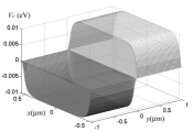
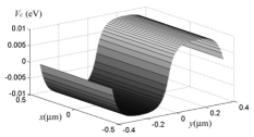
Figure 14: Two of the tested confining potentials. Left: This potential has discontinuous changes at $y=0$ and $y=\pm L_{y}/2$, and is smoothly connected to zero on the $x$-edges. Right: An improved potential with open ends and smooth $y$-edges.

Since little is known about the real shape of the confining potential, we test the various choices by analyzing the IQHE transition from $R^{H}=h/e^{2}$ to $R^{H}=h/(2e^{2})$, in the absence of disorder. The computation is done as described in the text, but with $V_{d}=0$. We add a $\hat{g}^{(0)}$ to the calculated $\hat{g}(\nu)$, to account for the contribution of an underlying, filled LL. These simulations were carried on smaller samples, to save CPU time. The results should show: (1) a sharp transition of $R^{H}$ from ${h/e^{2}}$ to $h/(2e^{2})$; (2) the built-in particle-hole symmetry of the Hamiltonian, i.e. symmetry of the results about $E_{F}=0$ (this is a consequence of choosing a symmetric confining potential and symmetric contact states for the terminals); (3) the two Hall resistances are always equal, and so are the two longitudinal resistances (in the absence of disorder, the potential has rectangular symmetry.)

Figure 14 shows two confining potentials which were used for testing purposes. Typical results of tests using the potential in the right panel of Fig. 14 are shown in Fig. 15 and 16. We found several features of the confining potential that result in unrealistic, unphysical results. First, abrupt changes of the confining potential near the $y$-edges, such as shown in the left panel of Fig. 14, result in strong, fast oscillations in the resistances (similar to those displayed in Fig. 15(b), but with an amplitude of order $h/e^{2}$). Secondly, raising the confining potential to near zero at the $x$-edges, as shown in the same case, also leads to undesired consequences, for example half quantization $R^{H}=R^{L}=h/(2e^{2})$ over a considerable energy range. This is because leads 1 and 4 are only connected to the left-most and right-most LL states. In this case, the energies of these states are close to zero, so they appear to be huge barriers blocking the electrons on the lead to enter the sample. Electrons can only tunnel through these barriers with very small probabilities, and no chiral currents can exit at the $x$-edges unless $E_{F}\approx 0$. In other words, this is equivalent to having very bad contacts, a situation which is avoided in the experiments.

The right panel of Fig. 14 shows an improved confining potential. The confining potential varies smoothy near the $y$-edges, and the $x$-edges are no longer fixed at constant value. The $y$-edges are smooth because in a real sample, we do expect a smooth rise of the confining potential on the edges of the Hall bar. Its gradient is determined by how the 2DES is defined on the sample, as well as various screening effects.

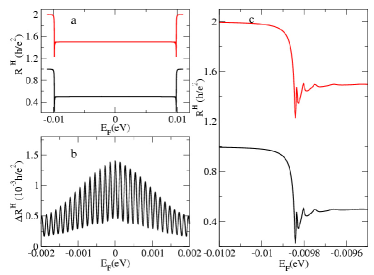
Figure 15: Hall resistances calculated for the confining potential shown in Fig. 14 (right), $R^{H}_{14,62}$ (grey) and $R^{H}_{14,53}$ (black). (a) The overview of the entire energy interval scanned by Fermi energy $E_{F}$. Here, $R^{H}_{14,53}$ has been shifted up by one unit. (b) Amplified view of the very small oscillations close to $E_{F}=0$, $\Delta R^{H}=R^{H}-{h\over 2e^{2}}$. (c) Amplified view of the transition from $R^{H}={h\over e^{2}}$ to $R^{H}={h\over 2e^{2}}$.

Figure 15 plots the Hall resistances calculated with $V_{c}$ shown in Fig. 14 (right). Panel (a) shows an overview of the data. Here $V_{\rm gap}=10$meV, so that $E_{F}$ was varied over a range spanning the entire confining potential. Particle-hole symmetry is obvious. Panel (b) zooms in on the central region close to $E_{F}=0$ in panel (a) and reveals the minute scale of oscillations in $R^{H}$. In this regime, the edge states have been fully established, and the total conductance matrix is almost exactly $2\hat{g}^{(0)}$. The small oscillations also exhibit the built-in particle-hole symmetry. Panel (c) zooms in on the transition region. One can see that the transition from first to the second plateau occurs within a small energy interval. This is because in the absence of disorder, the edge states are established immediately once $E_{F}>-V_{\rm gap}$. In all panels, we see that the two Hall resistances are indeed identical.

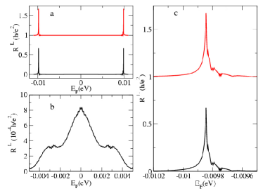
Figure 16: Longitudinal resistances calculated for the confining potential shown in Fig. 14(right), $R^{H}_{14,62}$ (grey) and $R^{H}_{14,53}$ (black). (a) The overview of the entire energy interval scanned by Fermi energy $E_{F}$. Here, $R^{H}_{14,53}$ has been shifted up by one unit. (b) Amplified view of the very small variations close to $E_{F}=0$. (c) Amplified view of the IQHE transition.

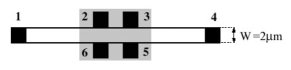
Figure 17: A sketch of the sample used by Peled et al.,(Peled et al., 2003a, b; Peled04, ) drawn to scale. The region spanned by our LL Hilbert subspace is comparable to the size of the shaded area.

Figure 16 shows the longitudinal resistances for the same simulation. All the expected symmetries are again observed. Except for the very narrow interval of energies where the transition takes place, the longitudinal resistances are vanishingly small. This is expected, since for all energies except near $\pm V_{\rm gap}$ all transport is due to edge modes, which do not contribute to $R^{L}$. The small deviations from zero near $E_{F}=0$ are magnified in panel (b). In panel (c), we show the peaks associated with the transition. The symmetries observed in the results confirm the numerical accuracy of the simulations. We are now confident that in the absence of disorder, the simulation shows a clear integer quantum Hall transition. Thus, we have confidence in attributing extra features in the full simulations to the effects of the disorder.

As we just showed, the confining potential of Fig. 14 (right) gives physically reasonable results. However, we make one more modification, to account for the short size of the samples we use in numerical simulations. Fig. 17 shows the geometry of the real sample used in the experiments.Peled et al. (2003a, b); Peled04 The length of the real sample is approximately 20 $\mu$m. Given our computational resources, we simulate the relatively short shaded area, so that after adding the confining potential, our Hall bar has the same thickeness and distance between the 4 central voltage terminals, but is only 4 $\mu$m long. Thus, our current source and drain (leads 1 and 4) are much closer to the voltage probes than in experiments.

Because of this short distance, we frequently observe direct tunneling between leads 1 or 4 and their nearest neighbor terminals (2, 6 respectively 3, 5). In the simulation, this kind of tunneling leads to large symmetric matrix elements in the conductance matrix, e.g. $g_{12}\approx g_{21}\sim e^{2}/h$, and abnormal behavior of $R^{L}$ and $R^{H}$. Experimentalists take great care to avoid direct tunneling between leads, which constitutes a short-circuit. To avoid such direct tunneling in the simulation, we add triangular potential barriers in the corners of the Hall bar. With these, the edges are effectively prolonged, corresponding to an increased separation between the voltage probes and current source and drain. Fig. 2 shows the final form of the confining potential used in our simulations with six terminals.

References

- von Klitzing et al. (1980) K. v. Klitzing, G. Dorda, and M. Pepper, Phys. Rev. Lett. 45, 494 (1980).
- Středa (1982) P. Středa, J. Phys. C: Solid State Phys. 15, L717 (1982).
- Thouless et al. (1982) D. J. Thouless, M. Kohmoto, M. P. Nightingale, and M. den Nijs, Phys. Rev. Lett. 49, 405 (1982).
- Rammal et al. (1983) R. Rammal, G. Toulouse, M. T. Jaekel, and B. I. Halperin, Phys. Rev. B 27, R5142 (1983).
- Büttiker (1988) M. Büttiker, Phys. Rev. B 38, 9375 (1988).
- Pruisken (1987) A. M. M. Pruisken, Nucl. Phys. B285, 719 (1987).
- Wei et al. (1988) H. P. Wei, D. C. Tsui, M. A. Paalanen, and A. M. M. Pruisken, Phys. Rev. Lett. 61, 1294 (1988).
- Huckestein and Kramer (1990) B. Huckestein and B. Kramer, Phys. Rev. Lett. 64, 1437 (1990).
- Huo and Bhatt (1992) Y. Huo and R. N. Bhatt, Phys. Rev. Lett. 68, 1375 (1992).
- Huckestein (1995) B. Huckestein, Rev. Mod. Phys. 67, 357 (1995).
- Beenakker (1997) C. W. J. Beenakker, Rev. Mod. Phys. 69, 731 (1997).
- (12) Mesoscopic Phenomena in Solids, edited by B. L. Altshuler, P. A. Lee, and R. A. Webb (North-Holland, New York, 1991).
- (13) P. A. Lee, A. D. Stone and H. Fukuyama, Phys. Rev. B 35, 1039 (1987), and references therein.
- Peled et al. (2003a) E. Peled, D. Shahar, Y. Chen, D. L. Sivco, and A. Y. Cho, Phys. Rev. Lett. 90, 246802 (2003a).
- Peled et al. (2003b) E. Peled, D. Shahar, Y. Chen, E. Diez, D. L. Sivco, and A. Y. Cho, Phys. Rev. Lett. 91, 236802 (2003b).
- (16) E. Peled, Y. Chen, E. Diez, D. C. Tsui, D. Shahar, D. L. Sivco, and A. Y. Cho, Phys. Rev. B 69, 241305(R) (2004).
- (17) C. Zhou and M. Berciu, Europhys. Lett. 69, 602 (2005).
- Baranger and Stone (1989) H. U. Baranger and A. D. Stone, Phys. Rev. B 40, 8169 (1989).
- (19) C. Zhou and M. Berciu, Phys. Rev. B 70, 165318 (2004).
- Shahar et al. (1997) D. Shahar, D. C. Tsui, M. Shayegan, E. Shimshoni, and S. L. Sondhi, Phys. Rev. Lett. 79, 479 (1997).
- (21) Spin-dependent scattering –although it may be very weak – is necessary for the relaxation of electrons to the lowest spin-polarized LL as the magnetic field is increased.
- Jain and Kivelson (1988) J. K. Jain and S. A. Kivelson, Phys. Rev. Lett. 60, 1542 (1988).
- (23) S. Cho and M. P. A. Fisher, Phys. Rev. B 55, 1637 (1997).
- (24) Ziqiang Wang, Bozidar Jovanovic, and Dung-Hai Lee, Phys. Rev. Lett. 77, 4426 (1996).
- (25) J. T. Chalker and P. D. Coddington, J. Phys. C 21, 2665 (1988).
- (26) T. Ando, Phys. Rev. B 49, 4679 (1994).
- (27) T. Ando, Phys. Rev. B 44, 8017 (1991).
- (28) S. Datta, Electronic Transport in Mesoscopic Systems (Cambridge University Press, Cambridge, 1997).
- (29) P. Streda, J. Kucera and A. H. MacDonald, Phys. Rev. Lett. 59, 1973 (1987).
- Büttiker (1986) M. Büttiker, Phys. Rev. Lett. 57, 1761 (1986).