Interference Effects on Kondo-Assisted Transport
through Double Quantum Dots

Abstract

We systematically investigate electron transport through double quantum dots with particular emphasis on interference induced via multiple paths of electron propagation. By means of the slave-boson mean-field approximation, we calculate the conductance, the local density of states, the transmission probability in the Kondo regime at zero temperature. It is clarified how the Kondo-assisted transport changes its properties when the system is continuously changed among the serial, parallel and T-shaped double dots. The obtained results for the conductance are explained in terms of the Kondo resonances influenced by interference effects. We also discuss the impacts due to the spin-polarization of ferromagnetic leads.

I Introduction

Recent intensive investigations of electron transport through quantum dot (QD) systems have uncovered novel correlation effects in nanoscale systems. In particular, the observation Gold ; Cronen of the Kondo effect in QD systems Glaz ; Ng ; MW ; Kawa ; Ogu opened a new path for the investigation of strongly correlated electrons, which has stimulated further experimental and theoretical studies in this field Kouwen . More recently, a variety of QD systems, such as an Aharonov-Bohm ring with QD, double quantum dot (DQD) systems, etc, have been fabricated. An interesting new feature in these systems is the interference effects induced via multiple paths of electron propagation Hack . For example, such interference effects have been clearly observed in the Aharonov-Bohm ring with QD Yaco ; Buks ; WG ; Ji ; Koba .

When electron correlations due to the Kondo effect are affected by such interference, transport properties exhibit remarkable properties. There have been a number of theoretical works on DQD systems in this context. For example, it was pointed out that the DQD system shows the dramatic suppression of the Kondo-assisted transport due to the interference when the DQD is arranged in the parallel geometry Shimizu ; Rosa ; Boese ; Imamura ; Chen ; LuYu ; Lei ; tanaka2 , whereas such interference effects do not appear in the serial DQD Lang ; George ; Rosa ; Eto ; Eto2 ; Busser1 ; Izumi ; sakano ; Jeong . More recently, slightly different DQD systems with the parallel geometry, where the two dots are connected via the exchange coupling LuYu or the tunneling Lei ; tanaka2 , have been studied. It has been pointed out that the Kondo-assisted transport in these cases exhibits different properties from the above simple DQD case without the inter-dot coupling. The T-shaped DQD Tae ; Kikoin ; Taka ; Busser2 ; Apel ; Corna is another prototype of such correlated systems, for which the special arrangement of the DQD provides an additional path of electron propagation, giving rise to the interference effects. This system also shows somewhat different transport properties from the parallel DQD case, but the detailed analysis has not been done systematically. In any case, the interplay of the Kondo effect and the interference provides intriguing phenomena due to electron correlations in the DQD systems. It is thus interesting to systematically study how the interference together with the Kondo effect affects characteristic transport properties in a variety of DQD systems.

Motivated by the above hot topics, we investigate Kondo-assisted transport properties in DQD systems, when the geometry of the system is systematically changed among the serial, parallel and T-shaped DQD. We pay our particular attention to the Kondo effect under the influence of the interference due to different paths. We also discuss the DQD systems with ferromagnetic (FM) leads. This is stimulated by the recent extensive study of spin-dependent transport through a QD coupled to FM leads in the context of spintronics Wang ; Zhang ; Sergu ; Lopez ; Koing ; Utumi ; Marti ; JiMa ; BinDon ; Choi ; tanaka1 ; Ralph . Since the Kondo effect is sensitive to the internal spin degrees of freedom, notable phenomena caused by the FM leads are expected to appear in transport properties.

This paper is organized as follows. In the next section, we introduce the model and briefly summarize the formulation based on the Keldysh Green function method. Then in Sec. III, we calculate the local density of states (DOS) and the linear conductance at zero temperature by the slave-boson mean field approximation AC ; Cole for the serial, parallel and T-shaped DQD systems. We discuss characteristic transport properties induced by the Kondo effect under the influence of interference. The effect of the spin-polarization due to the FM leads is also addressed. A brief summary is given in the last section.

II Model and Method

Figure 1: DQD system connected by the inter-dot tunneling $t_{c}$: $\Gamma^{\alpha}_{m,m\sigma}(\alpha=L,R$ and $m=1,2)$ represents the resonance width due to transfer between the $m$-th dot and the $\alpha$-th lead for an electron with spin $\sigma$. By changing the ratio of tunneling amplitudes, we continuously change the system among the serial, parallel and T-shaped DQD.

We consider a DQD system shown schematically in Fig. 1 Shimizu ; Rosa ; Boese ; Imamura ; Chen ; LuYu ; Lei ; tanaka2 ; Gueva . In the following discussions, the intra-dot Coulomb interaction is assumed to be sufficiently large, so that double occupancy on each QD is forbidden. This assumption allows us to use a slave-boson representation AC ; Cole of correlated electrons in the dots. In this representation, the creation (annihilation) operator of electrons in the dot $m$ ($m=1,2$), $d_{m\sigma}^{\dagger}$($d_{m\sigma}$), is replaced by $d_{m\sigma}^{\dagger}\to f_{m\sigma}^{\dagger}b_{m}$ ($d_{m\sigma}\to b_{m}^{\dagger}f_{m\sigma}$), where $b_{m}$ ($f_{m\sigma}$) is the slave-boson (pseudo-fermion) annihilation operator for an empty state (singly occupied state). We can thus model the system in Fig. 1 with a $N$(=2) fold degenerate Anderson Hamiltonian,

$$H = \sum_{k_{\alpha},\sigma}\varepsilon_{k_{\alpha}\sigma}c_{k_{\alpha}\sigma}^{\dagger}c_{k_{\alpha}\sigma}+\sum_{m,\sigma}\varepsilon_{m\sigma}f_{m\sigma}^{\dagger}f_{m\sigma}$$ (1)

$$+ \frac{t_{c}}{N}\sum_{\sigma}(f_{1\sigma}^{\dagger}b_{1}b_{2}^{\dagger}f_{2\sigma}+h.c)$$

$$+ \frac{1}{\sqrt{N}}\sum_{k_{\alpha},m,\sigma}(V_{\alpha m\sigma}c_{k_{\alpha}\sigma}^{\dagger}b_{m}^{\dagger}f_{m\sigma}+h.c.)$$

$$+ \sum_{m}\lambda_{m}(\sum_{\sigma}f_{m\sigma}^{\dagger}f_{m\sigma}+b_{m}^{\dagger}b_{m}-1).$$

The first and second terms in the Hamiltonian (1) represent the electronic states in the leads and the dots, where $c_{k_{\alpha}\sigma}^{\dagger}$($c_{k_{\alpha}\sigma}$) is the creation (annihilation) operator of an electron with energy $\varepsilon_{k_{\alpha}\sigma}$ and spin $\sigma$ in the lead $\alpha$ ($\alpha=L,R$). The coupling between the two dots (between the lead and the dot) is given by the third (fourth) term in the Hamiltonian (1). The last term with the Lagrange multiplier $\lambda_{m}$ is introduced so as to incorporate the constraint imposed on the slave particles, $\sum_{\sigma=\uparrow,\downarrow}{f_{m\sigma}^{\dagger}f_{m\sigma}}+b_{m}^{\dagger}b_{m}=1$. The mixing term $V_{\alpha m\sigma}$ in the Hamiltonian (1) leads to the linewidth function

$$\Gamma_{m,n\sigma}^{\alpha}(\varepsilon)=\pi\sum_{k_{\alpha}}V_{\alpha m\sigma}V^{*}_{\alpha n\sigma}\delta(\varepsilon-\varepsilon_{k_{\alpha}\sigma}).$$ (2)

In the wide band limit, $\Gamma_{m,n\sigma}^{\alpha}(\varepsilon)$ is reduced to an energy-independent constant $\Gamma_{m,n\sigma}^{\alpha}$.

According to Ref. Gueva , we interpolate the serial DQD and parallel DQD by continuously changing $x=\Gamma_{1,1\sigma}^{R}=\Gamma_{2,2\sigma}^{L}$ with the resonance width $\Gamma_{1,1\sigma}^{L}(=\Gamma_{2,2\sigma}^{R})$ fixed as unity. Note that at $x=0$ the model is reduced to the DQD connected in series (serial DQD, Fig. 2(a)), and at $x=1$ the parallel DQD. Similarly, we modify the tunneling amplitudes in a different way, i.e. we change $y=\Gamma_{2,2\sigma}^{R}=\Gamma_{2,2\sigma}^{L}$ by keeping the resonance width $\Gamma_{1,1\sigma}^{L}(=\Gamma_{1,1\sigma}^{R})$ fixed as unity. Then we can naturally interpolate the parallel DQD ($y=1$) and the T-shaped DQD ($y=0$), where only one of the two dots is connected to the leads, as shown in Fig. 2(b).

Figure 2: (a) Serial DQD system, which is a special case of Fig. 1 ($\Gamma_{1,1\sigma}^{R}=\Gamma_{2,2\sigma}^{L}=0$). (b) T-shaped DQD system realized at $\Gamma_{2,2\sigma}^{L}=\Gamma_{2,2\sigma}^{R}=0$ in Fig. 1.

To analyze the model, we apply the mean-field approximation to the slave-boson treatment AC ; Cole , in which boson fields are approximated by their static mean values, $b_{m}(t)/\sqrt{N}\to\langle b_{m}(t)\rangle/\sqrt{N}=\tilde{b}_{m}$. We introduce the renormalized quantities $\tilde{V}_{\alpha m\sigma}=V_{\alpha m\sigma}\tilde{b}_{m}$, $\tilde{t}_{c}=t_{c}\tilde{b}_{1}\tilde{b}_{2}$, and $\tilde{\varepsilon}_{m\sigma}=\varepsilon_{m\sigma}+\lambda_{m}$. The mean-field values of $\tilde{b}_{1},\tilde{b}_{2},\lambda_{1}$ and $\lambda_{2}$, are determined by the following set of self-consistent equations, which are derived by the equation of motion method for the non-equilibrium Keldysh Green functions Rosa ; Lang ,

$$\tilde{b}_{1(2)}^{\,2}-i\sum_{\sigma}\int\frac{d\varepsilon}{4\pi}G_{1,1(2,2)\sigma}^{<}(\varepsilon)=\frac{1}{2},$$ (3)

$$(\tilde{\varepsilon}_{1(2)\sigma}-\varepsilon_{1(2)\sigma})\,\tilde{b}_{1(2)}^{\,2}$$

$$\quad\quad-i\sum_{\sigma}\int\frac{d\varepsilon}{4\pi}(\varepsilon-\tilde{\varepsilon}_{1(2)\sigma})\,G_{1,1(2,2)\sigma}^{<}(\varepsilon)=0.$$ (4)

In the above equations, $G_{1,1(2,2)\sigma}^{<}(\varepsilon)$ is the Fourier transform of the Keldysh Green function $G_{1,1(2,2)\sigma}^{<}(t-t^{\prime})\equiv i\langle f_{1(2)\sigma}^{\dagger}(t)f_{1(2)\sigma}(t^{\prime})\rangle$. Eq. (3) represents the constraint imposed on the slave particles, while Eq. (4) is obtained from the stationary condition that the boson field is time-independent at the mean-field level. From the equation of motion of the operator$f_{m\sigma}$ MW ; Lang ; Keldysh , we have the explicit form of the Green function,

$$G_{1,1(2,2)\sigma}^{<}(\varepsilon)=\frac{2i}{|D_{\sigma}(\varepsilon)|^{2}} \Big{\{} \left(f_{L}(\varepsilon)\tilde{\Gamma}_{1,1(2,2)\sigma}^{L}+f_{R}(\varepsilon)\tilde{\Gamma}_{1,1(2,2)\sigma}^{R}\right)\left(\varepsilon-\tilde{\varepsilon}_{2(1)\sigma}+i\tilde{\Gamma}_{2,2(1,1)\sigma}\right)\left(\varepsilon-\tilde{\varepsilon}_{2(1)\sigma}-i\tilde{\Gamma}_{2,2(1,1)\sigma}\right)$$ (5)

$$+ \left(f_{L}(\varepsilon)\tilde{\Gamma}_{1,2(2,1)\sigma}^{L}+f_{R}(\varepsilon)\tilde{\Gamma}_{1,2(2,1)\sigma}^{R}\right)\left(\varepsilon-\tilde{\varepsilon}_{2(1)\sigma}+i\tilde{\Gamma}_{2,2(1,1)\sigma}\right)\left(\tilde{t}_{c}+i\tilde{\Gamma}_{2,1(1,2)\sigma}\right)$$

$$+ \left(f_{L}(\varepsilon)\tilde{\Gamma}_{2,1(1,2)\sigma}^{L}+f_{R}(\varepsilon)\tilde{\Gamma}_{2,1(1,2)\sigma}^{R}\right)\left(\tilde{t}_{c}-i\tilde{\Gamma}_{1,2(2,1)\sigma}\right)\left(\varepsilon-\tilde{\varepsilon}_{2(1)\sigma}-i\tilde{\Gamma}_{2,2(1,1)\sigma}\right)$$

$$+ \left(f_{L}(\varepsilon)\tilde{\Gamma}_{2,2(1,1)\sigma}^{L}+f_{R}(\varepsilon)\tilde{\Gamma}_{2,2(1,1)\sigma}^{R}\right)\left(\tilde{t}_{c}-i\tilde{\Gamma}_{1,2(2,1)\sigma}\right)\left(\tilde{t}_{c}+i\tilde{\Gamma}_{2,1(1,2)\sigma}\right)\Big{\}},$$

with $\tilde{\Gamma}_{m,n\sigma}^{\alpha}=\tilde{b}_{m}\tilde{b}_{n}\Gamma_{m,n\sigma}^{\alpha}$ and $\tilde{\Gamma}_{m,n\sigma}=\tilde{\Gamma}_{m,n\sigma}^{L}+\tilde{\Gamma}_{m,n\sigma}^{R}\,(m,n=1,2$ and $\alpha=L,R)$, where the denominator of Eq. (5) is

$$D_{\sigma}(\varepsilon) = (\varepsilon-\tilde{\varepsilon}_{1\sigma}+i\tilde{\Gamma}_{1,1\sigma})(\varepsilon-\tilde{\varepsilon}_{2\sigma}+i\tilde{\Gamma}_{2,2\sigma})$$ (6)

$$-(\tilde{t_{c}}-i\tilde{\Gamma}_{1,2\sigma})(\tilde{t_{c}}-i\tilde{\Gamma}_{2,1\sigma}).$$

From the renormalized parameters determined self-consistently in Eqs. (3) and (4), we obtain the DOS for the dot-1 and dot-2 as

$$\rho_{1(2),\sigma}(\varepsilon)=-\frac{\tilde{b}_{1(2)}^{\,2}}{\pi}\textrm{Im}\left[\frac{\varepsilon-\tilde{\varepsilon}_{2(1)\sigma}+i\tilde{\Gamma}_{2,2(1,1)\sigma}}{D_{\sigma}(\varepsilon)}\right]_{.}$$ (7)

By applying the Landauer formula in steady state, we can derive the current $I$ through the two dots MW ; Lang ; Keldysh ,

$$I=\frac{2e}{h}\sum_{\sigma}\int d\varepsilon(f_{L}(\varepsilon)-f_{R}(\varepsilon))T_{\sigma}(\varepsilon),$$ (8)

where the transmission probability is given by

$$T_{\sigma}(\varepsilon) = \frac{2}{D_{\sigma}(\varepsilon)}\left[\tilde{t}_{c}\left(\sqrt{\tilde{\Gamma}_{1,1\sigma}^{L}\tilde{\Gamma}_{2,2\sigma}^{R}}+\sqrt{\tilde{\Gamma}_{2,2\sigma}^{L}\tilde{\Gamma}_{1,1\sigma}^{R}}\right)\right.$$

$$\!\!\!\!\!\!\left.+\sqrt{\tilde{\Gamma}_{1,1\sigma}^{L}\tilde{\Gamma}_{1,1\sigma}^{R}}(\varepsilon-\tilde{\varepsilon}_{2\sigma})+\sqrt{\tilde{\Gamma}_{2,2\sigma}^{L}\tilde{\Gamma}_{2,2\sigma}^{R}}(\varepsilon-\tilde{\varepsilon}_{1\sigma})\right]_{.}^{2}$$

We can thus compute the linear conductance $G_{V=0}=dI/dV|_{V=0}$ by

$$G_{V=0}=\frac{2e^{2}}{h}\sum_{\sigma}T_{\sigma}(\varepsilon=0).$$ (10)

III Numerical Results

In this section, we discuss transport properties at zero temperature for the DQD systems with the serial, parallel and T-shaped geometries. We also show the results obtained for the DQD systems connected to spin-polarized leads.

III.1 From serial to parallel DQD

Let us first discuss how the interference affects Kondo-assisted transport when we continuously change the system from the serial ($x=0$) to parallel ($x=1$) DQD. For simplicity, we deal with the symmetric dots in the Kondo regime with $\varepsilon_{1}=\varepsilon_{2}=-3\Gamma_{0}$. The band width of the leads is taken as $D=60\Gamma_{0}$, where $\Gamma_{0}=\Gamma_{1,1}^{L}=\Gamma_{2,2}^{R}$ (unit of energy), and the Fermi level of the leads is chosen as the origin of energy.

III.1.1 non-polarized leads

We begin with the DQD system coupled to non-polarized leads: a brief report on this part can be found in Ref. tanaka2 . We should also mention two closely related works presented recently by Zhang et al. LuYu and Dong et al. Lei , who treated transport properties of similar models with non-polarized leads. Here, we briefly summarize our results, which will make clear how distinctly the interference appears in the parallel DQD with and without the spin polarization.

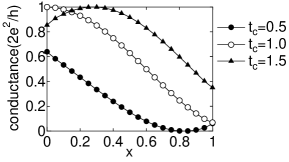
Figure 3: Linear conductance as a function of $x=\Gamma_{1,1\sigma}^{R}=\Gamma_{2,2\sigma}^{L}$, where we set $\Gamma_{2,2\sigma}^{R}=\Gamma_{1,1\sigma}^{L}=1$.

Figure 3 shows the linear conductance $G_{V=0}$ as a function of $x$ for several values of the inter-dot coupling $t_{c}$. Starting from the serial DQD ($x=0$), we see that the conductance has a maximum around $x=0.3$ for $t_{c}=1.5$, whereas it monotonically decreases for $t_{c}=1$ or takes a tiny minimum structure around $x=0.8$ for $t_{c}=0.5$. In any case, as the system approaches the parallel DQD ($x\sim 1$), the conductance is considerably suppressed. These characteristic properties come from the Kondo effect modified by the interference, which is clearly seen in the local DOS and the transmission probability shown below.

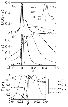
Figure 4: (a)DOS for $t_{c}=1.5$: $x=0.2,0.5$ and $0.8$. Inset shows the DOS at $x=0$. (b)The transmission probability $T(\varepsilon)$ for $t_{c}=1.5$. (c)Enlarged picture of (b) around $\varepsilon=0$.

The local DOS of the dots around the Fermi energy $\varepsilon=0$ is shown in Fig. 4(a) for a typical value of $t_{c}=1.5$. For the serial case ($x=0$), the Kondo resonance has a small splitting caused by the inter-dot coupling $t_{c}$ Lang ; George ; Rosa ; Eto ; Eto2 ; Busser1 ; Izumi . The Kondo temperature in this case is roughly estimated as 0.02$\Gamma_{0}$, as seen in the inset of Fig. 4(a). As $x$ increases, one of the resonances (lower-energy side), which is composed of the ”bonding” Kondo state of the DQD, becomes sharp around the Fermi energy, while the other ”anti-bonding” Kondo state (higher-energy side) is broadened above the Fermi level Shimizu ; LuYu ; Lei ; tanaka2 ; Busser2 ; Gueva . This tendency results from the fact that the bonding state is almost decoupled from the leads while the anti-bonding state is still tightly connected to the leads as $x\rightarrow 1$. As a result, the renormalization of each Kondo temperature occurs: for instance, the Kondo temperature for the narrower (wider) resonance is about $0.01\Gamma_{0}$ (0.2$\Gamma_{0}$) at $x=0.5$.

Such two modified Kondo resonances also appear in the transmission probability $T(\varepsilon)$ (Fig. 4(b)). A remarkable point is that the sharp resonance in $T(\varepsilon)$ around the Fermi energy in Fig. 4(b) becomes asymmetric and acquires a dip structure (more clearly seen in Fig. 4(c)). The asymmetric peak, which may be regarded as a Fano-like structure, is caused by the interference between two conduction channels having two distinct Kondo resonances. This type of interference plays a crucial role to determine the Kondo-assisted conductance in DQD systems Shimizu ; LuYu ; Lei ; tanaka2 ; Busser2 ; Gueva . With the increase of $x$, the maximum of the asymmetric resonance of $T(\varepsilon)$ in Fig. 4(c) passes through the Fermi energy, from which we see why the linear conductance $G_{V=0}$ for $t_{c}=1.5$ in Fig. 3 has a maximum around $x=0.3$ and then decreases. When we choose different values of $t_{c}$(=1.0, 0.5), analogous interference effects occur, reducing the conductance substantially when the system approaches the parallel DQD. Therefore, we see that apart from the detailed dependence, the characteristic behavior of the conductance in Fig. 3 is due to the Kondo-assisted transport modified by the interference effects.

Here we make a brief comment on the related work by Zhang et al. LuYu , who treated an analogous DQD system (two dots are connected via the exchange coupling $J$). We have confirmed that for a given choice of the inter-dot coupling $t_{c}$ in the present model and $J$ in their model, the conductance exhibits similar interference effects. However, there are several different properties between these two models. For example, in the serial-DQD limit ($x=0$), the former (latter) model has a finite (vanishing) conductance. Also, the gate-voltage control of the dot levels shows an opposite tendency: the increase of the dot-level enhances (suppresses) the effect of the inter-dot coupling $t_{c}$ ($J$). These different properties come from the fact that the former model allows charge fluctuations between the dots while the latter model prohibits them. We will come back to this point later again in the discussions of the T-shaped DQD.

III.1.2 spin-polarized leads

We next discuss the influence of the spin-polarized leads on the conductance, where the leads $L$ and $R$ have the same orientation of spin-polarization. The spin-polarization of the leads gives rise to the difference in the DOS between up- and down-spin conduction electrons, so that the resonance width $\Gamma_{m,n\sigma}^{\alpha}$ should be spin-dependent. To represent how large the strength of the spin polarization is, we introduce the effective spin-polarization strength p, following the definition given in the literature Wang ; Zhang ; Sergu ; Lopez ; Koing ; Utumi ; Marti ; JiMa ; BinDon ; Choi ; tanaka1 ; Julli ; Slon :

$$p=\frac{\Gamma_{m,m\sigma}^{\alpha}-\Gamma_{m,m\bar{\sigma}}^{\alpha}}{\Gamma_{m,m\sigma}^{\alpha}+\Gamma_{m,m\bar{\sigma}}^{\alpha}}\,\,\,(0\leq p\leq 1)\,.$$ (11)

This definition of p is equivalent to the condition imposed on $\Gamma_{m,m\sigma}^{\alpha}$,

$$\Gamma_{m,m\uparrow}^{L(R)} = (1+p)\Gamma_{m,m}^{L(R)}|_{p=0},$$

$$\Gamma_{m,m\downarrow}^{L(R)} = (1-p)\Gamma_{m,m}^{L(R)}|_{p=0},$$ (12)

for up-spin (majority-spin) electrons and down-spin (minority-spin) electrons, respectively. We think that the above simple assumption captures some essential effects due to the polarization of the leads.

Since the system for small $x$ shows the $p$-dependence similar to the serial case ($x=0$) studied elsewhere tanaka1 , we discuss spin-polarized transport at $x=0.8$, which includes essential properties inherent in the parallel setup ($x\sim 1$).

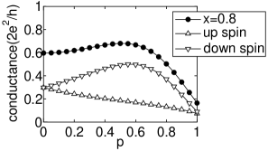
Figure 5: Linear conductance as a function of the spin-polarization strength $p$ for $t_{c}=1.5$ and $x=0.8$. The contribution from up- and down-spin electrons is also shown.

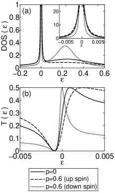
Figure 6: (a) DOS of up- and down-spin electrons connected to normal leads ($p=0$) and ferromagnetic leads ($p=0.6$). We assume $t_{c}=1.5$ and $x=0.8$. Inset: Enlarged picture around $\varepsilon=0$. (b)Transmission probability $T(\varepsilon)$ of up- and down-spin electrons.

In Fig. 5 the linear conductance is shown as a function of the spin-polarization strength $p$ for the inter-dot coupling $t_{c}=1.5$ at $x=0.8$. As $p$ increases, the contribution of down-spin electrons to the total conductance begins to increase, giving rise to a maximum around $p=0.6$, whereas the contribution of up-spin electrons decreases monotonically. The above behavior due to the spin-polarization is explained in terms of the modified Kondo resonances and the asymmetric structure of $T(\varepsilon)$ around the Fermi energy. Shown in Fig. 6(a) is the DOS of up- and down-spin electrons for $p=0.6$, which is compared with that for $p=0$. The introduction of the spin-polarization of leads broadens the Kondo resonance of up-spin electrons whereas it sharpens that of down-spin electrons. Such change in the widths of the Kondo resonances (inset of Fig. 6(a)) modifies the asymmetric nature of the transmission probability $T(\varepsilon)$, as seen in Fig. 6(b): the asymmetric structure in $T(\varepsilon)$ of up-spin electrons for $p=0.6$ is smeared, while that of down-spin electrons gets sharp. The transmission probability at the Fermi energy for up-spin electrons thus decreases with the increase of $p$, so that the contribution of up-spin electrons to the conductance goes down monotonically. However, the conductance of down-spin electrons takes a maximum when the asymmetric peak of $T(\varepsilon)$ reaches the Fermi energy, as shown in Fig. 5. Similar considerations can be applied to other choices of the parameters $t_{c}=0.5$ and $1.0$. In any case in the Kondo regime, the spin polarization changes the asymmetric structure of $T(\varepsilon)$ more significantly for down-spin (minority-spin) electrons, making their contribution to the conductance more dominant.

III.2 From parallel to T-shaped DQD

We now discuss how the Kondo-assisted transport changes its character when the system is changed continuously from the parallel DQD to the T-shaped DQD. For this purpose, we change the resonance widths $y=\Gamma_{2,2\sigma}^{L}=\Gamma_{2,2\sigma}^{R}$ by keeping $\Gamma_{1,1\sigma}^{L}=\Gamma_{1,1\sigma}^{R}$ fixed as unity. At $y=0$, the dot-2 is decoupled from two leads and is connected only to the dot-1 via tunneling $t_{c}$ (T-shaped geometry shown in Fig. 2(b)). On the other hand, the system with $y\sim 1$ exhibits properties characteristic of the parallel DQD. In the following calculation, we assume $\Gamma_{1,1\sigma}^{L}=\Gamma_{1,1\sigma}^{R}$ and take $\Gamma_{0}=\Gamma_{1,1}^{L}|_{p=0}+\Gamma_{1,1}^{R}|_{p=0}$ as the unit of energy.

III.2.1 non-polarized leads

Figure 7: DOS of (a) dot-1 and (b) dot-2 around the Fermi energy. (c)The corresponding transmission probability $T(\varepsilon)$. We set $t_{c}=2$ and $\varepsilon_{1}=\varepsilon_{2}=-3.0$.

In Figs. 7(a) and (b) the DOS is shown in the Kondo regime with $\varepsilon_{1}=\varepsilon_{2}=-3.0$. For $y=0.8$, the DOS has the Kondo resonance with the double-peak structure both for the dot-1 and the dot-2, where one of the two peaks is sharp around the Fermi energy while the other is broad above the Fermi energy. We have already encountered such situation in the previous subsection for the system close to the parallel dot ($x\sim 1$). However, when the system approaches the T-shaped DQD ($y\rightarrow 0$), quite different behavior emerges. As $y$ decreases, the Kondo resonance of the dot-1 gradually becomes symmetric with a sharp dip structure at $\varepsilon\sim 0$, whereas the DOS of the dot-2 develops a single Kondo peak located at the same position as the dip structure in the DOS of the dot-1. This change in the DOS can be interpreted as follows. When $y\sim 1$ (close to the parallel geometry) the two resonances are composed of the bonding and anti-bonding Kondo states. On the other hand, for $y\sim 0$ (T-shaped geometry), they are composed of the Kondo states at the dot-1 and the dot-2, where the former (latter) has a broad (sharp) resonance Tae ; Kikoin ; Taka ; Busser2 ; Apel ; Corna . As $y$ decreases, the double-peak structure of the Kondo resonances gradually changes its properties between the two limits mentioned above. It should be noticed that in the T-shaped case, the DOS of the dot-1 itself develops a dip structure by interference effects with the dot-2 Tae ; Kikoin ; Taka ; Busser2 ; Apel ; Corna , in contrast to the case of the parallel geometry.

Figure 7(c) shows the corresponding transmission probability $T(\varepsilon)$ for several choices of $y$. As in the previous subsection, $T(\varepsilon)$ for $y=0.4$ and $0.8$ has the asymmetric peak with the dip structure. However, the dip of $T(\varepsilon)$ always stays around $\varepsilon=0$, whose position is determined by the Kondo state of the dot-2, so that the conductance is almost zero (not shown here) irrespective of the change of $y$.

So far, we have fixed the dot levels so as to keep the system in the Kondo regime. We now discuss what happens when the energy levels of the dots are altered by the gate-voltage control. To be specific, we focus on the T-shaped DQD ($y=0$) Tae ; Kikoin ; Taka ; Busser2 ; Apel ; Corna . We first change $\varepsilon_{1}$ of the dot-1 by keeping that of the dot-2 fixed as $\varepsilon_{2}=-3.0$.

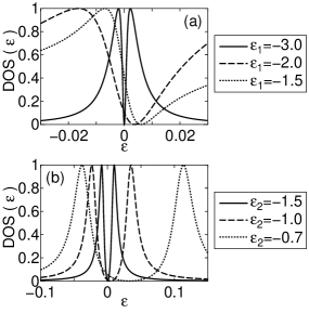
Figure 8: DOS of the dot-1 for the T-shaped DQD ($y=0$): (a) $\varepsilon_{2}=-3.0$ and (b) $\varepsilon_{1}=-3.0$. The inter-dot coupling is chosen as $t_{c}=2.0$.

Figure 8(a) shows the DOS of the dot-1 plotted as a function of $\varepsilon_{1}$. The increase of $\varepsilon_{1}$ causes the broadening of the Kondo resonance and enhances charge fluctuations. Accordingly, the dip structure in DOS of the dot-1 shifts above the Fermi energy and gets more asymmetric. As a result, the conductance gets large with the increase of $\varepsilon_{1}$, as shown in Fig. 9. This is contrasted to the single dot case, where the increase of $\varepsilon_{1}$ decreases the conductance. When the level $\varepsilon_{2}$ of the dot-2 is altered, slightly different behavior appears. In this case the increase of $\varepsilon_{2}$ does not directly enhance charge fluctuations of the dot-1, but mainly increases the renormalized tunneling $\tilde{t}_{c}$ because electron correlations between two dots get somewhat weaker. This merely enlarges the splitting of the double peaks in DOS of the dot-1 (Fig. 8(b)), and thus the conductance is still very small, as seen in the region of $\varepsilon<-1$ in Fig. 9. However, as $\varepsilon_{2}$ approaches the Fermi level, the enhanced $\tilde{t}_{c}$ finally causes charge fluctuations of the dot-1, and then increases the linear conductance. In this way, the gate-voltage control of $\varepsilon_{1}$ and $\varepsilon_{2}$ appears in slightly different ways. Nevertheless, both exhibit a similar tendency in the gate-voltage dependence of the conductance, which is opposite to the single-dot case.

Although we have restricted our discussions to the T-shaped DQD here, similar arguments about the gate-voltage control of the dot levels can be straightforwardly applied to other cases such as the parallel DQD.

To conclude this subsection, we wish to mention some similarities and differences between the present T-shaped DQD and a side-coupled QD that has been studied theoretically Liu ; Kang ; Torio ; Aligia ; Maru and experimentally Sato . In both models, there exists the interference effect due to the T-shaped geometry including the side-coupled QD, which is essential to control transport properties. Namely, the coexistence of a direct tunneling without a side-dot and an indirect tunneling via a side-dot results in an asymmetric transmission probability. In contrast to the T-shaped DQD, where both of the two dots are highly correlated, the side-coupled QD is supposed to have electron correlations only in the side dot. In this sense, we would say that the charge-fluctuation regime with $\varepsilon\sim 0$ in the T-shaped DQD, where electron correlations are somewhat suppressed in the dot-1, may exhibit properties similar to those in the side-coupled QD system.

Figure 9: Linear conductance as a function of the bare energy level: we change $\varepsilon_{1}$ (filled circles), by keeping $\varepsilon_{2}=-3.0$ fixed, while we change $\varepsilon_{2}$ (open circles) by keeping $\varepsilon_{1}=-3.0$ fixed. The inter-dot coupling for these plots is $t_{c}=2.0$. For reference we plot the conductance for the single dot system ($t_{c}=0$) as filled triangles.

III.2.2 spin-polarized leads

We finally discuss the T-shaped DQD connected to the ferromagnetic leads, where the leads $L$ and $R$ have the same orientation of spin-polarization. We will see below that the gate-voltage control discussed above is helpful to understand the characteristic $p$-dependence of the conductance. Here we consider the case of $\varepsilon_{1}=-1.5$, $\varepsilon_{2}=-3.0$ and $t_{c}=2.0$, where the conductance is finite even at $p=0$, as shown in Fig 9.

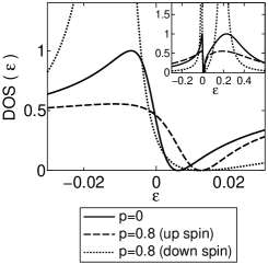
Figure 10: DOS of the dot-1 for the T-shaped DQD: non-polarized leads ($p=0$) and spin-polarized leads ($p=0.8$). We choose $\varepsilon_{1}=-1.5$, $\varepsilon_{2}=-3.0$ and $t_{c}=2.0$. Inset: DOS of the dot-1 drawn in a wider energy range.

Figure 10 shows the DOS of the dot-1 connected to non-polarized leads ($p=0$) and spin-polarized leads ($p=0.8$). The width of the Kondo resonance (with a sharp dip) is changed by the spin-polarization of the leads, so that the DOS of the dot-1 for up-spin (majority spin) electrons is broadened while that for down-spin (minority spin) electrons gets sharp. Accordingly, charge fluctuations of the up-spin (down-spin) electrons are somewhat enhanced (suppressed). Following the analysis done for the gate-voltage control (Fig.9), we naturally expect that the contribution of up-spin (down-spin) electrons to the total conductance gets large (small) under the influence of the spin polarization. We have indeed confirmed this tendency in the conductance, where up-spin (down-spin) currents are increased (decreased) as a function of $p$, as shown in Fig. 11.

Figure 11: Linear conductance as a function of the strength of the spin-polarization $p$. The contribution from up- and down-spin electrons is also shown.

Notice that this result is contrasted to the $p$-dependence in Fig. 5. The difference, as mentioned above, comes from the fact that the double structure of the Kondo resonances is composed of the bonding and anti-bonding Kondo states (the dot-1 and dot-2 Kondo states) in the case of Fig. 5 (Fig. 11), respectively. To see the difference between Figs. 5 and 11 more clearly, we recall that in Fig. 11 the increase of $p$ merely changes the resonance width and thus increases (decreases) $T(\varepsilon=0)$ for up-spin (down-spin) electrons, which results in the linear increase (decrease) of the conductance as a function of $p$. On the other hand, as mentioned before, in the case of Fig. 5, the introduction of $p$ not only changes the width of the asymmetric resonance in $T(\varepsilon)$ but also shifts its peak position for down-spin electrons, which leads to the non-monotonic $p$-dependence of the conductance for down-spin electrons. This consideration clarifies why we have encountered the different $p$-dependence of the conductance in Figs. 5 and 11.

IV Summary

We have studied transport properties of the DQD systems with particular emphasis on the interplay of the Kondo effect and the interference effect. For this purpose we have observed how the Kondo-assisted conductance alters its properties when the system is changed from the serial to parallel geometry, and from the parallel to T-shaped geometry.

For the serial DQD, it is known that the Kondo resonance may have a double-peak structure due to the inter-dot tunneling, which somehow reduces the conductance. In this case, however, there is no interference effect. On the other hand, when the system approaches the parallel DQD, there appear two distinct channels of electron propagation via the bonding and anti-bonding dot states, which respectively form the sharp and broad Kondo resonances. The interference between these two Kondo resonances gives rise to the asymmetric dip structure in the transmission probability, which reduces the conductance significantly. We have seen that the T-shaped DQD exhibits somewhat different properties. In this case, the DOS of the dot-1 connected to the leads has a broader resonance and develops a sharp dip structure in it as a consequence of interference with the dot-2 having a much sharper Kondo resonance. Therefore, the DOS as well as the transmission probability always have the dip structure at the Fermi level, thus giving a very small conductance in the Kondo regime.

It has been shown that the gate-voltage control causes two main effects via the change of the dot-levels: the increase of the dot-level induces charge fluctuations and also causes the renormalization of the effective inter-dot coupling. These effects make the characteristic behavior of the conductance quite different from that for the single dot case. In particular, it has been demonstrated in the T-shaped case that the gate-voltage (i.e. dot-level) control leads to a tendency contrary to the single-dot case: the conductance increases with the increase of the bare level of the dot, reflecting the Kondo effect influenced by the interference effect.

We have also discussed the impact of the FM leads on transport properties. The change in the Kondo resonances due to the spin-polarization of the FM leads modifies the asymmetric structure in the transmission probability, so that the spin-dependent currents may flow depending on the spin-polarization strength $p$. It has been shown that the spin-dependent conductance is quite sensitive to the geometry of DQD, implying that the interference of electrons plays a crucial role to determine the transport properties.

Experimentally, the Kondo effect in DQD systems has been observed recently Jeong ; Chen . It is thus expected that interference effects will be systematically studied in a variety of DQD systems including the T-shaped DQD. We also hope that the spin-dependent conductance in such correlated DQD can be controlled by spin-polarization in the near future.

- (1) D. Goldhaber-Gordon, H. Shtrikman, D. Mahalu, D. Abusch-Magder, U. Meirav, and M. A. Kanster, Nature (London) 391, 156 (1998); D. Goldhaber-Gordon, J. Gres, M. A. Kastner, H. Shtrikman, D. Mahalu, and U. Meirav, Phys. Rev. Lett. 81, 5225 (1998).
- (2) S. M. Cronenwett, T. H. Oosterkamp, and L. P. Kouwenhoven, Science 281, 540 (1998).
- (3) T. K. Ng and P. A. Lee, Phys. Rev. Lett. 61, 1768 (1988).
- (4) L. I. Glazman and M. E. Raikh, JETP Lett. 47, 452 (1988).
- (5) A. Kawabata, J. Phys. Soc. Jpn. 60, 3222 (1991).
- (6) Y. Meir and N. S. Wingreen, Phys. Rev. Lett. 68, 2512 (1992); Y. Meir, N. S. Wingreen, and P. A. Lee, Phys. Rev. Lett. 70, 2601 (1993); A. -P. Jauho, N. S. Wingreen, and Y. Meir, Phys. Rev. B 50, 5528 (1994).
- (7) A. Oguri, H. Ishii, and T. Saso, Phys. Rev. B 51, 4715 (1995).
- (8) For review, see L. P. Kouwenhoven, D. G. Austing, and S. Tarucha, Rep. Prog. Phys. 64, 701 (2001); S. M. Reimann and M. Manninen, Rev. Mod. Phys. 74, 1283 (2002).
- (9) For review, see G. Hackenbroich, Phys. Rep. 343, 463 (2002).
- (10) A. Yacoby, M. Heiblum, D. Mahalu, and H. Shtrikman, Phys. Rev. Lett. 74, 4047 (1995).
- (11) R. Schuster, E. Buks, M. Heiblum, D. Mahalu, V. Umansky, and H. Shtrikman, Nature (London) 385, 417 (1997).
- (12) W. G. van der Wiel, S. De Franceschi, T. Fujisawa, J. M. Elzerman, S. Tarucha, and L. P. Kouwenhoven, Science 289, 2105 (2000).
- (13) Y. Ji, M. Heiblum, D. Sprinzak, D. Mahalu, and H. Shtrikman, Science 290, 779 (2000).
- (14) K. Kobayashi, H. Aikawa, S. Katsumoto and Y. Iye, Phys. Rev. Lett. 88, 256806 (2002).
- (15) W. Izumida, O. Sakai, and Y. Shimizu, J. Phys. Soc. Jpn. 66, 717 (1997).
- (16) R. Lpez, R. Aguado, and G. Platero, Phys. Rev. Lett. 89, 136802 (2002); Phys. Rev. B 69, 235305 (2004).
- (17) D. Boese, W. Hofstetter, and H. Schoeller, Phys. Rev. B 66, 125315 (2002).
- (18) Y. Utsumi, J. Martinek, P. Bruno, and H. Imamura, Phys. Rev. B 69, 155320 (2004).
- (19) G. -M. Zhang, R. L, Z. -R. Liu, and L. Yu, cond-mat/0403629.
- (20) B. Dong, I. Djuric, H. L. Cui, and X. L. Lei, J. Phys: Condens. Matter 16, 4303 (2004).
- (21) Y. Tanaka and N. Kawakami, Proceedings of the International Symposium on Mesoscopic Superconductivity and Spintronics 2004 (World Scientific Publishing) in press.
- (22) J. C. Chen, A. M. Chang, and M. R. Melloch, Phys. Rev. Lett. 92, 176801 (2004).
- (23) T. Aono, M. Eto, and K. Kawamura, J. Phys. Soc. Jpn. 67, 1860 (1998).
- (24) A. Georges and Y. Meir, Phys. Rev. Lett. 82, 3508 (1999).
- (25) R. Aguado and D. C. Langreth, Phys. Rev. Lett. 85, 1946 (2000).
- (26) C. A. Bsser, E. V. Anda, A. L. Lima, M. A. Davidovich, and G. Chiappe, Phys. Rev. B 62, 9907 (2000).
- (27) W. Izumida and O. Sakai, Phys. Rev. B 62, 10260 (2000).
- (28) T. Aono and M. Eto, Phys. Rev. B 63, 125327 (2001).
- (29) R. Sakano and N. Kawakami, Phys. Rev. B 72, 085303 (2005); Journal of Electron Microscopy Supplement (2005) in press.
- (30) H. Jeong, A. M. Chang, and M. R. Melloch, Science 293, 2221 (2001).
- (31) T. -S. Kim and S. Hershfield, Phys. Rev. B 63, 245326 (2001).
- (32) K. Kikoin and Y. Avishai, Phys. Rev. Lett. 86, 2090 (2001); Phys. Rev. B 65, 115329 (2002).
- (33) Y. Takazawa, Y. Imai, and N. Kawakami, J. Phys. Soc. Jpn. 71, 2234 (2002).
- (34) C. A. Bsser, G. B. Martins, K. A. Al-Hassanieh, A. Moreo, and E. Dagotto, Phys. Rev. B 70, 245303 (2004).
- (35) V. M. Apel, M. A. Davidovich, E. V. Anda, G. Chiappe, and C. A. Busser, cond-mat/0404691.
- (36) P. S. Cornaglia and D. R. Grempel, Phys. Rev. B 71, 075305 (2005).
- (37) B. Wang, J. Wang, and H. Guo, J. Phys. Soc. Jpn. 70, 2645 (2001).
- (38) P. Zhang, Q. -K. Xue, Y. Wang, and X. C. Xie, Phys. Rev. Lett. 89, 286803 (2002).
- (39) N. Sergueev, Q. -f. Sun, H. Guo, B. G. Wang, and J. Wang, Phys. Rev. B 65, 165303 (2002).
- (40) J. Ma, B. Dong, and X. L. Lei, cond-mat/0212645.
- (41) R. Lpez and D. Snchez, Phys. Rev. Lett. 90, 116602 (2003).
- (42) J. Knig and J. Martinek, Phys. Rev. Lett. 90, 166602 (2003).
- (43) J. Martinek, Y. Utsumi, H. Imamura, J. Barna, S. Maekawa, J. Knig, and G. Schn, Phys. Rev. Lett. 91, 127203 (2003).
- (44) J. Martinek, M. Sindel, L. Borda, J. Barna, J. Knig, G. Schn, and J. von Delft, Phys. Rev. Lett. 91, 247202 (2003).
- (45) B. Dong, H. L. Cui, S. Y. Liu, and X. L. Lei, J. Phys: Condens. Matter 15, 8435 (2003).
- (46) Y. Tanaka and N. Kawakami, J. Phys. Soc. Jpn. 73, 2795 (2004).
- (47) M. -S. Choi, D. Snchez, and R. Lpez, Phys. Rev. Lett. 92, 056601 (2004).
- (48) A. N. Pasupathy, R. C. Bialczak, J. Martinek, J. E. Grose, L. A. K. Donev, P. L. McEuen, and D. C. Ralph, Science 306, 86 (2004).
- (49) P. Coleman, Phys. Rev. B 29, 3035 (1984).
- (50) A. C. Hewson, The Kondo Problem to Heavy Fermions (Cambridge University Press, Cambridge, 1993).
- (51) M. L. L. de Guevara, F. Claro, and P. A. Orellana, Phys. Rev. B 67, 195335 (2003).
- (52) H. Haug and A. -P. Jauho, in Quantum Kinetics in Transport and Optics of Semi-conductors, ed. M. Cardona et al. (Springer-Verlag, Heidelberg 1998).
- (53) M. Julliere, Phys. Lett. 54A, 225 (1975).
- (54) J. C. Slonczewski, Phys. Rev. B 39, 6995 (1989).
- (55) Y. -L. Liu and T. K. Ng, Phys. Rev. B 61, 2911 (2000).
- (56) K. Kang, S. Y. Cho, J. -J. Kim, and S. -C. Shin, Phys. Rev. B 63, 113304 (2001).
- (57) M. E. Torio, K. Hallberg, A. H. Ceccatto, and C. R. Proetto, Phys. Rev. B 65, 085302 (2002).
- (58) A. A. Aligia and C. R. Proetto, Phys. Rev. B 65, 165305 (2002).
- (59) I. Maruyama, N. Shibata, and K. Ueda, J. Phys. Soc. Jpn. 73, 3239 (2004).
- (60) M. Sato, H. Aikawa, K. Kobayashi, S. Katsumoto, and Y. Iye, cond-mat/0410062