Study of universality crossover in the contact process

Abstract

We consider a generalization of the contact process stochastic model, including an additional autocatalitic process. The phase diagram of this model in the proper two-parameter space displays a line of transitions between an active and an absorbing phase which starts at the critical point of the contact process and ends at the transition point of the voter model. Thus, a crossover between the directed percolation and the compact percolation universality classes is observed at this latter point. We study this crossover by a variety of techniques. Using supercritical series expansions analyzed with partial differential approximants, we obtain precise estimates of the crossover behavior of the model. In particular, we find an estimate for the crossover exponent $\phi=2.00\pm 0.02$. We also show arguments that support the conjecture $\phi=2$.

I Introduction

The phase transitions exhibited by stochastic models with absorbing states have attracted much attention in recent years, particularly in order to identify and understand the aspects which determine the universality classes in those models. Most of these models have not been solved exactly, but a variety of approximations allow quite conclusive results regarding their critical properties. Stochastic models are, of course, well fitted for simulations, but closed form approximations and other analytical approaches have also been useful in investigating their behavior md99 .

One of the simplest and most studied model of this type is the contact process (CP), which was conceived as a simple model for the spreading of an epidemic and proven to display a continuous transition between the absorbing and an active state, even in one dimension h74 . Actually, it was found that the CP is equivalent to other models such as Schlögl’s lattice model for autocatalytic chemical reactions s72 and Reggeon Field Theory (RFT) gt . The CP belongs to the direct percolation (DP) universality class, together with others models such as the Ziff-Gulari-Barshad model of catalysis zgb86 and branching and annihilating walks with an odd offspring tty92 . The DP conjecture states that all phase transitions between an active and an absorbing state in models with a scalar order parameter, short range interactions and no conservation laws belong to this class j81 . This conjecture was verified in all cases studied so far h00 .

Here we study a generalization of the CP, with an additional parameter, so that the CP transition point becomes a critical line. Since the symmetry properties of this generalized model are the same of the CP, it is expected that this critical line should belong to the DP universality class. However, at one point of this line the model is equivalent to the zero temperature Glauber model g63 , also called the voter model l85 , which displays a spin inversion (or particle-hole) symmetry and therefore belongs to another universality class. Thus the critical line in the phase diagram of the generalized model starts at the CP model and ends at the voter model, a crossover between the two universality classes being observed. The voter model belongs to the compact percolation universality class, and also corresponds to a limiting point in the phase diagram of the Domany-Kinzel cellular automaton, where an exact solution is possible dk84 . Thus, the exact critical exponents are known for this model. In a study of models with several absorbing states h97 simulational results are shown for the model we are considering here and a study of the crossover between direct percolation and compact direct percolation may be found in mdh96 , motivated by the possibility to explain the non-universality in models with several absorbing states as a surface effect. Also, the shape of the critical line close to the CDP endpoint in the Domany-Kinzel automaton was studied in detail kt95 ; tikt95 ; ikb01 , and these results are compared to our findings in the conclusion. Some physical motivation for the model we are studying here might be given. In the contact process, the additional term might be understood as an enhancement of the possibility of a sick individual to recover proportional to the number of its first neighbor which are healthy. However, our motivation to study the model is centered on its simplicity and the universality class crossover present in its phase diagram.

In section II we define the model and explain how supercritical series expansions may be obtained for it. The coefficients of the two-variable series for the survival probability up to order 25 are given. Section III contains the description and the results of the Padé and PDA estimates for the model, with emphasis on the multicritical behavior in the voter model limit. Final discussions and the conclusion may be found in section IV.

II Definition of the model and calculation of the coefficients of the supercritical series for the survival probability

The model is defined on a one-dimensional lattice with $N$ sites and periodic boundary conditions. Each site is occupied either by a particle A or a particle B, no holes are allowed. The microscopic state of the model may thus be described by the set of binary variables $\eta=(\eta_{1},\eta_{2},\ldots,\eta_{N})$, where $\eta_{i}=0$ or $1$ if site $i$ is occupied by particles B or A, respectively.

The model evolves in time according to the following Markovian rules:

1. A site $i$ of the lattice is chosen at random.

2. If the site is occupied by a particle B, it becomes occupied by a particle A with a transition rate equal to $p_{a}n_{A}/2$, where $n_{A}$ is the number of A particles in the sites which are first neighbors to site $i$.

3. If site $i$ is occupied by a particle A, it may become occupied by a particle B through two processes:

   • Spontaneously, with a transition rate $p_{c}$.

   • Through an autocatalytic reaction, with a rate $p_{b}n_{B}/2$, where $n_{B}$ is the number of B particles in the sites which are first neighbors to site $i$.

We define the time in such a way the the non-negative parameters $p_{a}$, $p_{b}$, and $p_{c}$ obey the normalization $p_{a}+p_{b}+p_{c}=1$. We may then discuss the behavior of the model in the $(p_{a},p_{c})$ plane without loss of generality.

The probability $P(\eta,t)$ to find the system in state $\eta$ at time $t$ obeys the master equation

$$\frac{\partial P(\eta,t)}{\partial t}=\sum_{i=1}^{N}[w_{i}(\eta^{i})P(\eta^{i},t)-w_{i}(\eta)P(\eta,t)]$$ (1)

where $\eta^{i}$ corresponds to the following configuration

$$\eta^{i}\equiv(\eta_{1},...,1-\eta_{i},...,\eta_{N})$$ (2)

and $w_{i}(\eta)$ is the transition rate of the model, given by

$$w_{i}(\eta)=\frac{\mu}{2}(1-\gamma\eta_{i})\sum_{\delta}\eta_{i+\delta}+\eta_{i},$$ (3)

where $\mu=p_{a}/(1-p_{a})$, $\gamma=(1-p_{c})/p_{a}$, and the sum is over first neighbors of site $i$.

It may be useful to remark that this model may be mapped to a spin system if we describe sites occupied by A and B particles by an Ising spin variables $\sigma_{i}=1$ and $\sigma_{i}=-1$, respectively. In these variables, the transition rate will be given by

$$w_{i}(\sigma)=\frac{\alpha}{2}\left[1+\beta\sigma_{i}-\frac{1}{2}(\epsilon\sigma_{i}+\xi)\sum_{\delta}\sigma_{i+\delta}\right],$$ (4)

where $\alpha=(p_{a}+p_{b}+2p_{c})/2,\beta=(p_{a}-p_{b}-2p_{c})/(pa+p_{b}+2p_{c}),\epsilon=(p_{a}+p_{b})/(p_{a}+p_{b}+2p_{c})$, and $\xi=(p_{a}-p_{b})/(p_{a}+p_{b}+2p_{c})$.

In two particular cases, this model corresponds to well known models. If we make $p_{b}=0$ or $\gamma=1$ contact process is recovered h74 :

$$w_{i}^{(CP)}(\eta)=\frac{\mu}{2}(1-\eta_{i})\sum_{\delta}\eta_{i+\delta}+\eta_{i}.$$ (5)

If now we take $p_{a}=p_{b}$ and $p_{c}=0$ in the spin formulation of the model, the zero temperature linear Glauber model o03 , also known as the voter model, is recovered l85 :

$$w_{i}^{(LGM)}(\sigma)=\frac{\alpha}{2}\left[1-\frac{1}{2}\sigma_{i}\sum_{\delta}\sigma_{i+\delta}\right].$$ (6)

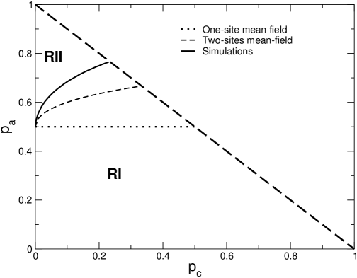
Figure 1: Phase diagram of the model obtained from mean-field approximations and simulations. The physical region is $p_{a}+p_{c}\leq 1$ and the line $p_{a}+p_{c}=1$ corresponds to the contact process. In the region labeled RI the absorbing phase (all particles of type B) is stable, while in the region RII an active phase is stable, with a nonzero density of particles A.

This model has been studied using mean-field approximations dts03 , as well as simulations h97 ; dts03 . For $p_{c}>0$, the stationary state at low values of $p_{A}$ corresponds to the absorbing state, where the density of A particles $\rho_{A}=<N_{A}>/N$ vanishes. As $p_{a}$ is increased, a continuous phase transition occurs and an active stationary state ($\rho_{A}>0$) is stable at high values of $p_{a}$. Thus a critical line is present in the phase diagram starting at $(p_{a}=0.767325(6),p_{c}=1-p_{a}=0.232674(4))$ dj91 (contact process), and ending at $(p_{a}=1/2,p_{c}=0)$ (linear Glauber model), where the transition is discontinuous and between two absorbing states ($\rho_{A}=1$ and $\rho_{B}=1$). In figure 1 results from mean-field calculations and simulations for the phase diagram are shown dts03 . While it is expected that the critical exponents at the whole critical line are the ones of the directed percolation (DP) universality class, a crossover to the compact directed percolation (CDP) universality class exponents happens as $p_{c}$ vanishes h00 . Thus, we may recognize the point $(p_{a}=1/2,p_{c}=0)$ of the phase diagram as a multicritical point. Using supercritical series expansions, for the survival probability, we will study the multicritical singularity in the neighborhood of this point.

Now let us develop a two-variable supercritical series expansion for the model. We follow closely the operator formalism presented in the paper by Jensen and Dickman on series for the CP process and related models dj91 . We may then represent the microscopic configurations of the lattice by the direct product of kets

$$|\eta\rangle=\bigotimes_{i}|\eta_{i}\rangle,$$ (7)

which are defined to be orthonormal

$$\langle\eta|\eta^{\prime}\rangle=\prod_{i}\delta_{\eta_{i},\eta_{i}\prime}.$$ (8)

Now we may define A particles creation and annihilation operators for the site $i$:

$$A_{i}^{\dagger}|\eta_{i}\rangle = (1-\eta_{i})|\eta_{i}+1\rangle,$$

$$A_{i}|\eta_{i}\rangle = \eta_{i}|\eta_{i}-1\rangle.$$ (9)

In this formalism, the state of the system at time $t$ is

$$|\psi(t)\rangle=\sum_{\{\eta\}}p(\eta,t)|\eta\rangle.$$ (10)

If we define the projection onto all possible states as

$$\langle\;|\equiv\sum_{\{\eta\}}\langle\eta|,$$ (11)

the normalization of the state of the system may be expressed as $\langle\;|\psi\rangle=1$. In this notation, the master equation for the evolution of the state of the system (Eq. 1) is

$$\frac{d|\psi(t)\rangle}{dt}=S|\psi(t)\rangle.$$ (12)

The evolution operator $S$ may be expressed in terms of the creation and annihilation operators as $S=\lambda S_{0}+V$ where

$$S_{0} = \sum_{i}[\alpha(2-A_{i-1}^{\dagger}A_{i-1}+A_{i+1}^{\dagger}A_{i+1})+1](A_{i}-A_{i}^{\dagger}A_{i}),$$ (13)

$$V = \sum_{i}(A_{i}^{\dagger}+A_{i}^{\dagger}A_{i}-1)(A_{i-1}^{\dagger}A_{i-1}+A_{i+1}^{\dagger}A_{i+1}),$$ (14)

and the new parameters

$$\lambda\equiv\frac{2p_{c}}{p_{a}}$$

and

$$\alpha\equiv\frac{p_{b}}{2p_{c}}$$

were introduced.

We notice that the operator $S_{0}$ only annihilates A particles (transitions $A\to B$), while the operator $V$ acts in the opposite way, generating transitions $B\to A$. Thus, for small values of the parameter $\lambda$ the creation of A particles is favored, and the decomposition above is convenient for a supercritical perturbation expansion. Let us show explicitly the effect of each operator on a configuration $(\mathcal{C})$.

$$S_{0}({\mathcal{C}})=\alpha\sum_{i}({\mathcal{C}}^{\prime}_{i})+2\alpha\sum_{j}({\mathcal{C}}^{\prime}_{j})+\sum_{k}({\mathcal{C}}^{\prime}_{k})-[\alpha(r_{1}+2r_{2})+r]({\mathcal{C}}),$$ (15)

where the first sum is over the $r_{1}$ sites with A particles and one B neighbor, the second sum is over the $r_{2}$ sites with A particles and two B neighbors and the third sum is over all $r$ sites with A particles of the configuration $(\mathcal{C})$. Configuration $({\mathcal{C}}_{i}^{\prime})$ is obtained replacing the A particle at site $i$ by a B particle. The action of operator $V$ is

$$V({\mathcal{C}})=\sum_{i}({\mathcal{C}}^{\prime\prime}_{i})+2\sum_{j}({\mathcal{C}}^{\prime\prime}_{j})-(q_{1}+2q_{2})({\mathcal{C}}),$$ (16)

where the first sum is over the $q_{1}$ sites with B particles and one A neighbor, the second sum is over the $q_{2}$ sites with B particles and two A neighbors. Configuration $({\mathcal{C}}_{i}^{\prime\prime})$ is obtained replacing the B particle at site $i$ in configuration $(\mathcal{C})$ by a A particle.

To obtain a supercritical expansion for the ultimate survival probability of A particles, we start by remembering that in order to access the long-time behavior of a quantity, it is useful to consider its Laplace transform. For instance, the Laplace transform of the state of the system is

$$|\tilde{\psi}(s)\rangle=\int_{0}^{\infty}e^{-st}|\psi(t)\rangle,$$ (17)

and inserting the formal solution $|\psi(t)\rangle=e^{St}|\psi(0)\rangle$ of the master equation 12, we find

$$|\tilde{\psi}(s)\rangle=(s-S)^{-1}|\psi(0)\rangle.$$ (18)

The stationary state $|\psi(\infty)\rangle\equiv\lim_{t\to\infty}|\psi(t)\rangle$ may then be found noticing that

$$|\psi(\infty)\rangle=\lim_{s\to 0}s|\tilde{\psi}(s)\rangle,$$ (19)

which may be obtained integrating 17 by parts. A perturbative expansion may be obtained assuming that $|\tilde{\psi}(s)\rangle$ may be expanded in powers of $\lambda$ and using 18,

$$|\tilde{\psi}(s)\rangle=|\tilde{\psi}_{0}\rangle+\lambda|\tilde{\psi}_{1}\rangle+\lambda^{2}|\tilde{\psi}_{2}\rangle+\cdots=\frac{1}{s-V-\lambda S_{0}}|\psi(0)\rangle.$$ (20)

Since

$$\frac{1}{s-V-\lambda S_{0}}=\frac{1}{s-V}\left[1+\lambda\frac{1}{s-V}S_{0}+\lambda^{2}\frac{1}{(s-V)^{2}}S_{0}^{2}+\cdots\right],$$ (21)

we arrive at

$$|\tilde{\psi}_{0}\rangle = \frac{1}{s-V}|\psi(0)\rangle$$

$$|\tilde{\psi}_{1}\rangle = \frac{1}{s-V}S_{0}|\tilde{\psi}_{0}\rangle$$ (22)

$$|\tilde{\psi}_{2}\rangle = \frac{1}{s-V}S_{0}|\tilde{\psi}_{1}\rangle$$ (23)

$$\vdots$$

The action of the operator $(s-V)^{-1}$ on an arbitrary configuration $({\mathcal{C}})$ may be found noting that

$$(s-V)^{-1}({\mathcal{C}})=s^{-1}({\mathcal{C}})+\frac{V}{s(s-V)}({\mathcal{C}}),$$ (24)

and using the expression 16 for the action of the operator $V$, we get

$$(s-V)^{-1}({\mathcal{C}})=s_{q}\left\{({\mathcal{C}})+(s-V)^{-1}\left[\sum_{i}({\mathcal{C}}^{\prime\prime}_{i})+2\sum_{j}({\mathcal{C}}^{\prime\prime}_{j})\right]\right\},$$ (25)

where the first sum is over the $q_{1}$ sites with B particles and one A neighbor, the second sum is over the $q_{2}$ sites with B particles and two A neighbors, and we define $s_{q}\equiv 1/(s+q)$, where $q=q_{1}+2q_{2}$.

It is convenient to adopt as the initial configuration a translational invariant one with a single A particle (periodic boundary conditions are adopted). Now we may notice in the recursive expression 25 that the operator $(s-V)^{-1}$ acting on any configuration generates an infinite set of configurations, and thus we are unable to calculate $|\tilde{\psi}\rangle$ in a closed form. We may, however, calculate the extinction probability $\tilde{p}(s)$, which corresponds to the coefficient of the vacuum state $|0\rangle$. As happens also for the models related to the CP studied in dj91 configurations with more than $j$ particles only contribute at orders higher than $j$, and since we are interested in the ultimate survival probability for A particles $P_{\infty}=1-\lim_{s\to 0}s\tilde{p}(s)$, $s_{q}$ may be replaced by $1/q$ in Eq. 25. To illustrate the procedure, we will perform the explicit calculation of the series for $\lim_{s\to 0}s\tilde{p}(s)$ up to third order in $\lambda$. We furthermore represent a configuration denoting by $\bullet$ a site occupied by an A particle and by $\circ$ a site occupied by a B particle. Thus $(\bullet\circ\bullet)$ denotes the translationally invariant configuration $\sum_{i}A_{i}^{\dagger}A_{i+2}^{\dagger}|0\rangle$. The B particles situated to the left of the leftmore A particle in a configuration and the ones situated to the right of the rightmost A particle are omitted in the representation of this configuration. The vacuum state will be represented by $(0)$. As stated above, at $t=0$ the system will be supposed to be in the configuration $|\psi(0)\rangle=\sum_{i}A_{i}^{\dagger}|0\rangle=(\bullet)$. Keeping configurations with up to three particles, and omitting the global factor $1/s$, the first of the recursion relations Eqs. 22 leads to

$$|\tilde{\psi}_{0}\rangle=\frac{1}{2}[(\bullet)+(\bullet\bullet)+(\bullet\bullet\bullet)+\cdots].$$ (26)

The next step is the calculation of $|\tilde{\phi}_{0}\rangle=S_{0}|\tilde{\psi}_{0}\rangle$. Now we need to keep only configurations with up to two particle. The result is

$$|\tilde{\phi}_{0}\rangle=\frac{1}{2}[(2\alpha+1)(0)+(\bullet)+\bullet\circ\bullet)+\cdots].$$ (27)

Now we obtain $|\tilde{\psi}_{1}\rangle=(s-V)^{-1}|\tilde{\phi}_{0}\rangle$ for $s=0$, resulting in

$$|\tilde{\psi}_{1}\rangle=\frac{1}{2}(2\alpha+1)(0)+\frac{1}{4}(\bullet)+\frac{1}{4}(\bullet\bullet)+\frac{1}{8}(\bullet\circ\bullet)+\cdots.$$ (28)

From this point on we will only show the results of each step, up to the relevant numbers of A particles:

$$|\tilde{\phi}_{1}\rangle = \frac{1}{4}(2\alpha+1)(0)+\frac{1}{4}(2\alpha+2)(\bullet)+\cdots,$$

$$|\tilde{\psi}_{2}\rangle = \frac{1}{4}(2\alpha+1)(0)+\frac{1}{8}(2\alpha+2)(\bullet)+\cdots,$$

$$|\tilde{\phi}_{2}\rangle = \frac{1}{8}(2\alpha+2)(2\alpha+1)(0)+\cdots,$$

$$|\tilde{\psi}_{3}\rangle = \frac{1}{8}(2\alpha+2)(2\alpha+1)(0)+\cdots.$$

The first coefficients of the ultimate survival probability will then be given by

$$P_{\infty}=1-\frac{1}{2}(2\alpha+1)\lambda+-\frac{1}{4}(2\alpha+1)\lambda^{2}+\frac{1}{8}(2\alpha+2)(2\alpha+1)\lambda^{3}+\cdots$$ (29)

The algebraic operations above may be easily performed in a computer using a proper algorithm. The configurations are expressed as binary numbers and the coefficients as double precision variables. Although we have tried to do the calculation representing the coefficients as rational numbers, thus avoiding any roundoff errors since all calculations were done with integers, we found that the denominators increase very rapidly with the order of the calculations, and thus we were unable to perform the calculations this way up to a reasonable order. With rather modest computational resources (Athlon MP2200, double processor, 1Gb memory) it is not difficult to calculate the coefficients up to order 25. The required processing time amounts to about 6 hours, the limiting factor is actually the memory required for the calculation. The maximum number of terms (polynomials in $\alpha$) amounts to more than $44\times 10^{6}$. We define the coefficients $b_{i,j}$ as:

$$P_{\infty}=1-\frac{1}{2}(2\alpha+1)\lambda-\sum_{i=2}^{25}\sum_{j=0}^{i-1}b_{i,j}\lambda^{i}\alpha^{j},$$ (30)

and they are listed in Table 1. Up to order 24, our results are numerically coincident with the supercritical series expansion for the ultimate survival probability of the contact process dj91 , in the particular case $\alpha=0$ (we remark that the variable $\lambda$ in the supercritical expansion for the ultimate survival probability in reference dj91 is half the variable $\lambda$ we use here).

III Analysis of the series

Let us consider initially the one variable series for fixed values of $\alpha$

$$P_{\infty}=\sum_{i=0}^{25}a_{i}(\alpha)\lambda^{i}.$$ (31)

As a preliminary test, we may apply the ratio method g89 to these series. The results for $r_{i}=a_{i}/a_{i-1}$ as functions of $1/i$ are depicted in Figure 2. In the case $\alpha=0$ (circles), the asymptotic linear behavior $r_{i}\approx 1,6489(1-0.7231/i)$, obtained from precise estimates for $\lambda_{c}$ and the exponent $\beta$ for the contact process dj91 . In the figure it is apparent that the ratios approach the asymptotic limit as $i$ is increased, as a matter of fact this approach is close to linear in $1/i$. Thus, we may infer that for this model the singularity which is closer to the origin is actually the physical singularity. As the value of $\alpha$ is increased, one may notice that the asymptotic linear behavior in $1/i$ for the ratios occurs only for higher values of $i$, and thus it will be increasingly difficult to obtain precise estimates for higher values of $\alpha$.

Even in cases where the singularity of physical interest is the one closest to the origin, the d-log Padé approximants usually lead to better estimates than the ratio method g89 . The approximants are defined as ratios of two polynomials $P_{L}(\lambda)$ and $Q_{M}(\lambda)$:

$$F_{LM}(\lambda)=\frac{P_{L}(\lambda)}{Q_{M}(\lambda)}=\frac{\sum_{i=0}^{L}p_{i}\lambda^{i}}{1+\sum_{j=1}^{M}q_{j}\lambda^{j}}.$$ (32)

The series for $\frac{d}{d\lambda}\ln P_{\infty}(\lambda)$ for fixed values of $\alpha$ are substituted in the defining equation 32 and the coefficients of the polynomials are chosen such that the identity is true up to the order of the available series expansion. Thus approximants with $L+M\leq 24$ may be built with the available series. Usually diagonal ($L=M$) or close to diagonal approximants furnish better results, so we restricted our calculations to these cases. The estimate for the critical value of $\lambda$ is found among the poles of the approximant, the estimate for the critical exponent $\beta$ will be the residue at this pole.

We thus built approximants with $\alpha$ ranging between 0 and 40, estimating the critical value of the parameter $\lambda$ as well as the critical exponent $\beta$. Although for small values of $\alpha$ the results are very good, with estimates of $\beta$ comparable to the best ones in the literature for the contact process, as the value of $p_{c}$ is decreased we notice a growing dispersion of the estimates for the exponent and for $p_{c}<0.01$ most of the approximants lead even to ill conditioned systems of linear equations for the coefficients, and therefore we were not able to obtain estimates in this region. We made additional one-variable investigations, such as obtaining approximants for $(\lambda_{c}-\lambda)\frac{d}{d\lambda}P_{s}(\lambda)=\beta$ for several values of $\lambda_{c}$ and searching for the intercept of the curves $\beta(\lambda_{c})$ dj91 and non-homogeneous Padé approximants g89 ; nha , and although some improvements of the estimates may be obtained in certain cases, the situation does not change qualitatively. In figure 3 the Padé estimates for the critical line are displayed.

Actually, the increasing dispersion of the estimates as the parameter $p_{c}$ approaches zero is not a surprise, since as was mentioned above in this limit the model corresponds to the voter model which is in the compact directed percolation (CDP) universality class, whose exponents are different from the ones of the contact process, which belongs to the directed percolation (DP) universality class. For the voter model, the exponent $\beta$ of the order parameter is equal to zero (a discontinuity in the order parameter occurs at the transition) h00 , but the exponent for the survival probability $\beta^{\prime}$ is distinct from $\beta$ and equal to 1 dt95 . Therefore a crossover to from the DP to the CDP universality class occurs as $p_{c}\to 0$, and it is known that in such situations the reduction of two-variable series to one variable leads to very poor estimates fk77 . So we analyzed the series without reducing the problem to one variable, and to our knowledge the best results for two-variable series applied to multicritical phenomena in the literature were obtained using the partial differential approximants (PDA’s) fk77 . They may be regarded as a generalization to two variables of the d-log Padé approximants. The defining equation of the approximants is

$$P_{\mathbf{L}}(x,y)F(x,y)=Q_{\mathbf{M}}(x,y)\frac{\partial F(x,y)}{\partial x}+R_{\mathbf{N}}(x,y)\frac{\partial F(x,y)}{\partial y},$$ (33)

where $P$, $Q$, and $R$ are polynomials in the variables $x$ and $y$ with the set of nonzero coefficients ${\mathbf{L}}$, ${\mathbf{M}}$, and ${\mathbf{N}}$, respectively. The coefficients of the polynomials are obtained through substitution of the series expansion for the quantity which is going to be analyzed

$$f(x,y)=\sum_{k,k^{\prime}=0}f(k,k^{\prime})x^{k}y^{k^{\prime}}$$ (34)

into the defining equation 33 and requiring the equality to hold for a set of indexes defined as ${\mathbf{K}}$. Again this procedure leads to a system of linear equations for the coefficients of the polynomials, and since the coefficients $f_{k,k^{\prime}}$ of the series are known for a finite set of indexes this sets an upper limit to the number of coefficients in the polynomials. Since the number of equations has to match the number of unknown coefficients, we must have that the numbers of elements in each set satisfy $K=L+M+N-1$ (one coefficient is fixed arbitrarily). An additional issue, which is not present in the one-variable case, is the symmetry of the polynomials. Two frequently used options are the triangular and the rectangular arrays of coefficients. The choice of these symmetries is related to the symmetry of the series itself s90 . Below we discuss the solution we adopted in the present case for this point.

Let us suppose that quantity represented by the series is expected to have a multicritical behavior at a point $(x_{c},y_{c})$, described by

$$f(x,y)\approx|\Delta\widetilde{x}|^{-\gamma}Z\left(\frac{|\Delta\widetilde{y}|}{|\Delta\widetilde{x}|^{\phi}}\right),$$ (35)

where

$$\Delta\widetilde{x}=(x-x_{c})-(y-y_{c})/e_{2},$$ (36)

and

$$\Delta\widetilde{y}=(y-y_{c})-e_{1}(x-x_{c}).$$ (37)

Here $\gamma$ is the critical exponent of the quantity described by $f$ when $\Delta\widetilde{y}=0$, $e_{1}$ and $e_{2}$ are the scaling slopes fk77 and $\phi$ is the crossover exponent. The function $Z(z)$ is singular for one or more values of its argument, corresponding to the critical line(s) incident on the multicritical point. Once the coefficients of the defining polynomials are obtained, the estimated location of the multicritical point corresponds to the common zero of the polynomials $Q_{M}$ and $R_{N}$. This may be seen substituting the scaling form 35 in the defining equation 33 of the approximant. The exponents and scaling slopes may also be obtained directly from the polynomials, without integrating the partial differential equation. A detailed discussion of the algorithm, as well as computer codes, may be found in s90 .

Before proceeding with the analysis of the series, it is convenient to perform a change of variables, since the multicritical point in the original variables is located at $\alpha\to\infty$. We thus express the series in the variables

$$x=\lambda=\frac{2p_{c}}{p_{a}}$$

$$y=\alpha\lambda=\frac{1-p_{a}-p_{c}}{p_{a}}.$$

In these new variables the multicritical point is located at $x=0$, $y=1$, and the survival probability may be written as

$$P_{\infty}=1-\frac{1}{2}x-y-xF(x,y),$$ (38)

where

$$F(x,y)=\sum_{i=1}^{24}\sum_{j=0}^{i}b_{i+1,j}x^{i-j}y^{j}$$ (39)

is represented by a series with triangular symmetry, which is very convenient to be analyzed using PDA’s. The number of approximants which may be obtained from the series is very big, so we restricted ourselves to approximants with the number of elements in $\mathbf{M}$ close to the number of elements in $\mathbf{N}$. The polynomials had the same triangular symmetry as the series, but in most cases some higher order elements of the polynomials were set equal to zero in order to match the number of unknowns to the number of equations in the set of linear equations for the coefficients. This is a rather standard procedure and is discussed in detail by Styer s90 . Even at rather low orders, we found a reasonable agreement between most of the estimates from different approximants. Finally, we considered a set of 42 approximants which use the elements of the series for $F(x,y)$ with highest orders $i$ between 15 and 24. Discarding some approximants which generated estimates which were rather far away of the general trend, finally we used a set of 36 approximants to obtain the estimates.

In figure 4 the estimates for the location of the multicritical point are displayed. We notice that the estimates are very close to the exactly known values $x=0$ and $y=1$. The estimated values for $x_{c}$ and $y_{c}$ are $(0.4\pm 1.8)\times 10^{-6}$ and $y=1.0000\pm 0.0003$. The exponent $-\gamma$ in the multicritical scaling form 35 corresponds to the exponent $\beta^{\prime}$ of the CDP universality class. The estimated value is equal to $1.00\pm 0.01$, which agrees very well with the exact value $\beta^{\prime}=1$ h00 . Finally, the crossover exponent was estimated as $\phi=2.01\pm 0.03$, and thus the mean field value for this exponent ($\phi=2$ dts03 ) is within the confidence interval of our estimate. The estimates for $\beta^{\prime}$ and $\phi$ are shown in figure 5. We also obtained biased PDA’s, fixing the other parameters at their known values and calculating improved estimates for $\phi$. This procedure resulted in the estimate $\phi=2.00\pm 0.02$. We thus conclude that our estimates for $\phi$ are very close to the classical value of the crossover exponent. The estimates for the slopes of the scaling axes show a rather broad distribution, a significant majority of the approximants provide quite large values for $e_{1}$, while $e_{2}$ is typically much smaller. This suggests that $\Delta\widetilde{y}=x$ and it is reasonable to choose $\Delta\widetilde{x}=1-y$, since it corresponds to the weak direction, parallel to the critical line at the multicritical point. In the limit of the voter model ($x=0$) we notice that the series 38 reduces to the exact result $P_{\infty}=1-y$.

One way to actually estimate values of the quantity which is described by a PDA is to integrate the equation using the method of characteristics. A timelike variable $\tau$ is defined and a family of curves $(x(\tau),y(\tau))$ (the characteristics) is considered. These curves are defined by the equations

$$\frac{dx}{d\tau} = Q_{M}(x(\tau),y(\tau)),$$

$$\frac{dy}{d\tau} = R_{N}(x(\tau),y(\tau)).$$ (40)

Along such a curve, the defining equation of the PDA 33 leads to an ordinary differential equation for $F$.

$$\frac{dF}{d\tau}=P_{L}(x(\tau),y(\tau))F,$$ (41)

which may readily be integrated, providing the value of $F$ at the points of the characteristics, once we know this value at a initial point. Our efforts to obtain estimates for the survival probability, particularly close to the multicritical point, using this procedure were not very successful. Nevertheless, it is worth to mention that an estimate for the critical line may be obtained this way. The critical line, which connects the point which corresponds to the CP to the multicritical point of the voter model transition is a line of singularities, and it is not difficult to show that such a line is one of the characteristics defined by equations 40. Therefore, the characteristic whose initial point is located on the transition point of the CP, which is known with great accuracy, is an estimate for the critical line. We therefore chose a particular approximant with estimates close to the mean values. The number of elements in the sets for this approximant are $K=300$, $L=171$, and $M=N=65$. In figure 3 this characteristic curve is shown, and a nice agreement with other estimates of the critical line may be observed.

IV Conclusion and discussion

We may notice that the coefficients $b(i,i-1)$, for $i=1,2,\ldots$ are equal to $1/2$, a result which is indicated by the coefficients below but may be shown to be true in general using the operator formalism above. Therefore, we may sum these set of terms in the series, obtaining

$$P_{\infty}=(1-y)\left[1-\frac{1}{2}\frac{x}{(1-y)^{2}}-\ldots\right].$$ (42)

Now if we compare this expression with the multicritical scaling form 35, we may recognize between braces the two first terms of a Taylor expansion of the multicritical scaling function $Z(z)$, where the variable $z$ is identified as $\frac{x}{(1-y)^{2}}$. This agrees with the estimates obtained from the PDA’s. Moreover, remembering that for $y=0$ the series represents the CP, the function $Z(z)$ may be recognized as the survival probability of the CP, which was studied in great detail dj91 and found to have a singularity at $z_{0}=0.6064$ with the exponent $\beta^{\prime}=\beta=0.276486$. As expected, the critical line is characterized by the same exponent of the CP, that is, is in the DP universality class. The critical line corresponds to $z=z_{0}$, that is

$$x=z_{0}(1-y)^{2},$$ (43)

and this curve is shown in figure 3. It is interesting to notice that the agreement of this estimate of the critical line with the other two, obtained from Padé and partial differential approximants, is quite good even far away from the multicritical point. The multicritical scaling form with the identification of the scaling variable $z$ above is exact in the limit $p_{c}=0$ (biased voter model) and reproduces the supercritical series expansion for the CP, when $y=0$. It does, however, not reproduce the two-variable supercritical series expansion for the full model we considered here away from these limiting cases.

The Domany Kinzel probabilistic cellular automaton dk84 in part of its two-dimensional phase diagram corresponds to a synchronous update version of the contact process, and as stated above has the synchronous update voter model as a endpoint of the critical line. It is believed, although to our knowledge not proven, that if in a particular model the update procedure is changed from synchronous to asynchronous, the critical exponents do not change.Some bounds for the critical line are presented in kt95 . Although an upper bound for this line due to Liggett l94 is quadratic close to the CDP endpoint, the lower bounds are linear, and thus the asymptotic behavior of the critical line is not fixed by those bounds. The critical line is studied in more detail by simulations and series expansions in tikt95 , and based on this results the authors conjectured a quadratic asymptotic behavior of the critical line, consistent with $\phi=2$.Finally, a more detailed series analysis is done in ikb01 , but since one-variable Padé approximants were used, the results are not precise in the region close to the CDP point. Thus, there are indications that the crossover exponent has the same value in both models, and if these indications are correct, the invariance of this multicritical exponent with respect to the update procedure is verified in this particular case.

In conclusion, the analysis of the series for the ultimate survival probability using PDA’s lead to quite precise estimates for the multicritical exponents, and these estimates, together with the possibility to sum the terms of the two-variable series which are linear in $x$ allowed us to conjecture the exact form of the multicritical scaling expression. The multicritical scaling function $Z(z)$ is known as a series expansion up to order 25.

$i$	$j$	$b_{i,j}$
1	1	0.10000000000000000000D+01
1	0	0.50000000000000000000D+00
2	1	0.50000000000000000000D+00
2	0	0.25000000000000000000D+00
3	2	0.50000000000000000000D+00
3	1	0.75000000000000000000D+00
3	0	0.25000000000000000000D+00
4	3	0.50000000000000000000D+00
4	2	0.15000000000000000000D+01
4	1	0.11875000000000000000D+01
4	0	0.28125000000000000000D+00
5	4	0.50000000000000000000D+00
5	3	0.25000000000000000000D+01
5	2	0.35234375000000000000D+01
5	1	0.18867187500000000000D+01
5	0	0.34375000000000000000D+00
6	5	0.50000000000000000000D+00
6	4	0.37500000000000000000D+01
6	3	0.81665039062499928945D+01
6	2	0.73991699218749946709D+01
6	1	0.29899902343749985789D+01
6	0	0.44726562499999982236D+00
7	6	0.50000000000000000000D+00
7	5	0.52499999999999982236D+01
7	4	0.16280639648437500000D+02
7	3	0.21964294433593751776D+02
7	2	0.14622192382812501776D+02
7	1	0.47470703125000008881D+01
7	0	0.60223388671874964472D+00
8	7	0.50000000000000000000D+00
8	6	0.69999999999999982236D+01
8	5	0.29241512298583977269D+02
8	4	0.54546823501586914062D+02
8	3	0.52912919998168961299D+02
8	2	0.27873636245727544391D+02
8	1	0.75799846649169939638D+01
8	0	0.83485031127929723027D+00
9	8	0.50000000000000000000D+00
9	7	0.90000000000000017763D+01
9	6	0.48670531988143883594D+02
9	5	0.11948751342296599631D+03
9	4	0.15729669463192959000D+03
9	3	0.11890031438403647712D+03
9	2	0.51820946525644346891D+02
9	1	0.12126680864228140954D+02
9	0	0.11814667913648822050D+01
10	9	0.50000000000000000000D+00
10	8	0.11249999999999982236D+02
10	7	0.76407402418553784784D+02
10	6	0.23825064151361545761D+03
10	5	0.40643453331768384373D+03
10	4	0.41173626079900831342D+03
10	3	0.25488795003760951196D+03
10	2	0.94770005067848632762D+02
10	1	0.19463028091937289332D+02
10	0	0.16988672076919923981D+01

11	10	0.50000000000000000000D+00
11	9	0.13750000000000004440D+02
11	8	0.11453289534710346941D+03
11	7	0.44150459107663433400D+03
11	6	0.94395713065082347270D+03
11	5	0.12251638531684152511D+04
11	4	0.10067004627495166335D+04
11	3	0.52744546391776081506D+03
11	2	0.17102490738153186100D+03
11	1	0.31313301122887615690D+02
11	0	0.24775957118665874467D+01
12	11	0.50000000000000000000D+00
12	10	0.16500000000000039079D+02
12	9	0.16534952380310286024D+03
12	8	0.77136775289458459070D+03
12	7	0.20158736418235778664D+04
12	6	0.32476491678046719435D+04
12	5	0.33907974883298468427D+04
12	4	0.23413097838386356386D+04
12	3	0.10630662385637921207D+04
12	2	0.30555868520944353683D+03
12	1	0.50452588505226367843D+02
12	0	0.36488812342264482779D+01
13	12	0.50000000000000000000D+00
13	11	0.19499999999999982236D+02
13	10	0.23139824792517162954D+03
13	9	0.12840079302994218402D+04
13	8	0.40209683861219263079D+04
13	7	0.78496665288886928735D+04
13	6	0.10096110998534653102D+05
13	5	0.88003157466952828258D+04
13	4	0.52368347467192908339D+04
13	3	0.20980007339714172864D+04
13	2	0.54172526170510240106D+03
13	1	0.81489527352144666139D+02
13	0	0.54293656084851633636D+01
14	13	0.49999986588954925537D+00
14	12	0.22749997384846243342D+00
14	11	0.31544379761375296311D+03
14	10	0.20523899291719041038D+04
14	9	0.75794568674053097723D+04
14	8	0.17597122905598574504D+05
14	7	0.27244155488205645809D+05
14	6	0.29082737294330742727D+05
14	5	0.21732772717178829857D+05
14	4	0.11357034171626549934D+05
14	3	0.40697753516544512564D+04
14	2	0.95363664836240946698D+03
14	1	0.13169793741584487900D+03
14	0	0.81325422193071297272D+01

15	14	0.50000000000000000000D+00
15	13	0.26249998256564137655D+02
15	12	0.42048775894871077696D+03
15	11	0.31693914938186833474D+04
15	10	0.13620079986016961903D+05
15	9	0.37037632746719575393D+05
15	8	0.67783286393305548500D+05
15	7	0.86632679492839894663D+05
15	6	0.78910368357158162666D+05
15	5	0.51571902934753062197D+05
15	4	0.24020987390678723016D+05
15	3	0.77874939092949517771D+04
15	2	0.16707029021016392533D+04
15	1	0.21330513440327356633D+03
15	0	0.12275012836144905126D+02
16	15	0.50000000000000000000D+00
16	14	0.29999999329447643248D+02
16	13	0.54975682655068318638D+03
16	12	0.47510546519798584341D+04
16	11	0.23493882045888385690D+05
16	10	0.73897182789227748855D+05
16	9	0.15755031904987298219D+06
16	8	0.23687090513090347521D+06
16	7	0.25718644037330271601D+06
16	6	0.20406058122209760341D+06
16	5	0.11843376024372214061D+06
16	4	0.49739262723985895320D+05
16	3	0.14718788444797093362D+05
16	2	0.29113789219292591781D+04
16	1	0.34558659823607458250D+03
16	0	0.18620961415130533822D+02
17	16	0.50000000000000000000D+00
17	15	0.33999999329447789797D+02
17	14	0.70671335354464535072D+03
17	13	0.69402158602317101099D+04
17	12	0.39112396145099372901D+05
17	11	0.14079076808597497105D+06
17	10	0.34548310262719810204D+06
17	9	0.60241714803092252239D+06
17	8	0.76636402935447742734D+06
17	7	0.72224826262886052674D+06
17	6	0.50729839736110484693D+06
17	5	0.26473279696452087783D+06
17	4	0.10122975226631107936D+06
17	3	0.27555943803143052583D+05
17	2	0.50567133817482794455D+04
17	1	0.56084260997641584012D+03
17	0	0.28405733950687368505D+02

18	17	0.50000000000000000000D+00
18	16	0.38249999329447760487D+02
18	15	0.89504578674400576687D+03
18	14	0.99102626626136949283D+04
18	13	0.63122994123535232091D+05
18	12	0.25768737165396164989D+06
18	11	0.72043302015833452500D+06
18	10	0.14399790608479312581D+07
18	9	0.21166673049189457245D+07
18	8	0.23292641415436174945D+07
18	7	0.19371723268429082764D+07
18	6	0.12198708033512473125D+07
18	5	0.57806709777733367161D+06
18	4	0.20284284513882400169D+06
18	3	0.51115204972041548003D+05
18	2	0.87477997069442139377D+04
18	1	0.91057218719788650673D+03
18	0	0.43520782874229171355D+02
19	18	0.49999999999999911182D+00
19	17	0.42749999329447687657D+02
19	16	0.11186774875974003773D+04
19	15	0.13869278218084735243D+05
19	14	0.99114912109387987015D+05
19	13	0.45525829782828974856D+06
19	12	0.14375483791065075678D+07
19	11	0.32614349098596422393D+07
19	10	0.54767322733604206774D+07
19	9	0.69423928844342714938D+07
19	8	0.67230154917519895363D+07
19	7	0.50002124204980198385D+07
19	6	0.28527370161475179344D+07
19	5	0.12379379646484691690D+07
19	4	0.40134571279240418562D+06
19	3	0.94145168822797273833D+05
19	2	0.15093606456186623887D+05
19	1	0.14798263077956907984D+04
19	0	0.66930218067927942371D+02
20	19	0.50000000000000000000D+00
20	18	0.47499999329447701867D+02
20	17	0.13817585309510260671D+04
20	16	0.19064302620655780629D+05
20	15	0.15187519641466302289D+06
20	14	0.77950921221482092349D+06
20	13	0.27591465361185987248D+07
20	12	0.70457626117426288558D+07
20	11	0.13386942665323722234D+08
20	10	0.19328829379718762027D+08
20	9	0.21502873943167273296D+08
20	8	0.18574978781954090578D+08
20	7	0.12487211289613961984D+08
20	6	0.65099543472194438820D+07
20	5	0.26049731385271019945D+07
20	4	0.78478644916613982118D+06
20	3	0.17219353528307646428D+06
20	2	0.25969733685492251140D+05
20	1	0.24071073326750083154D+04
20	0	0.10337399908888862398D+03

21	20	0.49999999999999955591D+00
21	19	0.52499999329447701867D+02
21	18	0.16886733349218010502D+04
21	17	0.25785991340403939808D+05
21	16	0.22768166104993685650D+06
21	15	0.12978288769859755902D+07
21	14	0.51154797613905129693D+07
21	13	0.14596468511940512868D+08
21	12	0.31124330624461475913D+08
21	11	0.50710951504426553526D+08
21	10	0.64100799162967723177D+08
21	9	0.63467922470529245515D+08
21	8	0.49453964458225394551D+08
21	7	0.30321310892616786247D+08
21	6	0.14550387399195248150D+08
21	5	0.54012506504483805969D+07
21	4	0.15195548211633345125D+07
21	3	0.31313135707735888502D+06
21	2	0.44571407092920996007D+05
21	1	0.39157750249797601327D+04
21	0	0.15998830271630990473D+03
22	21	0.50000000000000088817D+00
22	20	0.57749999329447438967D+02
22	19	0.20440335494663091076D+04
22	18	0.34373382551268485407D+05
22	17	0.33466104195644446051D+06
22	16	0.21070967788898307126D+07
22	15	0.91945254038400960894D+07
22	14	0.29128975460417066756D+08
22	13	0.69213935104954478205D+08
22	12	0.12623609387336516274D+09
22	11	0.17963375603295976823D+09
22	10	0.20164422581600076611D+09
22	9	0.17971976143434213568D+09
22	8	0.12747436997852454876D+09
22	7	0.71815965145384188517D+08
22	6	0.31918963164481914951D+08
22	5	0.11049035068083481458D+08
22	4	0.29157961094487756525D+07
22	3	0.56650954312689849601D+06
22	2	0.76372602458216514165D+05
22	1	0.63802269924577696968D+04
22	0	0.24876519640924477094D+03

23	22	0.50000015522128578027D+00
23	21	0.63250003986086227314D+02
23	20	0.24526847667386335594D+04
23	19	0.45219068649736344767D+05
23	18	0.48319032233047343183D+06
23	17	0.33439431430492136954D+07
23	16	0.16069927289546637183D+08
23	15	0.56208076057486060506D+08
23	14	0.14791153728125157051D+09
23	13	0.29990967758279261090D+09
23	12	0.47669571268868358160D+09
23	11	0.60118669013109657939D+09
23	10	0.60634053785517059154D+09
23	9	0.49107989528314268667D+09
23	8	0.31953776898326688993D+09
23	7	0.16647521279074794620D+09
23	6	0.68894669993720274447D+08
23	5	0.22337519908203442575D+08
23	4	0.55496488699702037905D+07
23	3	0.10196528668928661609D+07
23	2	0.13050250676997474652D+06
23	1	0.10386065610378922841D+05
23	0	0.38696067609363534955D+03
24	23	0.49999999999999706901D+00
24	22	0.69000000457884933524D+02
24	21	0.29197000139992891121D+04
24	20	0.58774468615505739421D+05
24	19	0.68638127471201864082D+06
24	18	0.51981592602471167197D+07
24	17	0.27383018956536124832D+08
24	16	0.10521292804690998146D+09
24	15	0.30494730611982263646D+09
24	14	0.68324606257180731105D+09
24	13	0.12048047382312678799D+10
24	12	0.16938688975594596186D+10
24	11	0.19158522496513690214D+10
24	10	0.17528882189096098187D+10
24	9	0.13003099701647686803D+10
24	8	0.78129739240902704722D+09
24	7	0.37851359502279247060D+09
24	6	0.14654979817717892487D+09
24	5	0.44688725216130675832D+08
24	4	0.10490868838890698988D+08
24	3	0.18288174674782467832D+07
24	2	0.22289668577994086184D+06
24	1	0.16948463518651144532D+05
24	0	0.60509199550607846163D+03

25	24	0.50000051317104317050D+00
25	23	0.75000019616897146690D+02
25	22	0.34503863852011384949D+04
25	21	0.75555516468201169288D+05
25	20	0.96061396122189321999D+06
25	19	0.79292390146647733217D+07
25	18	0.45593449242937929000D+08
25	17	0.19157385641492643557D+09
25	16	0.60860240979789494986D+09
25	15	0.14987944522389162749D+10
25	14	0.29148047590757961700D+10
25	13	0.45381694251898121450D+10
25	12	0.57125179306761664221D+10
25	11	0.58520654724976619576D+10
25	10	0.48967910880832077324D+10
25	9	0.33495648941633358042D+10
25	8	0.18689764057712466183D+10
25	7	0.84597759965914463009D+09
25	6	0.30764609873623349756D+09
25	5	0.88524517163033653588D+08
25	4	0.19689926825686265843D+08
25	3	0.32638605561858318182D+07
25	2	0.37947216762104512000D+06
25	1	0.27603268426234146559D+05
25	0	0.94519638900755200694D+03

Table 1: Coefficients $b_{i,j}$ of the supercritical series expansion for the ultimate survival probability of A particles.

Figure 2: Ratio of successive coefficients of the series expansion in $\lambda$ for fixed values of $\alpha$. The results shown are for $\alpha=0$ (circles), $\alpha=1$, $\alpha=2$, $\alpha=3$ $\alpha=5$, and $\alpha=10$ (triangles pointing down). The solid line shows the expected asymptotic behavior for $\alpha=0$ (contact process).

Figure 3: Estimates for the critical line. Curve (a) shows results from simulations (triangles) and Padé approximants (circles). Curve (b) displays the characteristic which starts at the CP (full line) and simulation results (triangles). In curve (c) the full line is again the characteristic and the values which follow from the multicritical scaling form are represented by crosses.

Figure 4: Estimates for the location of the multicritical point provided by the set of PDA’s.

Figure 5: Estimates for the values of the exponents $\beta^{\prime}$ and $\phi$.