Gutzwiller variational theory for the Hubbard model with attractive interaction

Abstract

We investigate the electronic and superconducting properties of a negative-$U$ Hubbard model. For this purpose we evaluate a recently introduced variational theory based on Gutzwiller-correlated BCS wave functions. We find significant differences between our approach and standard BCS theory, especially for the superconducting gap. For small values of $|U|$, we derive analytical expressions for the order parameter and the superconducting gap which we compare to exact results from perturbation theory.

1 Introduction

Gutzwiller-correlated wave functions [1] were originally proposed for a variational examination of the one-band Hubbard model [2]

$$\hat{H}=\sum_{i\neq j}\sum_{\sigma=\uparrow,\downarrow}t_{i,j}\hat{c}_{i\sigma}^{+}\hat{c}_{j\sigma}+U\sum_{i}\hat{n}_{i\uparrow}\hat{n}_{i\downarrow}=\hat{H}_{\rm kin}+\hat{H}_{U}$$ (1)

with positive Coulomb repulsion $U$. Here, $i$ and $j$ are sites of the respective lattice under investigation and $\hat{c}_{i\sigma}^{+}$ ($\hat{c}_{i\sigma}$) creates (annihilates) an electron with spin $\sigma=\uparrow,\downarrow$. As usual, $\hat{n}_{i\sigma}=\hat{c}_{i\sigma}^{+}\hat{c}_{i\sigma}$ counts the number of $\sigma$-electrons on site $i$.

Gutzwiller’s primary intention was to study ferromagnetism in such a system. Unfortunately, the evaluation of expectation values for Gutzwiller’s variational wave function still poses a generally unsolvable many-particle problem. Gutzwiller introduced an approximate evaluation scheme, the so called Gutzwiller approximation, which was based on phenomenological counting arguments; for a mathematically sound introduction to this technique, see [4]. More recent research on Gutzwiller wave functions focused on the development of better controlled evaluation schemes. Main progress was made in the limit of infinite spatial dimensions [5, 6] where the Gutzwiller approximation turned out to be exact in some cases [7].

Despite its general importance as the most simplistic model for correlated electron systems, the one-band Hubbard model is only of limited use for the investigation of real materials. Therefore, a second aim was the evaluation of more general Gutzwiller wave functions for multi-band models. Such a theory has first been derived in [8] and was later used in numerical studies on Nickel [9, 10]. The results of these numerical investigations are in excellent agreement with experiments and pose a major improvement over band-structure calculations based on the local-spin-density approximation to density-functional theory.

Since the advent of high-temperature superconductivity about 20 years ago, Gutzwiller wave functions have been used for the investigation of systems with alleged attractive interactions, most notably the two-dimensional $t$-$J$-model [11, 12, 13]. For the evaluation of those Gutzwiller-correlated BCS wave functions approximations have been used which were based on counting arguments similar to the original Gutzwiller approximation. In [10] we developed a general theory for the evaluation of superconducting multi-band Gutzwiller wave functions in infinite spatial dimensions. An application of these general results to real materials requires significant numerical efforts. In this report we present first results on the simplest correlated electron system that exhibits superconductivity, the attractive Hubbard model. The same system has been studied using Gutzwiller-correlated wave functions in [14], based on an evaluation scheme first derived in [15]. For the attractive one-band Hubbard model with a Gaussian density of states, the numerical results of both methods seem to agree. Unfortunately, we cannot provide a rigorous proof for the equivalence of both approaches. Since the evaluation scheme used in [14, 15] cannot be generalized easily to more realistic model systems, we do not further pursue their approach.

We structure our article as follows. In section 2 we introduce the Gutzwiller-correlated superconducting wave functions for the negative-$U$ Hubbard model and derive analytical expressions for the variational ground-state energy. The minimisation of this energy is discussed in section 3. In particular, we derive an effective one-particle Hamiltonian which provides a link to ARPES experiments. In section 4 we focus on the half-filled Hubbard model. We discuss the small-$|U|$ limit analytically and provide numerical results for a system with a semi-elliptic density of states. A summary in section 5 closes our presentation.

2 Superconducting Gutzwiller wave functions

We consider the Gutzwiller wave function

$$|\Psi_{\rm G}\rangle\equiv\prod_{i}\hat{P}_{i}|\Psi_{0}\rangle\;.$$ (2)

Here, $|\Psi_{0}\rangle$ is a normalized quasi-particle vacuum and the local correlator

$$\hat{P}_{i}\equiv\hat{P}=\sum_{I,I^{\prime}}\lambda_{I,I^{\prime}}|I\rangle_{i}{}_{i}\langle I^{\prime}|$$ (3)

induces transitions at the lattice site $i$ between the four atomic states $|I\rangle$, i.e., the empty state $|\emptyset\rangle$, the doubly occupied state $|d\rangle$ and the two single electron states $|\sigma\rangle=|\uparrow\rangle,|\downarrow\rangle$. We denote expectation values with respect to $|\Psi_{\rm G}\rangle$ and $|\Psi_{0}\rangle$ as $\langle\cdots\rangle_{\rm G}$ and $\langle\cdots\rangle_{0}$, respectively. In general, there are 16 variational parameters $\lambda_{I,I^{\prime}}$. When we assume that there is no magnetic or charge order in the system, it is sufficient to work with only four independent and real parameters: (i) $\lambda_{\emptyset}\equiv\lambda_{\emptyset,\emptyset}$, (ii) $\lambda_{1}\equiv\lambda_{\uparrow,\uparrow}=\lambda_{\downarrow,\downarrow}$, (iii) $\lambda_{d}\equiv\lambda_{d,d}$, (iv) $\lambda_{B}\equiv\lambda_{d,\emptyset}=\lambda_{\emptyset,d}$. It can be shown that a more general Ansatz with complex parameters $\lambda_{I,I^{\prime}}$ does not lead to a variational improvement. As shown in [10] the four parameters are not independent. Instead, they obey the constraints

$$1 = \langle\hat{P}_{i}^{2}\rangle_{0}$$

$$n_{0} = \langle\hat{c}_{i\sigma}^{+}\hat{P}^{2}\hat{c}_{i\sigma}\rangle_{0}\;,$$ (4)

$$\Delta_{0} = \langle\hat{c}_{i\uparrow}^{+}\hat{P}^{2}\hat{c}_{i\downarrow}^{+}\rangle_{0}\;.$$

Here, $n_{0}$ and $\Delta_{0}$ are the elements of the uncorrelated local density matrix

$$n_{0}=\langle\hat{c}_{i\sigma}^{+}\hat{c}_{i\sigma}\rangle_{0}\;\;,\;\;\Delta_{0}=\langle\hat{c}_{i\uparrow}^{+}\hat{c}_{i\downarrow}^{+}\rangle_{0}$$ (5)

which we assume to be independent of the site index $i$ and the spin index $\sigma$. The evaluation of equations (4) leads to

$$1 = (\lambda_{\emptyset}^{2}+\lambda_{B}^{2})m_{\emptyset,0}+2\lambda_{1}^{2}m_{1,0}+(\lambda_{\emptyset}^{2}+\lambda_{B}^{2})d_{0}+2\Delta_{0}(\lambda_{\emptyset}+\lambda_{d})\lambda_{B}\;,$$

$$n_{0} = (\lambda_{\emptyset}^{2}+\lambda_{B}^{2})m_{1,0}+\lambda_{1}^{2}d_{0}\;,$$ (6)

$$\Delta_{0} = \lambda_{1}^{2}\Delta_{0}-(\lambda_{\emptyset}+\lambda_{d})\lambda_{B}m_{1,0}\;,$$

with the expectation values

$$d_{0} \equiv \langle\hat{n}_{i\uparrow}\hat{n}_{i\downarrow}\rangle_{0}=n_{0}^{2}+\Delta_{0}^{2}\;,$$

$$m_{1,0} \equiv \langle\hat{n}_{i\uparrow}(1-\hat{n}_{i\downarrow})\rangle_{0}=n_{0}-d_{0}\;,$$ (7)

$$m_{\emptyset,0} \equiv \langle(1-\hat{n}_{i\uparrow})(1-\hat{n}_{i\downarrow})\rangle_{0}=1-2m_{1,0}-d_{0}\;.$$

We use these equations in order to express the three parameters $\lambda_{\emptyset}$, $\lambda_{1}$, $\lambda_{B}$ in terms of the fourth parameter $\lambda_{d}$,

$$\lambda_{1}^{2} = 1+x(d_{0}-n_{0})\;,$$

$$\lambda_{\emptyset}^{2} = \lambda_{d}^{2}-x(1-2n_{0})\;,$$ (8)

$$\lambda_{B}^{2} = 1-\lambda_{d}^{2}+xm_{\emptyset,0}\;.$$

Here, we introduced the abbreviation

$$x=\frac{B}{2A^{2}}\left(\sqrt{1-\frac{4A^{2}C}{B^{2}}}-1\right)$$ (9)

with

$$A = \Delta_{0}^{2}+(1-2n_{0})m_{\emptyset,0}\;,$$

$$B = -4\lambda_{d}^{2}\Delta_{0}^{2}m_{\emptyset,0}+2A(1-\lambda_{d}^{2})(1-2n_{0})\;,$$ (10)

$$C = (1-\lambda_{d}^{2})\left((1-2n_{0})^{2}(1-\lambda_{d}^{2})-4\Delta_{0}^{2}\lambda_{d}^{2}\right)\;.$$

The expectation value of the Hamiltonian (1) for the Gutzwiller wave function (2) can be evaluated in the limit of infinite spatial dimensions [10]. For a hopping term this evaluation yields

$$\langle\hat{c}_{i,\sigma}^{+}\hat{c}_{j,\sigma}\rangle_{\rm G} = q^{2}\langle\hat{c}_{i,\sigma}^{+}\hat{c}_{j,\sigma}\rangle_{0}+\bar{q}^{2}\langle\hat{c}_{i,\sigma}\hat{c}_{j,\sigma}^{+}\rangle_{0}$$ (11)

$$+q\bar{q}\left(\langle\hat{c}_{i,\sigma}^{+}\hat{c}_{j,\sigma}^{+}\rangle_{0}+\langle\hat{c}_{i,\sigma}\hat{c}_{j,\sigma}\rangle_{0}\right)$$

where

$$q = q(\lambda_{d},n_{0},\Delta_{0})=\lambda_{1}(\lambda_{\emptyset}(1-n_{0})+\lambda_{d}n_{0})+2\lambda_{B}\Delta_{0}\lambda_{1}\;,$$ (12)

$$\bar{q} = \bar{q}(\lambda_{d},n_{0},\Delta_{0})=\Delta_{0}\lambda_{1}(\lambda_{d}-\lambda_{\emptyset}+\lambda_{B})(1-2n_{0})\;$$ (13)

are renormalization factors for normal and anomalous hopping. The expectation value of the Hamiltonian (1) then reads

$$E^{\rm var}=\langle\hat{H}\rangle_{\rm G}=Q\langle\Psi_{0}|\hat{H}_{\rm kin}|\Psi_{0}\rangle+Ud\equiv QE^{0}_{\rm kin}+Ud\;,$$ (14)

with

$$Q\equiv q^{2}-\bar{q}^{2}\quad,\quad d=\lambda_{d}^{2}d_{0}+\lambda_{B}^{2}m_{\emptyset,0}+2\lambda_{B}\lambda_{d}\Delta_{0}\;.$$ (15)

3 Minimization procedure

The variational energy has to be minimized with respect to $\lambda_{d}$ and $|\Psi_{0}\rangle$ whereby the equations (5) and the normalization of $|\Psi_{0}\rangle$ need to be obeyed. For this purpose we introduce Lagrange parameters $\eta_{{\rm n}}$, $\eta_{{\rm s}}$ and $E^{\rm SP}$. Furthermore, we keep the average number of particles

$$\bar{n}=\frac{N}{L}\equiv n(\lambda_{d},n_{0},\Delta_{0})=(2\lambda_{1}^{2}m_{1,0}+2d)$$ (16)

fixed by means of a Lagrange parameter $\mu$. The minimisation problem then becomes

$$E_{0}^{\rm var} = \mathop{\rm Minimum}_{\lambda_{d},\eta_{{\rm n}},\eta_{{\rm s}},\mu,|\Psi_{0}\rangle}\Bigl{[}E^{\rm var}-E^{\rm SP}\left(\langle\Psi_{0}|\Psi_{0}\rangle-1\right)$$

$$-\eta_{\rm s}\sum_{i,\sigma}(\Delta_{0}-\langle\Psi_{0}|\hat{c}^{+}_{i,\uparrow}\hat{c}^{+}_{i,\downarrow}|\Psi_{0}\rangle+{\rm c.c.})$$

$$-\eta_{\rm n}\sum_{i,\sigma}(n_{0}-\langle\Psi_{0}|\hat{c}^{+}_{i,\sigma}\hat{c}_{i,\sigma}|\Psi_{0}\rangle)+\mu L(\bar{n}-n(\lambda_{d},n_{0},\Delta_{0}))\Bigr{]}\;.$$

The minimization with respect to $|\Psi_{0}\rangle$ can be carried out explicitly and leads to an effective Schrödinger equation in momentum space,

$$\hat{H}^{\rm eff}|\Psi_{0}\rangle = E^{\rm SP}|\Psi_{0}\rangle\;,$$ (18)

$$\hat{H}^{\rm eff} = \sum_{k,\sigma}\epsilon_{k}\hat{c}^{+}_{k\sigma}\hat{c}_{k\sigma}+\eta_{\rm s}\sum_{k}(\hat{c}^{+}_{k\uparrow}\hat{c}^{+}_{-k\downarrow}+{\rm h.c.})\;,$$ (19)

with

$$\epsilon_{k} = \eta_{\rm n}+Q\epsilon_{k}^{0}\;,$$

$$\epsilon_{k}^{0} = \frac{1}{L}\sum_{i,j}t_{i,j}e^{-{\rm i}k(i-j)}\;.$$ (20)

The one-particle Schrödinger equation (18) is readily solved,

$$\hat{H}^{\rm eff}=\sum_{k}E_{k}\left(\hat{h}^{+}_{k,0}\hat{h}_{k,0}+\hat{h}^{+}_{k,1}\hat{h}_{k,1}\right)+{\rm const.}\;,$$ (21)

by means of a Bogoliubov transformation

$$\hat{c}_{k,\uparrow}=u_{k}\hat{h}_{k,0}+v_{k}\hat{h}^{+}_{-k,1}\;,$$

$$\hat{c}_{-k,\downarrow}^{+}=-v_{k}\hat{h}_{k,0}+u_{k}\hat{h}^{+}_{-k,1}\;.$$ (22)

Here, the real coefficients $u_{k}$, $v_{k}$ and the energies $E_{k}$ are determined by the equations

$$E_{k}=\epsilon_{k}(u_{k}^{2}-v_{k}^{2})-2\eta_{\rm s}u_{k}v_{k}\;,$$ (23)

and

$$2\epsilon_{k}u_{k}v_{k}+\eta_{\rm s}(u_{k}^{2}-v_{k}^{2})=0\quad,\quad u_{k}^{2}+v_{k}^{2}=1\;,$$ (24)

which are solved by

$$E_{k} = {\rm sign}(\epsilon_{k})\sqrt{\epsilon_{k}^{2}+\eta_{\rm s}^{2}}={\rm sign}(\epsilon_{k}^{0})\sqrt{(Q\epsilon_{k}^{0}+\eta_{\rm n})^{2}+\eta_{\rm s}^{2}}\;,$$ (25)

$$u_{k} = \frac{1}{\sqrt{2}}\sqrt{1+\frac{\epsilon_{k}}{E_{k}}}\;,$$

$$v_{k} = -{\rm sign}(\epsilon_{k}\eta_{\rm s})\frac{1}{\sqrt{2}}\sqrt{1-\frac{\epsilon_{k}}{E_{k}}}\;.$$

The one-particle state $|\Psi_{0}\rangle$ is chosen as the ground state of (21)

$$|\Psi_{0}\rangle=\prod_{k(E_{k}<0)}h_{k,0}^{+}h_{k,1}^{+}|{\rm vac}\rangle\;.$$ (26)

In [10, 16] it was shown that the eigenvalues (25) in the effective Hamiltonian (21) can be interpreted as quasi-particle energies that might be measured in ARPES experiments. Therefore, the parameter $\eta_{\rm s}$ describes the superconducting gap and $Q$ is a measure for the band-width renormalization.

When we introduce the uncorrelated density of states

$$D{(\tilde{\epsilon})}=\frac{1}{L}\sum_{k}\delta(\tilde{\epsilon}-\epsilon_{k})$$ (27)

the elements of the local density matrix (5) can be written as

$$n_{0} = \frac{1}{2}\int d\tilde{\epsilon}D(\tilde{\epsilon})\left(1-\frac{Q\tilde{\epsilon}+\eta_{\rm n}}{\sqrt{(Q\tilde{\epsilon}+\eta_{\rm n})^{2}+\eta_{\rm s}^{2}}}\right)\;,$$ (28)

$$\Delta_{0} = \frac{\eta_{\rm s}}{2}\int d\tilde{\epsilon}D(\tilde{\epsilon})\frac{1}{\sqrt{(Q\tilde{\epsilon}+\eta_{\rm n})^{2}+\eta_{\rm s}^{2}}}\;,$$ (29)

and the one-particle energy reads

$$E_{\rm kin}=Q\int d\tilde{\epsilon}D(\tilde{\epsilon})\tilde{\epsilon}\left(1-\frac{Q\tilde{\epsilon}+\eta_{\rm n}}{\sqrt{(Q\tilde{\epsilon}+\eta_{\rm n})^{2}+\eta_{s}^{2}}}\right)=QE_{\rm kin}^{0}\;.$$ (30)

4 Results for half band-filling

We assume that the density of states is symmetric and focus on the half-filled case in which certain simplifications occur. By setting $\eta_{\rm n}=0$ we ensure that $2n_{0}=n=1$ and $\Delta\equiv\langle c_{i\uparrow}^{+}c_{i\downarrow}^{+}\rangle_{\rm G}=\Delta_{0}$. The remaining numerical task is the minimisation of the variational energy

$$E_{\rm var}=Q(\Delta_{0},\lambda_{d})E_{\rm kin}^{0}(\Delta_{0},\eta_{s})+Ud(\Delta_{0},\lambda_{d})$$ (31)

with respect to $\eta_{s}$ and $\lambda_{d}$ where $\Delta_{0}$ is given by equation (29). In a pure mean-field BCS theory we have to set $\lambda_{d}=1$ and minimise the energy only with respect to $\eta_{s}$. Note that for the numerical minimisation we found it more convenient to work with the two variational parameters $d$ and $y\equiv\eta_{\rm s}/(2Q)$.

4.1 Comparison with perturbation theory

For small values of $U$, and, correspondingly, small values of $\eta_{\rm s}$ and $\Delta_{0}$, the minimisation can be carried out analytically. To leading order in $\eta_{\rm s}$ and $U$ the variational energy reads

$$E_{\rm var}(\eta_{\rm s}) \approx \epsilon_{0}-\frac{|U|}{4}-D(0)\eta_{\rm s}^{2}\ln{\left(\frac{2\eta_{\rm s}}{W}\right)}+U\alpha_{U}D(0)^{2}\eta_{\rm s}^{2}\left[\ln{\left(\frac{2\eta_{\rm s}}{W}\right)}\right]^{2}$$

with the band-width $W$ and the bare kinetic energy

$$\epsilon_{0}=2\int_{-\infty}^{0}\epsilon D(\epsilon)d\epsilon\;.$$ (33)

The difference between a Gutzwiller and a BCS wave function shows up solely in the respective values of the coefficient $\alpha_{U}$ in (LABEL:ensmallu). It is $\alpha_{U}=1$ in standard BCS theory and $\alpha_{U}=1-(3U)/(16\epsilon_{0})<1$ for a Gutzwiller-correlated BCS state. The minimisation with respect to $\eta_{\rm s}$ then yields

$$\eta_{\rm s}=\frac{W}{2}\exp{\left(-\frac{1}{2}-\frac{1}{D(0)|U|\alpha_{U}}\right)}\;.$$ (34)

In the limit $U\rightarrow 0$ the order parameter $\Delta\sim\eta_{\rm s}$ in the Gutzwiller theory is therefore just renormalized in comparison with the respective BCS parameter

$$\Delta^{\rm GW}/\Delta^{\rm BCS}\equiv r=\exp{\left(-\frac{C}{D(0)}\right)}\;.$$ (35)

An exact calculation of $\Delta$ by means of perturbation theory [17, 18] yields the same functional form, eq. (35), however, with a different parameter $C$. It is $C=3/(16|\epsilon_{0}|)$ in the Gutzwiller theory and

$$C^{\rm exact}=2\int_{0}^{\infty}\int_{0}^{\infty}d\epsilon d\epsilon^{\prime}\frac{D(\epsilon)D(\epsilon^{\prime})}{\epsilon+\epsilon^{\prime}}$$ (36)

in the exact evaluation. In the rest of our work we employ a semi-elliptic density of states of width $W=4t$,

$$D(\epsilon)=\frac{1}{2\pi}\sqrt{4-\epsilon^{2}}\;,$$ (37)

which is realized in a Bethe lattice with infinite coordination number. For this semi-elliptic density of states we find $C_{\rm semi}=9\pi/128\approx 0.221$ and $C_{\rm semi}^{\rm exact}=4/(3\pi)\approx 0.424$. We then have

$$r_{\rm semi}=\exp{\left(-\frac{9\pi^{2}}{128}\right)}\approx 0.4996\;,$$ (38)

in comparison with the exact value $r_{\rm semi}^{\rm exact}\approx 0.2636$.

Another quantity of interest is the condensation energy, i.e., the energy difference between the superconducting and the normal ground state. Both in our approach and in perturbation theory, one finds to leading order in $U$

$$E_{\rm cond}\approx-\frac{1}{2}D(0)U^{2}\Delta^{2}=r^{2}E^{\rm HF}_{\rm cond}\;.$$ (39)

For the semi-elliptic density of states the condensation energy is therefore overestimated by a factor of $(r/r^{\rm exact})^{2}$ which shows that BCS theory overestimates the condensation energy by a factor of about 14 for a semi-elliptic density of states whereas Gutzwiller theory is only off by a factor of four.

In the large $U$ limit, the BCS energy shows an unphysical divergence of the condensation energy, $E_{\rm cond}^{\rm BCS}\sim U$. Our Gutzwiller approach yields the correct $1/U$ behaviour,

$$E_{\rm cond}=-\frac{\tilde{c}}{U}\;.$$ (40)

However, the coefficient

$$\tilde{c}=2\int_{-\infty}^{0}D(\epsilon)\epsilon^{2}d\epsilon$$ (41)

is twice as large as the exact result. This deficit is due to the poor description of the paramagnetic insulator in the Gutzwiller theory.

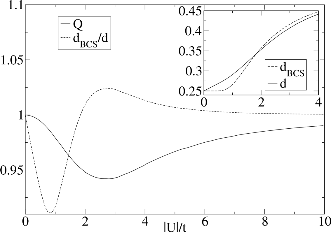
Figure 1: Renormalisation factor $Q$ (solid line) and ratio of double occupancies $d_{\rm BCS}/d$ (dashed line) as a function of $|U|/t$. Inset: double occupancies $d$ (solid line) and $d_{\rm BCS}$ (dashed line).

4.2 Numerical results

As seen in eq. (25) the Gutzwiller–Bogoliubov quasi-particles have a dispersion relation $|E_{k}|=\sqrt{(Q\epsilon_{k}^{0})^{2}+\eta_{\rm s}^{2})}$. The band-width renormalization factor $Q$ in the Gutzwiller theory deviates only slightly from the uncorrelated BCS value $Q=1$, as shown in Fig. 1. It has a minimum $q_{\rm min}\approx 0.95$ for medium-size correlation strength $|U|\approx 3$. In the limit $U\rightarrow-\infty$ the BCS wave function itself has the optimum expectation value $d\approx 1/2$ of double occupancies such that the Gutzwiller correlator $\hat{P}$ cannot achieve any further energy gain. Therefore, the renormalization approaches unity in this limit. In Fig. 1 we also plot the average double occupancy in Gutzwiller and BCS theory (see inset) as well as the ratio of these two quantities. For small values of $|U|$ the double occupancies show a qualitatively different behaviour in both approaches. In Gutzwiller theory we find the well-known linearity $(d-1/4)\sim U$ whereas BCS theory gives the typical exponential dependence, $(d_{\rm BCS}-1/4)\sim\Delta_{0}^{2}\sim\exp[-(1/|U|)]$. The BCS value $d_{\rm BCS}$ is smaller than $d$ only for small values of $|U|$. For larger $|U|$ the limited flexibility of the BCS wave function leads to an overshooting of the double occupancy.

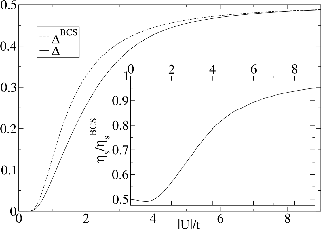
Figure 2: Superconducting order parameters for the Gutzwiller wave function (solid line) and the BCS wave function (dashed line) as a function of $|U|/t$. Inset: Ratio of the superconducting gaps in the Gutzwiller and the BCS theory.

In Fig. 2, we show the values of the superconducting order parameter $\Delta$ in both theories as a function of $U$. The inset of this figure shows the ratio of the two superconducting gaps. Note that in BCS theory we have $\eta^{\rm BCS}_{\rm s}=|U|\Delta^{\rm BCS}$. The order parameters are quite similar in both approaches apart from small values of $|U|$ where

$$\lim_{|U|\rightarrow 0}\frac{\Delta}{\Delta^{\rm BCS}}=\lim_{|U|\rightarrow 0}\frac{\eta_{\rm s}}{\eta_{\rm s}^{\rm BCS}}=r\;.$$ (42)

Other than the order parameter, the superconducting gaps in both theories differ significantly over a large range of correlation parameters $|U|$. Equation (35) shows that BCS theory fails when the density of states at the Fermi energy $D(0)$ becomes small.

5 Summary

As a first application of our recently developed Gutzwiller theory for superconducting systems [10] we investigated the attractive Hubbard model. Our variational approach leads to the diagonalisation of an effective one-particle Hamiltonian, very similar to the corresponding mean-field BCS theory. Quantitatively, however, the resulting quasi-particle band structure differs remarkably from the BCS band energies. This observation holds, in particular, for the superconducting gap in both theories.

In the limit of small Coulomb interaction $|U|/t$, a comparison of our approach with perturbation theory shows that Gutzwiller theory reproduces the renormalization of the superconducting order parameter qualitatively. Quantitatively, the results depend on the bare density of the states of the system. For the semi-elliptic density of states, for example, our renormalization of the gap is too small by a factor of about two.

The condensation energy, i.e., the energy difference between the paramagnetic and the superconducting ground state, is another quantity which is notoriously overestimated in BCS theory. This holds, in particular, for large $U$ where the condensation energy should approach zero but diverges in BCS theory. In contrast, our Gutzwiller theory gives the correct order of magnitude for the condensation energy for all Coulomb strengths.

Apparently, the investigation of superconducting systems with Gutzwiller wave functions leads to a significant improvement over on simple BCS-type calculations. Therefore, our approach should be a useful tool for the investigation of more realistic model systems that exhibit superconductivity.

References

References

• [1] Gutzwiller M C 1963 Phys. Rev. Lett. 10 159
• [2] Hubbard J 1963 Proc. R. Soc. A 276 238
• [3] [] —– 1964 Proc. R. Soc. A 281 401
• [4] Bünemann J 1998 Eur. Phys. J. B 4 29
• [5] Gebhard F 1990 Phys. Rev. B 41 9452
• [6] Gebhard F 1991 Phys. Rev. B 44 992
• [7] Metzner W and Vollhardt D 1988 Phys. Rev. B 37 7382
• [8] Bünemann J, Gebhard F and Weber W 1998 Phys. Rev. B 57 6896
• [9] Bünemann J, Gebhard F, Ohm T, Umstätter R, Weiser S, Weber W, Claessen R, Ehm D, Harasawa A, Kakizaki A, Kimura A, Nicolay G, Shin S and Strocov V N 2003 Eur. Phys. Lett. 61 667
• [10] Bünemann J, Gebhard F and Weber W 2005 Frontiers in Magnetic Materials, ed A Narlikar (Berlin: Springer)
• [11] Zhang F C, Gros C, Rice T M and Shiba H 1988 Supercond Sci. Technol. 1 36
• [12] Gan J Y, Zhang F C and Su Z B 2005 Phys. Rev. B 71 14508
• [13] Anderson P W, Lee P A, Randeria M, Rice T M, Trivedi N and Zhang F C 2004 J. Phys.: Cond. Matt. 16 R755
• [14] Suzuki Y Y, Saito S and Kurihara S 1999 Prog. Theor. Phys. 102 953
• [15] Metzner W 1991 Z. Phys B 82 183
• [16] Bünemann J, Gebhard F and Thul R 2003 Phys. Rev B 67 75103
• [17] van Dongen P G J 1994 Phys. Rev B 50 14016
• [18] Note that the negative-$U$ Hubbard model at half filling and for a bipartite lattice is equivalent to a Hubbard model with positive $U$ (see e.g.: Robaskiewicz S, Micnas and Chao K A 1981 Phys. Rev B 23 1447). Therefore, the superconducting order parameter and the transition temperature can be deduced from the respective antiferromagnetic properties.