Strong disorder renormalization group on fractal lattices:
Heisenberg models and magnetoresistive effects in tight binding models

Abstract

We use a numerical implementation of the strong disorder renormalization group (RG) method to study the low-energy fixed points of random Heisenberg and tight-binding models on different types of fractal lattices. For the Heisenberg model new types of infinite disorder and strong disorder fixed points are found. For the tight-binding model we add an orbital magnetic field and use both diagonal and off-diagonal disorder. For this model besides the gap spectra we study also the fraction of frozen sites, the correlation function, the persistent current and the two-terminal current. The lattices with an even number of sites around each elementary plaquette show a dominant $\phi_{0}=h/e$ periodicity. The lattices with an odd number of sites around each elementary plaquette show a dominant $\phi_{0}/2$ periodicity at vanishing diagonal disorder, with a positive weak localization-like magnetoconductance at infinite disorder fixed points. The magnetoconductance with both diagonal and off-diagonal disorder depends on the symmetry of the distribution of on-site energies.

I Introduction

The interplay between quantum fluctuations, correlations and quenched disorder is a notoriously difficult problem of solid state theory. Recently, however, a strong disorder renormalization group (RG) approach was introduced for a class a low-dimensional random quantum systems, for a review seereview . The idea of this method has been introduced by Ma and DasguptaMaDasgupta and has been widely used after Fisher had shownfisher ; fisherxx that the method provides asymptotically exact results for some one-dimensional problems.

The applicability of the RG method is due to the nature of the low-energy fixed points in these systems. In the so called infinite disorder fixed points at larger scales the disorder grows without limits and therefore completely dominates the low-energy, low-temperature properties of the systems. In an infinite disorder fixed point both dynamical and static singularities are expected, described exactly by the RG method at low energy. The so called strong disorder fixed points, in which the disorder has a limited strength, occur in different systems. At these fixed points only the dynamical singularities are expected to be calculated asymptotically exactly. Infinite disorder fixed points can be found in several 1D systems, for instance in the random transverse field Ising chainfisher , random antiferromagnetic Heisenberg chainfisherxx , tight-binding model, equivalent in 1D to the random XX model by a Jordan-Wigner transformation. Strong disorder fixed points are characterized by Griffiths phasesgriffiths ; igloi99 in the Heisenberg chain with randomly mixed ferro- and antiferromagnetic couplingswesterberg and in random quantum laddersladders .

In higher dimensional systems we have less information about the properties of low-energy fixed points. Models with discrete symmetry, such as the random quantum Ising model, generally have an infinite disorder fixed pointising2D , whereas models with continuous symmetry, such as the random Heisenberg model have a strong disorder fixed pointheis2D . For the random tight-binding model on the square lattice a logarithmically infinite disorder fixed point is conjecturedgade ; huse . Generally, in higher dimensional systems the RG method can be implemented numerically and the analysis of the results is often difficult due to finite size effects.

The core subject of our article is devoted to investigating the properties of the random tight-binding model with diagonal and off-diagonal disorder on fractal lattices through a strong disorder RG. We also make a comparison to random networks of conductors on Euclidean geometries treated by Green’s functions, and to make contact with previous works on spin model, we discuss also the random Heisenberg model on fractal lattices treated by a strong disorder RG. The Heisenberg and tight-binding models have different low-energy fixed points in 1D and in 2D and we want to investigate the properties of this dimensional cross-over using different types of fractal lattices. We use fractals with a sparse structure, so that the RG converges much more rapidly than on the compact higher dimensional Euclidean lattices. Besides the Sierpinski gasket for which we find strong disorder (i.e. not infinite disorder) fixed points, we study a family of quasi-1D lattices that can be cut into two pieces of arbitrary sizes by disconnecting only two bonds, for which we find infinite disorder fixed points. We also investigate the permanent current and the two-terminal conductance. We give a general argument showing that the permanent current is $\phi_{0}/2$-periodic for a tight-binding model with an odd number of sites around each elementary plaquette, with a symmetric diagonal disorder, and with a chemical potential in the middle of the band. We obtain an agreement between this general argument, the permanent current calculated from the RG, and the two-terminal current calculated from the RG and from Green’s functions on Euclidean lattices.

The structure of the paper is the following. The models and the fractals are introduced in Sec.II and the basic ingredients of the strong disorder RG method are presented in Sec.III. Our results are given in Sec.IV and V, for the Heisenberg model and for the tight-binding model, respectively. We close our paper by a Conclusion. Some details are provided in the Appendices.

II Models and lattices

II.1 Random Heisenberg model

The random Heisenberg Hamiltonian is given by

$${\cal H}=\sum_{\langle k,l\rangle}J_{k,l}{\bf S}_{k}.{\bf S}_{l}\;,$$ (1)

where the sum runs over all neighboring pairs of sites, and where ${\bf S}_{k}$ corresponds to a spin-1/2. In the antiferromagnetic model we use $0<J_{k,l}<J_{\rm max}$ and the exchange distribution

$${\cal P}(J)={\cal F}_{\alpha}(J,J_{\rm max})\equiv\alpha\frac{J_{\rm max}^{-\alpha}}{J^{1-\alpha}}\;.$$ (2)

For the Heisenberg model with a symmetric distribution of exchanges we use $-J_{\rm max}<J_{k,l}<J_{\rm max}$. The absolute value of $J$ is distributed according to Eq. (2). The motivation for introducing singular exchange distributions is that the strong disorder RG generates by itself singular renormalized coupling distributions even if we start from the regular distribution with $\alpha=1$.

II.2 Random tight-binding model

The random tight-binding Hamiltonian contains both off-diagonal disorder (terms $t_{k,l}$) and diagonal disorder (terms $\epsilon_{k}$):

$${\cal H}=\sum_{\langle k,l\rangle}\left[t_{k,l}(\phi)c_{l}^{+}c_{k}+t_{l,k}(\phi)c_{k}^{+}c_{l}\right]-\sum_{k}\epsilon_{k}c_{k}^{+}c_{k}\;.$$ (3)

The hopping integrals $t_{k,l}(\phi)$ are complex numbers and depend on the value of the magnetic flux $\phi$ through an elementary plaquette:

$$t_{k,l}(\phi)=t_{k,l}\exp{\left(\frac{2i\pi}{\phi_{0}}\int_{{\bf r}_{k}}^{{\bf r}_{l}}{\bf A}.d{\bf r}\right)},$$ (4)

where the integral over the vector potential is from ${\bf r}_{k}$ to ${\bf r}_{l}$, the two points corresponding to the lattice sites with labels $k$ and $l$. The variables $t_{k,l}$ correspond to the hopping integrals in the absence of a magnetic field.

The on-site energies $\epsilon_{k}$ are chosen in the distribution ${\cal P}(\epsilon)={\cal F}_{\alpha_{\epsilon}}(\epsilon,\epsilon_{\rm max})$, where ${\cal F}$ is given by Eq. (2), and the hopping variables $t_{k,l}$ are chosen in the distribution ${\cal P}(t)={\cal F}_{\alpha_{t}}(t,t_{\rm max})$. To avoid multiplying the number of parameters we restrict to the case $\alpha_{\epsilon}=\alpha_{t}$ and use the notation $\alpha=\alpha_{\epsilon}=\alpha_{t}$.

II.2.1 Correlation functions

The correlation functions of the tight-binding models are defined by

$${\cal C}_{1}(R) = \frac{\lambda}{{\cal N}(R)}\overline{\sum_{\langle k,l\rangle}\langle c^{+}_{k}c_{l}\rangle}$$ (5)

$${\cal C}_{2}(R) = \frac{\lambda}{{\cal N}(R)}\overline{\sum_{\langle k,l\rangle}\langle c^{+}_{k}c_{l}\rangle^{2}},$$ (6)

with the constraint that the distance between sites $k$ and $l$ is equal to $R$. Here and in the following $\langle\dots\rangle$ stands for the thermal average (corresponding to the average in the ground state at $T=0$), and the overline denotes averaging over quenched disorder. ${\cal N}(R)$ is the number of sites at distance $R$ and $\lambda$ is a normalization constant.

We first choose $\lambda$ in such a way that the histograms are normalized to unity:

$$\sum_{R\neq 0}C_{1,2}(R)=1.$$ (7)

The other possibility is to use unnormalized histograms corresponding to $\lambda=1$, that will be noted ${\cal C}_{1,2}^{\prime}(R)$. ${\cal C}_{2}^{\prime}(R)$ will be used for comparing the conductance at different magnetic fields.

II.2.2 Conductance, current and persistent current

The differential conductance ${\cal G}(V,T,R)$ at a fixed temperature $T$, voltage $V$ and distance $R$ is defined as the derivative of the two-terminal current ${\cal I}(V,T)$ with respect to the applied voltage:

$${\cal G}(V,T,R)=\frac{d}{dV}{\cal I}(V,T).$$ (8)

For simplicity we carry out an averaging over all pairs of sites at distance $R$ on the lattice, so that we cannot discuss the geometrical effects related to the position at which an extended contact has been connected to the fractal lattice.

The persistent current $J(\phi,T)$ circulating in the system in the absence of an applied voltage is equal to the derivative of the energy $U(\phi,T)$ with respect to the magnetic flux:

$$J(\phi,T)=-\frac{\partial}{\partial\phi}U(\phi,T).$$ (9)

II.3 The fractal lattices

Figure 1: Representation of the fractal lattices with $n=3$, $g=4$ (a); $n=4$, $g=4$ (b); $n=5$, $g=5$ (c); and the Sierpinski gasket with $g=6$ (d)

We use a family of fractal lattices based on regular polygons with $n$ sides. We denote by $g$ the number of generations. The lattices with $n=3,4,5$ are shown on Fig. 1-(a), (b) and (c). In the case $n=3$ the number of sites $N_{s}$ and the number of links $N_{l}$ is

$$N_{s} = \left[g+\frac{1}{2}\right]3^{g-1}+\frac{3}{2}$$ (10)

$$N_{l} = 3^{g}.$$ (11)

In the case $n>3$ we define $A=(n^{2}-4n+5)/[(n-1)(n-3)]$, $B=-n/[3(n-3)]$, $C=n/(n-1)$, $A^{\prime}=(n-2)/(n-3)$. We have

$$N_{s} = An^{g}+3^{g}B+C$$ (12)

$$N_{l} = A^{\prime}n^{g}+3^{g}B.$$ (13)

The linear length is equal to $3^{g}$ so that the fractal dimension is $d_{f}=\ln{n}/\ln{3}$.

We also use the standard Sierpinski gasket shown on Fig. 1-(d). The number of sites and links are given by

$$N_{s} = 3+\frac{3}{2}\left[3^{g-1}-1\right]$$ (14)

$$N_{l} = 3^{g}.$$ (15)

The linear length is given by $L=2^{g}$ so that the fractal dimension is $d_{f}=\ln{3}/\ln{2}$.

III Strong disorder RG approach

The strong disorder RG approachreview as initiated by Ma and DasguptaMaDasgupta works in the energy space and at each step a term in the Hamiltonian is eliminated to which the largest excitation energy (gap), denoted by $\Omega$, is associated. During this decimation process the energy scale $\Omega$ is lowered, and the number of sites of the lattice $n(\Omega)$, divided by the initial number of sites, is reduced. At the same time new couplings are generated between the remaining sites which were originally connected to the decimated sites.

III.1 RG rules

III.1.1 Heisenberg model

During renormalization the Heisenberg model, if the lattice is more complex than the linear chain, it will transform into a set of spins of different size between them if there are both ferromagnetic and antiferromagnetic couplingsreview . The renormalization rules, as given in the literaturewesterberg ; melin00 ; ladders ; heis2D involve two processes: spin-cluster formation and singlet formation. Two spins $S_{1}$ and $S_{2}$ coupled by a strong exchange $|J_{1,2}|\sim\Omega$ give rise to a spin $S=S_{1}+S_{2}$ if $J_{1,2}<0$ (ferromagnetic coupling) and to a spin $S=|S_{1}-S_{2}|$ if $J_{1,2}>0$ (antiferromagnetic coupling) and $S_{1}\neq S_{2}$. During this spin-cluster formation process the renormalized couplings are calculated by first order perturbation theory. There is singlet formation if $S_{1}=S_{2}$ are coupled antiferromagnetically, in which case the pair of spin $S_{1}$ and $S_{2}$ is eliminated and the renormalized couplings are calculated by second order perturbation theory. The expression of the renormalized couplings can be found in the literaturewesterberg ; melin00 ; ladders ; heis2D .

III.1.2 Tight-binding model

In the case of the tight-binding model there are two transformations. (i) If the largest gap of the system is associated to a diagonal term, say $\epsilon_{k}=\Omega$, a fermion or a hole is frozen at site $k$, and this site is decimated out. We will refer to this process as an $\epsilon$-transformation. (ii) If the largest gap of the system is associated to an off-diagonal term, say $t_{k,l}=\Omega$, a fermion is frozen in a “dimer” made of sites $k$ and $l$ and this dimer is decimated out. We will refer to this process as a $t$-transformation. The RG transformations for a bipartite lattice with $\epsilon_{k}=0$, for all $k$ involves only the $t$-transformation and can be found already in the literaturehuse . A specificity of the non bipartite lattice RG transformations given in Appendix A is that diagonal disorder can be self-generated by the RG, even though diagonal disorder is not present in the initial condition.

III.2 RG flow

During renormalization we monitor the distribution function of the different parameters of the Hamiltonians in Eqs. (1) and (3) as a function of the energy scale $\Omega$. In different systems the distribution of couplings, say $P(J,\Omega)$, might have different characteristics as the fixed point, $\Omega^{*}=0$, is approached.

III.2.1 Infinite disorder fixed point

At the so called infinite disorder fixed points the distributions broadens without limits, so that the ratio of typical renormalized couplings goes to zero or to infinity. In this fixed point it is convenient to introduce the log-energy scale, $\Gamma=-\ln(\Omega_{0}/\Omega)$ (where $\Omega_{0}$ is a reference energy), related to the length-scale, $L\sim n(\Gamma)^{-1/d}$, as

$$\Gamma\sim L^{\psi}\;,$$ (16)

where $n(\Gamma)$ is the density of non-decimated points. The exponent $\psi$ is one of the exponents characterizing the universality class of the infinite disorder fixed point.

This type of fixed point is realized, among others, for the random antiferromagnetic Heisenberg spin chain and for the random tight-binding model in 1D, for which $\psi=1/2$ in the two cases. In an infinite disorder fixed point the distribution of the lowest gap $\Delta$ follows the functional form:

$$P_{L}(\Delta){\rm d}\Delta=L^{-\psi}\tilde{P}\left[\frac{\ln{\Delta}}{L^{\psi}}\right]{\rm d}\ln\Delta\;.$$ (17)

III.2.2 Logarithmically infinite disorder fixed point

At this fixed point the relation between log-energy scale and length-scale is:

$$\Gamma\sim(\ln L)^{\omega+1}\;,$$ (18)

thus the exponent $\psi$ is formally zero. This type of behavior is found in the random tight-binding model on the square lattice. Gadegade found $\omega=1$, whereas Motrunich et al.huse conjectured $\omega=1/2$, see also Ref.mudry . At this fixed point the distribution of the lowest gap is given by:

$$P_{L}(\Delta){\rm d}\Delta=(\ln L)^{\omega+1}\tilde{P}\left[\frac{\ln{\Delta}}{(\ln L)^{-\omega-1}}\right]{\rm d}\ln\Delta\;.$$ (19)

III.2.3 Strong disorder fixed point

At this fixed point the relation between energy scale and length-scale is:

$$\Omega\sim L^{-z}\;.$$ (20)

where $z$ is the disorder induced dynamical exponent. To obtain the true dynamical exponent $z_{0}$ of the system, one should also consider deterministic quantum fluctuations which could results in a vanishing gap and thus a quantum dynamical exponent $z_{q}$. In the non-random system $z_{0}=z_{q}$, whereas in the presence of quenched disorder $z_{0}={\rm max}(z_{q},z)$. Thus, for $z>z_{q}$ the dynamical singularities of the system are determined by disorder effects, otherwise disorder will results in confluent (subdominant) singularities. (In the infinite and logarithmically infinite disorder fixed points $z$ is formally infinite.)

Strong disorder fixed points are found, among others in random antiferromagnetic Heisenberg models on the square and cubic latticesheis2D and generally this behavior is related to quantum Griffiths phasesgriffiths ; igloi99 ; review .

At this fixed point the distribution of the lowest gap is given by:

$$P_{L}(\Delta){\rm d}\Delta=L^{-z}\tilde{P}\left[\frac{\Delta}{L^{z}}\right]{\rm d}\Delta\;.$$ (21)

If the excitations are localized, then for a small, fixed $\Delta$, $P_{L}(\Delta)$ is proportional to the volume, i.e. $P_{L}(\Delta)\sim L^{d}$, from which follows in the limit large $L$ limit:

$$P(\Delta)\sim\Delta^{-1+d/z}\;.$$ (22)

This relation is used in numerical calculations to determine the dynamical exponent. The asymptotic distribution of the gaps at a strong disorder fixed point has a power-law form, that should be compared to the initial distribution in Eq.(2). There are random quantum systems in which $z$ depends on the initial disorder and $z$ is approximately proportional to $1/\alpha$. This can be found, among others for random Heisenberg spin laddersladders . In other systems with frustration, $z$ is disorder independent (see the three-dimensional spin glass modelsheis2D ), and large spins are formed in these cases, as discussed in the following section.

III.2.4 Singlet and large spin formation

In random Heisenberg models during decimation the typical size of the generated new spins can be of two types. i) The renormalized spins are typically $S=1/2$ (or $O(1)$) and do not grow under renormalization. In this case in the ground state typically singlets are formed and we refer to this process as random singlet formation. This type of behavior is found in the 1D random antiferromagnetic Heisenberg modelfisherxx . ii) Another possibility is that during renormalization large spins are formed, the size of which continuously grows during renormalization. The typical size of the effective spin, $S_{eff}$, is asymptotically related to the number of decimated spins, $N$ as:

$$S_{eff}\sim N^{\zeta}\;.$$ (23)

The characteristic exponent $\zeta$ would be $\zeta=1/2$ in an uncorrelated decimation approximationwesterberg ; heis2D . Large spin formation can be found, among others in the $\pm J$ Heisenberg models in one-westerberg , two-heis2D , and three-dimensionsheis2D .

III.3 RG calculation of correlations and transport in the random tight binding model

III.3.1 Correlation functions

During renormalization, as $\Omega$ is gradually decreased, some electrons and holes becomes localized at given sites and do not contribute to the correlation functions in Eq.(5) and (6). There is, however, a complementary process by which electrons are bound on delocalized orbitals connecting remote sites, say $k$ and $l$. Therefore correlations between $k$ and $l$ are $1/2$, if $\tilde{t}_{kl}$ at the decimation energy, $|\tilde{t}_{kl}|=\Omega$, is positive and it is $-1/2$ otherwise. These rare regions dominate the average correlation function. Typical correlations, measured between two sites that are not involved in a delocalized bound state, are much weaker and scale as $\sim\tilde{t}_{kl}/\Omega$. This is indeed negligible if the distribution of $\tilde{t}_{kl}$ is broad. Thus we obtain for the leading behavior of the average correlation function,

$${\cal C}_{1}(\Omega,R)=\frac{\lambda}{2{\cal N}(R)}\sum_{\langle k,l\rangle}s_{kl}\;,$$ (24)

where the sum is over all frozen pairs at distance $R$, and $s_{kl}={\rm sign}(\tilde{t}_{kl})$. We have a similar expression also for ${\cal C}_{2}(\Omega,R)$.

III.3.2 Conductance and current

Here we consider the system with a small applied voltage $V$ and at a small temperature $T$. This will generate an energy scale in the system, $\Omega(V,T)={\max}(eV,T)$, and the renormalization process stops at $\Omega=\Omega(V,T)$. The average value of the differential conductance is dominated by rare regions, in which, at energy scale $\Omega(V,T)$ a frozen extended electron state connects the two electrodes, that are separated by a distance $R$. Since the same rare regions are dominant for the average unnormalized correlation function ${\cal C}_{2}^{\prime}(\Gamma,R)$ we obtain the relation:

$${\cal G}(V,T,R)=\frac{e^{2}}{h}{\cal C}^{\prime}_{2}(\Omega(V,T),R)\;.$$ (25)

A detailed derivation of Eq.(25), based on the perturbative theory of transport processes can be found in Appendix B.

The total current ${\cal I}_{\rm tot}(V,T,R)$ in Eq.(8) is obtained by integrating the differential conductance (25) over voltage, which for a small fixed temperature, $T\ll eV$, is equivalent to an integration over the energy scale, $\Omega$:

$${\cal I}_{\rm tot}(V,T,R)\propto\int_{0}^{\Omega(V,T)}{\cal G}(\Omega^{\prime},R)d\Omega^{\prime}\;.$$ (26)

Eq. (26) constitutes a generalization of the Kubo formula since ${\cal I}_{\rm tot}(V,T,R)$ is not necessarily linear in $V$ in the limit $V\rightarrow 0$. The differential conductance for a large separation between the contacts corresponds to low energies, so that we use the standard form of the RG asymptotically exact in the low energy limit at an infinite disorder fixed point.

III.3.3 Persistent current

The zero temperature persistent current in Eq.(9) is related to the average energy

$$U(\phi,T)=\int_{\Omega(T)}^{\Omega_{0}}\left[-\Omega p_{t}(\Omega)-\frac{\Omega}{2}p_{\epsilon}(\Omega)\right],$$ (27)

where $p_{t}(\Omega)$ and $p_{\epsilon}(\Omega)$ are the probabilities to perform respectively a $t$- or and $\epsilon$-transformation at energy scale $\Omega$. We have subtracted in Eq. (27) the energy $U(\phi,+\infty)$ at infinite temperature. The infinite temperature energy in a $t$ transformation is vanishingly small since the spectrum of a dimer is symmetric. The infinite temperature energy in an $\epsilon$-transformation is equal to $\epsilon/2$. The $\epsilon$ state is occupied only below the Fermi level, leading to the energy $\epsilon\theta(-\epsilon)$ (with $\theta(\epsilon)=1$ if $\epsilon>0$ and $\theta(\epsilon)=0$ if $\epsilon<0$). Subtracting $\epsilon/2$ yields $-|\epsilon|/2$, leading to Eq. (27).

IV Random Heisenberg models

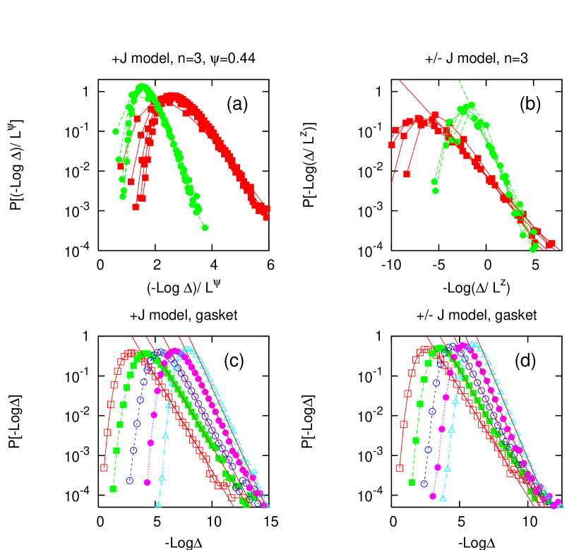
Figure 2: (a) Collapse plot of the gap spectra for the antiferromagnetic Heisenberg model on the fractal with $n=3$. (b) Collapse plot of the gap spectra for the Heisenberg model with a symmetric distribution of exchanges (noted $\pm J$ models on the figure) on the fractal with $n=3$. We use $\alpha=0.25$ ($\Box$, red) and $\alpha=0.5$ ($\bullet$, green) on (a) and (b) respectively. We collapsed the gap spectra with $g=3,4,5,6,7$ generations. (a) corresponds to the scaling (17) with $\psi=0.44$ while (b) corresponds to the conventional disorder scaling given by Eq. (21). The corresponding values of $z$ are shown in Fig. 3. The gap spectra of the antiferromagnetic Heisenberg model and of the Heisenberg model with a symmetric distribution of exchanges are shown on (c) and (d) for $g=3$ ($\blacksquare$, red), $g=4$ ($\Box$, green), $g=5$ ($\circ$, blue), $g=6$ ($\bullet$, purple), and $g=7$ ($\triangle$, blue).

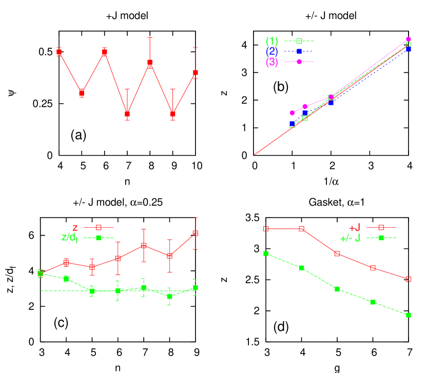
Figure 3: (a) $\psi$ versus $n$ for the antiferromagnetic Heisenberg model. (b) $z$ versus $1/\alpha$ (proportional to the strength of disorder) for the Heisenberg model with a symmetric distribution of exchanges (noted $\pm J$ model on the figure). The curve (1) ($\Box$, green) corresponds to $n=3$ and $n=5$ with $z$ determined from the scaling form (21) of the gap spectra (the points for $n=3$ and $n=5$ are superimposed). The error-bars are comparable to the size of the symbols. The curves (2) ($\blacksquare$, blue) and (3) ($\bullet$, purple) correspond to $n=3$ and $n=5$ respectively, with $z$ determined from the slope of the rare event tail of the gap spectra. (c) Variations of $z$ ($\Box$, red) and $z/d_{f}$ ($\blacksquare$, green) versus $n$ for Heisenberg model with a symmetric distribution of exchanges with $\alpha=0.25$. (d) Variation of $z$ (determined from the slope of the rare event tail of the gap spectra) versus $g$ for the antiferromagnetic Heisenberg model ($\Box$, red) and the Heisenberg model with a symmetric distribution of exchanges ($\blacksquare$, green) on the gasket with $\alpha=1$.

To make contact with previous works on localized spin models in 1D, 2D and 3D we first consider the Heisenberg model on fractal lattices before investigating the tight-binding models on the same lattices. In the numerical calculations we considered random Heisenberg models on the family of fractals with $n=3,...10$ and on the gasket, for a purely antiferromagnetic exchange distribution and for the symmetric exchange distribution with mixed ferromagnetic and antiferromagnetic couplings. The strong disorder RG procedure is implemented numerically and the decimation is performed either up to the last remaining (large) spin or up to the last singlet and the corresponding gap, $\Delta$, is calculated. From the distribution of the gap $P(\Delta)$, the properties of the fixed point are determined using the results overviewed in Sec.III.2. The number of generations is $g=3,4,5,6,7$ for $n=3$, $g=3,4,5,6$ for $n=4$, $g=3,4,5$ for $n=5,6$, $g=3,4$ for $n=7,8,9,10$. We use $\alpha=0.25,0.5,0.75,1$ for $n=3,4$, and $\alpha=0.25$ for $n=5,6,7$. We use $250000$ realizations of disorder in each simulation.

IV.1 Distribution of the gap

IV.1.1 Known results on regular lattices

In 1D the random antiferromagnetic Heisenberg modelfisherxx has an infinite disorder fixed point with the exponent $\psi=1/2$. On the contrary the $\pm J$ model in 1D has a strong disorder fixed pointwesterberg with a finite dynamical exponent, $z=2.3$ and a large-spin with $\zeta=1/2$. Quasi-one-dimensional models, i.e. spin ladders with random antiferromagnetic couplings have a strong disorder fixed point in which the dynamical exponent is approximately proportional to the strength of disorder, i.e. to $\alpha^{-1}$ starting with the distribution in Eq.(2)ladders .

In 2D the random antiferromagnetic model on the square lattice, which is non-frustrated, has a strong disorder fixed point, in which the dynamical exponent is approximately constant for weak disorderheis2D , but for stronger disorder $z$ becomes disorder dependentbilayer . On the other hand for frustrated models (of geometric origin or for the $\pm J$ model) there is a strong disorder fixed point with a large spin. This fixed point with $z=d$ and $\zeta=1/2$ is disorder independent and was called a “spin glass” fixed pointheis2D . There are less accurate numerical results in 3D, but it is likely that a similar scenario as in 2D holds also in 3Dheis2D .

IV.1.2 Random antiferromagnetic model

The results shown in Figs. 2 and 3 suggest that for the antiferromagnetic Heisenberg model the fractals with $n$ even correspond to a infinite disorder fixed point described by the usual scaling with $\psi=1/2$ whereas the fractals with $n$ odd correspond to non trivial infinite disorder fixed points with $\psi$ lower than $1/2$ (see Fig. 3-(a)). The ground state is always a singlet for $n$ even whereas there is large spin formation for $n$ odd. An inspection of the RG flow indicates that spins $1$ and higher are generated in the RG for $n$ even but correspond to an irrelevant perturbation since they disappear soon after they are formed. The uncertainty in the determination of $\psi$ for $n=7,8,9,10$ on Fig. 3 is due to finite size effects since we cannot simulate large values of $g$ for these values of $n$. The error-bar is estimated from the finite size effects with $n=4$.

IV.1.3 Random $\pm J$ model

The gap spectra of the Heisenberg model with a symmetric distribution of exchanges are well described by the strong disorder scaling (21), for both $n$ even and $n$ odd. The value of $z$ can be extracted either from the collapse of the gap spectra given by Eq. (21) or from Eq.(22) by fitting the rare event tail. We have performed both analysis and obtained - within the error of the calculation - identical results. The disorder induced dynamical exponent is found proportional to the initial strength of disorder $1/\alpha$, and we obtained approximately: $z\simeq 0.3d_{f}/\alpha$. This corresponds to the green dashed line in Fig. 3-(c) for $\alpha=0.25$.

IV.1.4 Results on the Sierpinski gasket

For the Sierpinski gasket we find that disorder at the end of the RG decreases as the system size increases, both for the antiferromagnetic Heisenberg model and the Heisenberg model with a symmetric distribution of exchanges (see Fig. 3-(d)). The effective, size dependent dynamical exponent seems to tend to zero as $1/\ln N$. This implies that either i) there is a small finite gap in the system or ii) although the gap is vanishing the dynamical correlations decay faster than a power-law. However, due to the limited sizes of the systems we cannot further study these scenarios.

IV.2 Distribution of the spin of the ground state

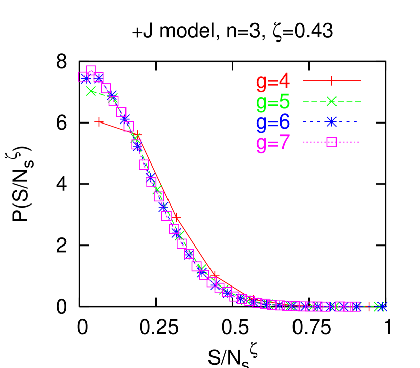
Figure 4: Collapse plot of the distribution of the spin in the ground state for the Heisenberg model on the fractal with $n=3$, for $g=4,5,6,7$ and $\zeta=0.43$. The collapse plot corresponds to Eq. (23).

There is large spin formation for the antiferromagnetic Heisenberg model on the fractal with $n$ odd, and for the Heisenberg model with a symmetric distribution of exchanges for all values of $n$. In all cases we find that the scaling in Eq. (23) is well obeyed. We find for the exponent $\zeta=0.43\pm 0.02$ for the antiferromagnetic Heisenberg model with $n=3$ (see Fig. 4) and $\zeta=0.5$ in all other cases.

IV.3 Conclusion

Table 1: Low-energy fixed points of random Heisenberg models on fractals. For a comparison results on regular 1D and 2D (square) lattices are also presented. (AF: antiferromagnetic couplings, $\pm J$: mixed antiferromagnetic and ferromagnetic couplings, ID: infinite disorder fixed point, SD: strong disorder fixed point, RS: random singlet formation, LS: large spin formation.) ⁽⁺⁾ For $n=3$, $\zeta<1/2$.

	$n=odd$	$n=even$	gasket	1D	2D
AF	ID($\psi=1/2$)	ID($\psi<1/2)$	SD($z\to 0$)(?)	ID($\psi=1/2$)	SD
	LS($\zeta=1/2^{(+)}$)	RS	LS($\zeta=1/2$)	RS	RS
$\pm J$	SD($z\sim 1/\alpha$)	SD($z\sim 1/\alpha$)	SD($z\to 0)$(?)	SD($z=2.3$)	SD($z=d$)
	LS($\zeta=1/2$)	LS($\zeta=1/2$)	LS($\zeta=1/2$)	LS($\zeta=1/2$)	LS($\zeta=1/2$)

The empirically obtained critical behavior of the random Heisenberg model on different fractal lattices is summarized in Table 1. The low-energy fixed point seems to depend on the form (symmetry) of disorder, the symmetry of the fractal lattice, but there is no direct relation to the fractal dimension of the lattice. Interestingly the studied fractal lattices constitute low-energy universality classes that can not be found in the regular 1D and 2D lattices.

V Random tight-binding models

The detail of the RG transformations of the tight-binding model can be found in Appendix A. The interferences between different trajectories in the $t$-transformation are eliminated if the sum of the different terms in the renormalized coupling is replaced by their maximum, an approximation used in the study of spin models. To keep interferences, we do not use the maximum in the expression of the renormalized couplings.

V.1 Features of the RG flow without extrinsic diagonal disorder

V.1.1 Fraction of frozen sites

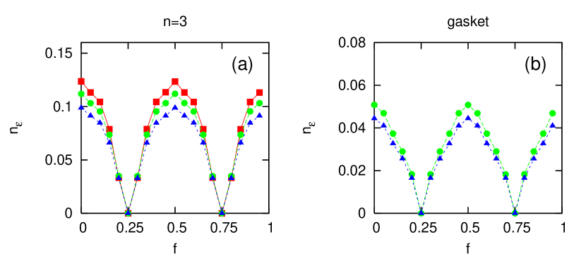
Figure 5: Fraction of frozen sites $n_{\epsilon}$ (defined by Eq. (28)) versus $f$ (a) for the fractal with $n=3$ and $g=4$ ($\blacksquare$, red), $g=5$ ($\bullet$, green) and $g=6$ ($\blacktriangle$, blue); and (b) for the gasket with with $g=4$ ($\blacksquare$, red), $g=5$ ($\bullet$, green) and $g=6$ ($\blacktriangle$, blue) generations. We used $\alpha=1$.

We first consider the case where diagonal disorder is not introduced in the initial condition. We thus start with $\epsilon_{k}=0$ for all $k$. For a bipartite lattice (for instance the fractal with $n$ even) no diagonal term is generated during the RG transformations, which can be seen from the decimation rules given in Appendix A. On the contrary for a non bipartite lattice (for instance for the fractal with $n$ odd) also non vanishing values of $\epsilon_{k}$ are generated, and at the end of the RG an average number $N_{\epsilon}$ of the total number of sites $N_{s}$ has been frozen by the $\epsilon$-transformations. We have calculated the fraction of frozen fermions,

$$n_{\epsilon}=N_{\epsilon}/N_{s}$$ (28)

for both the fractal with $n=3$ and for the gasket. We work in the grand canonical ensemble where the chemical potential is fixed.

We show in Fig. 5 the variation of $n_{\epsilon}$ as a function of $f=\phi/\phi_{0}$. First we note that $n_{\epsilon}$ decreases slowly with increasing system size: in the limit $N_{s}\rightarrow\infty$ our data indicate an approximately logarithmic dependence, $n_{\epsilon}\sim 1/\ln{N_{s}}$. In a finite size system $n_{\epsilon}$ shows $\phi_{0}/2$-oscillations so that the number of frozen fermions vanishes at $f=0.25,0.75,1.25,...$ and there is a tendency of the system to be more localized for $f=0,1/2,1...$, in agreement with the positive magnetoconductance discussed later in section V.5. The cancellation of $n_{\epsilon}$ for $f=0.25,0.75,1.25,...$ can be understood from the renormalization of $\epsilon$ in the $t$-transformation (see Eq. 41). If the sites “1” and “2” are eliminated in a three-site cluster $\{1,2,3\}$ then the interference of the trajectories $3\rightarrow 1\rightarrow 2\rightarrow 3$ and the trajectory $3\rightarrow 2\rightarrow 1\rightarrow 3$ are such that $\tilde{\epsilon}_{3}=0$, so that no diagonal disorder is generated by the RG for these values of $f=\phi/\phi_{0}$.

V.1.2 Average coordinance

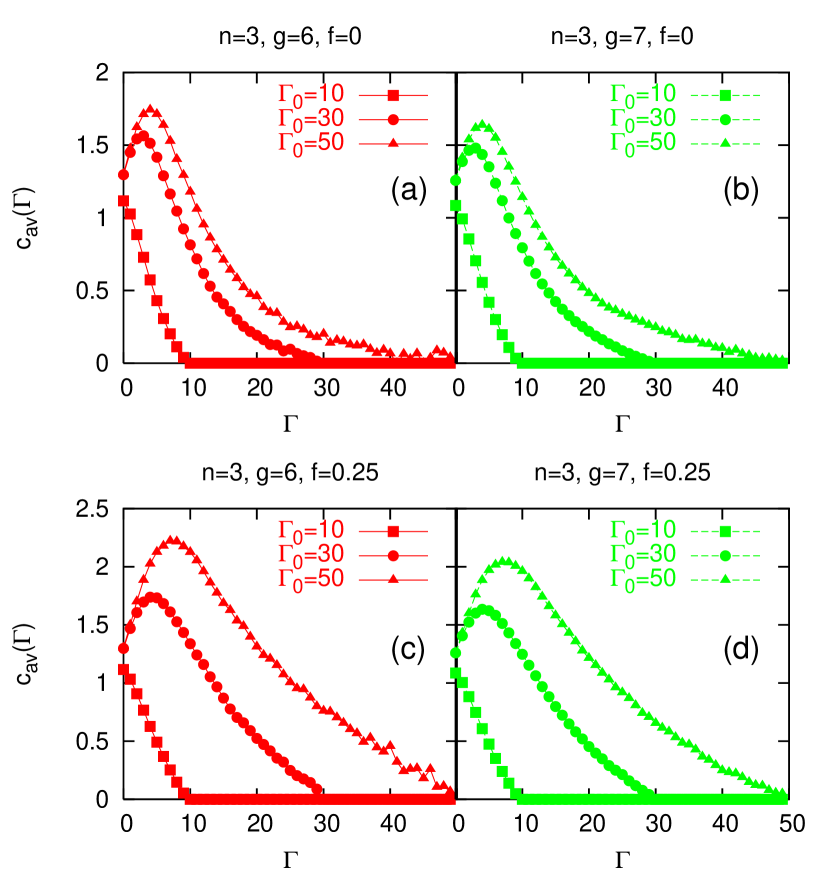
Figure 6: Average coordinance of the graph of “active” spins as a function of $\Gamma$, for different values of $\Gamma_{0}$, for the fractal with $n=3$. (a) corresponds to $g=6$ generations and $f=0$. (b) corresponds to $g=7$ and $f=0$. (c) corresponds to $g=6$ and $f=0.25$. (d) corresponds to $g=7$ and $f=0.25$. The different curves in each panel correspond to $\Gamma_{0}=10$ ($\blacksquare$), $\Gamma_{0}=30$ ($\bullet$) and $\Gamma_{0}=50$ ($\blacktriangle$). The red color is used for $g=6$ and the green color for $g=7$. We used $\alpha=0.25$.

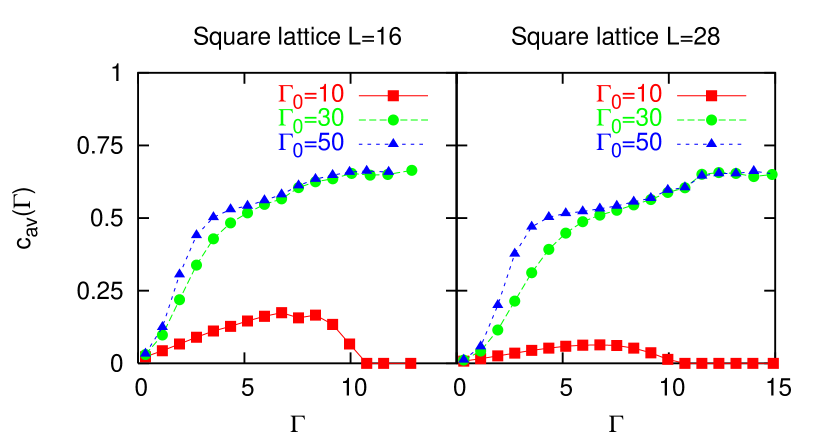
Figure 7: Variation of the average clustering coefficient $c^{\prime}_{\rm av}(\Gamma)$, see text, as a function of $\Gamma$, for different values of $\Gamma_{0}$, for the Euclidian 2D square lattice with $f=0$. (a) corresponds to $L=16$ and (b) corresponds to $L=28$. The different curves in each panel correspond to $\Gamma_{0}=10$ ($\blacksquare$, red), $\Gamma_{0}=30$ ($\bullet$, green) and $\Gamma_{0}=50$ ($\blacktriangle$, blue). We used $\alpha=0.25$.

A useful information is encoded in the connectivity of the graph of “active” sites (the sites that have not been eliminated at the energy scale $\Omega$). More precisely we consider the connectivity of clusters of “strongly connected” sites, which are defined by having hopping amplitudes $t_{k,l}$ that exceed a limiting value:

$$\ln{\left[\frac{\Omega}{|t_{k,l}|}\right]}<\Gamma_{0},$$ (29)

where $\Gamma_{0}$ is a given cut-off.

We calculate the average coordinance $c_{\rm av}$ of this graph as a function of the log-energy scale $\Gamma$, where $c_{\rm av}$ is defined as the ratio of the average number of bonds and the average number of sites. The average coordinance $c_{\rm av}$ is expected to start from a value of order unity, first increase, reach a maximum, and then decrease to zero at large $\Gamma$ since only a few sites are surviving at the end of the RG.

$c_{\rm av}(\Gamma)$ is shown in Fig. 6 for the fractal with $n=3$, for two sizes corresponding to $g=6,7$, and for $f=0$ and $f=0.25$. It is visible that there are practically no finite size effects for $g=6,7$. The average coordinance is larger for $f=0.25$ than for $f=0$, compatible with the existence of a negative magnetoresistance discussed in section V.5: the system is more connected and therefore more delocalized for $f=0.25$.

By comparison we carried out a similar simulation for the Euclidian two-dimensional square lattice. The finite size effects indicate that after a transient the graph of surviving sites becomes extremely connected whereas it is loosely connected in the case of the fractal with $n=3$. This geometrical effect is related to the fact that the algorithm becomes extremely slow in the case of the Euclidian square lattice as compared to the fractal lattices. More quantitatively it is convenient to evaluate the clustering coefficient $c^{\prime}_{\rm av}(\Gamma)$, which is the average fraction of bonds, relative to the maximum number of possible bonds, $N_{s}(N_{s}-1)/2$. For sufficiently large values of $\Gamma_{0}$ the quantity $c^{\prime}_{\rm av}(\Gamma)$ reaches a plateau at around $0.7$, see Fig.7, indicating that the graph of active sites becomes strongly connected.

V.1.3 Gap spectra

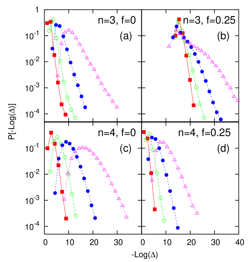
Figure 8: Gap spectra of the tight binding model with ($n=3$, $f=0$) (a), ($n=3$, $f=0.25$) (b), ($n=4$, $f=0$) (c), and ($n=4$, $f=0.25$) (d). The simulations on (a) and (b) with $n=3$ correspond to for $g=4$ ($\blacksquare$, red), $g=5$ ($\circ$, green) $g=6$ ($\bullet$, blue), and $g=7$ ($\triangle$, purple). The simulations on (c) and (d) with $n=4$ correspond to $g=3$ ($\blacksquare$, red), $g=4$ ($\circ$, green), $g=5$ ($\bullet$, blue), and $g=6$ ($\triangle$, purple). We used $\alpha=1$.

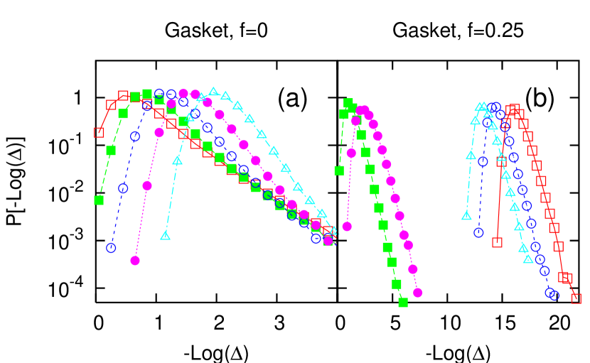
Figure 9: Gap spectra of the tight binding model on the Sierpinski gasket with $f=0$ (a) and $f=0.25$ (b) and with $g=3$ (red, $\square$), $g=4$ (green, $\blacksquare$), $g=5$ (blue, $\circ$), $g=6$ (purple, $\bullet$) and $g=7$ (blue, $\triangle$) generations. We used $\alpha=1$.

We show in Fig. 8 for the fractals with $n=3,4$ the gap spectra of the random tight-binding model with $\epsilon_{\rm max}=0$ and $f=0,0.25$. In all these cases there is infinite disorder scalingnote1 , see Sec.III.2.1. The collapse plots according to Eq. (17) show that $\psi=0.54\pm 0.04$ for ($f=0$, $n=3$), $\psi=0.5\pm 0.03$ for ($f=0$, $n=4$), $\psi=0.48\pm 0.02$ for ($f=0.25$, $n=4$). To obtain the scaling for ($f=0.25$, $n=3$) we repeated the simulations in Fig. 8-(b) without the last $\epsilon$-transformation and found that the scaling is well described by $\psi=0.48\pm 0.02$.

The gap spectra for the gasket shown in Fig. 9 indicate strong disorder scaling, see Sec.III.2.3. The parity effect for $f=0.25$ is similar to the fractal with $n=3$ and $f=0.25$ in Fig. 8, seenote1 . For the Sierpinski gasket the number of sites $N_{s}$ is odd for $g$ odd and even for $g$ even.

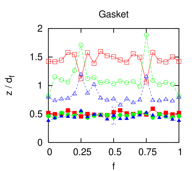
Figure 10: Ratio $z/d_{f}$ versus $f$ for the Sierpinski gasket with ($g=4$, $\alpha=1$) ($\blacksquare$, red), ($g=5$, $\alpha=1$) ($\bullet$, green) and ($g=6$, $\alpha=1$) ($\blacktriangle$, blue), ($g=4$,$\alpha=0.25$) ($\square$, red), ($g=5$,$\alpha=0.25$) ($\circ$, green) and ($g=6$, $\alpha=0.25$) ($\triangle$, blue). The ratio $z/d_{f}$ is smaller than unity for sufficiently large system sizes.

We show in Fig. 10 the variation of the ratio $z/d_{f}$ versus $f$ for the Sierpinski gasket, as calculated from Eq. (22). For a weaker initial disorder ($\alpha=1$) the dynamical exponent is practically independent of $f$ and has no finite size effect, so we can estimate $z/d_{f}=0.5$. The finite size effects are also stronger for stronger initial disorder ($\alpha=0.25$). The dynamical exponent for very large system sizes is probably $f$-independent, and the apparent variations are within the accuracy of the numerical calculation. From the available data it is difficult to estimate the limiting value. However, $z/d_{f}$ (the strength of disorder at the fixed point) increases with $1/\alpha$ (the strength of disorder in the initial condition), so that we might assume that the limiting value of $z/d_{f}$ could be close to $0.5$ for $\alpha=0.25$.

V.2 Normalized correlation functions

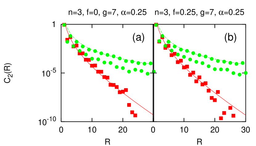
Figure 11: Normalized correlation function ${\cal C}_{2}(\Gamma,R)$ versus $R$ for the fractal with $n=3$ with $g=7$ generations, ${\alpha=0.25}$ and $f=0$ (a), $f=0.25$ (b). The different curves correspond to $\Gamma=5$ ($\blacksquare$, red), $\Gamma=30$ ($\bullet$, green). The solid lines correspond to the fit (30), with $x=1.6$ and $\xi(\Gamma)=2.5$ for $\Gamma=5$, and $\xi(\Gamma)=+\infty$ for $\Gamma=30$.

The definition of the correlation function is given in section III.3.1. The correlation functions obtained from the simulations are well fitted by

$${\cal C}_{2}(\Gamma,R)\sim\frac{1}{R^{2x}}\exp{\left(-\frac{R}{\xi(\Gamma)}\right)},$$ (30)

with a correlation length $\xi(\Gamma)$ diverging like $\xi(\Gamma)\sim\Gamma^{1/\psi}$ at an infinite disorder fixed point, see Eq.(16). For the Euclidean 1D random tight-binding model we have $x=1$ from the simulation, in agreement with the analytical predictionfisherxx . For the fractals with $n=3$ and $n=4$, we obtain the same values of the decay exponent $x$ and the correlation length $\xi(\Gamma)$, for ${\cal C}_{1}(\Gamma,R)$ and ${\cal C}_{2}(\Gamma,R)$. This is expected since the dominant contribution to the correlation functions is due to the same type of rare regions for both functions. The decay length of ${\cal C}_{1}(\Gamma,R)$ is equal to the decay length of ${\cal C}_{2}(\Gamma,R)$, a feature of 1D Euclidean systems that we recover on the sparse fractal lattices. In usual disordered systems with diagonal disorder and no off-diagonal disorder, the decay length of ${\cal C}_{1}(R)$ at zero temperature is equal to the elastic mean free path, and the decay length of ${\cal C}_{2}(R)$ at zero temperature is equal to the localization length. At finite temperature there exists an additional exponential decay over the thermal length $\xi_{T}$. The situation considered here with off-diagonal disorder and diagonal disorder can be viewed as a temperature dependent mean free path equal to the temperature dependent localization length. Like in 1D systems, there is no genuine diffusive regime in which the localization length would be much larger than the elastic mean free path. Interestingly, we still obtain a weak localization-like magnetoresistance for the fractal with $n=3$ (see Secs.V.4 and V.5).

The variation and the fit of ${\cal C}_{2}(\Gamma,R)$ versus $R$ is shown in Fig. 11 for the fractal with $n=3$. We used $x=1.6$ for all values of $\alpha$ but, as expected, $\xi(\Gamma)$ increases as $\alpha$ increases (not shown in Fig. 11). The same value of $x$ is obtained for $n=4$ (not shown in Fig. 11). We find no significative difference in the values of $x$ and $\xi(\Gamma)$ between the cases $f=0$ and $f=0.25$.

There exists a parity effect like in 1D. Namely the correlations between two sites at distance $R$ are much stronger if $R$ is odd. The origin of this effect in $1D$ is that all the sites in between should be coupled in localized pairs in order to have an extended localized orbital between the two remote sites at distance $R$. This is obviously only possible for $R$ odd. Similar effect might be due to the $1D$ chains embedded in the fractal with $n=3$.

V.3 Effect of extrinsic diagonal disorder at $f=0$

V.3.1 Fraction of frozen sites

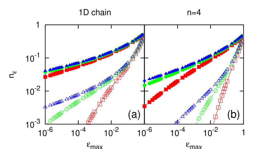
Figure 12: Variation of the fraction of sites $n_{\epsilon}$ frozen by an $\epsilon$-transformation as a function of $\epsilon_{\rm max}$, the upper cut-off in the distribution of $\epsilon$, for the 1D chain (a) and the fractal with $n=4$ (b). For the 1D chain on (a) we used chains of length $L=100$ ($\blacksquare$ and $\square$, red), $L=400$ ($\bullet$ and $\circ$, green) and $L=1600$ ($\blacktriangle$ and $\triangle$, blue). For the fractal with $n=4$ on (b) we used $g=3$ ($\blacksquare$ and $\square$, red), $g=4$ ($\bullet$ and $\circ$, green) and $g=5$ ($\blacktriangle$ and $\triangle$, blue). The open symbols correspond to $\alpha=1$ and the filled symbols correspond to $\alpha=0.25$.

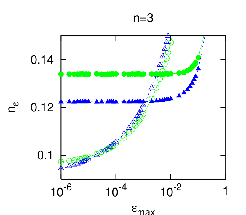
Figure 13: Variation of the fraction of sites $n_{\epsilon}$ frozen by an $\epsilon$-transformation as a function of $\epsilon_{\rm max}$, the upper cut-off in the distribution of $\epsilon$, for the fractal with $n=3$. We used $g=4$ ($\bullet$ and $\circ$, green) and $g=5$ ($\blacktriangle$ and $\triangle$, blue). The open symbols correspond to $\alpha=1$ and the filled symbols correspond to $\alpha=0.25$. We obtained a similar behavior for $n=5$.

We now consider the case of a finite extrinsic diagonal disorder with $f=0$. Increasing $\epsilon_{\rm max}$ tends to increase the number of $\epsilon$-transformation and thus the fraction of frozen sites $n_{\epsilon}(\epsilon_{\rm max})$. For bipartite lattices, such as the 1D chain and the fractal with $n=3$ the limiting value of $n_{\epsilon}(\epsilon_{\rm max})$ is finite in the limit $\epsilon_{\rm max}\to 0$, even for a finite lattice. This behavior is illustrated in Fig. 12. The limiting behavior of $n_{\epsilon}(\epsilon_{\rm max})$ can be estimated as follows. For a small fixed $\epsilon_{\rm max}$, the RG transformation goes along the trajectory of the $\epsilon_{\rm max}=0$ case, until the log-energy scale $\Gamma=\ln(\epsilon_{0}/\epsilon_{\rm max})$ is reached, with some reference value $\epsilon_{0}$. At this point $n_{\epsilon}(\epsilon_{\rm max},N_{s})$ is proportional to the number of sites $N_{s}$. The infinite disorder scaling given by Eq. (16) corresponds to $\ln(\epsilon_{0}/\epsilon_{\rm max})\sim\Gamma\sim N_{s}^{\psi/d_{f}}$. We thus obtain a logarithmic dependence as $n_{\epsilon}(\epsilon_{\rm max})\sim(\ln(\epsilon_{0}/\epsilon_{\rm max}))^{d_{f}/\psi}$. The numerical data in Fig. 12 are compatible with this form, although a simple power-law form $n_{\epsilon}(\epsilon_{\rm max})\sim\epsilon_{\rm max}^{y}$, with an effective exponent $y=0.14$ seems to work, too, both for the 1D chain and the fractal with $n=4$.

For a non-bipartite lattice, such as the fractal with $n=3$, $n_{\epsilon}$ tends to a constant in the limit $\epsilon_{\rm max}\rightarrow 0$ for a finite lattice, see Sec.V.1.1. This is illustrated in Fig. 13. For a small $\epsilon_{\rm max}$, $n_{\epsilon}$ increases as the system size increases for bipartite (the 1D and the fractal with $n=4$) lattices and decreases for non-bipartite (the fractal with $n=3$) lattices.

V.3.2 Correlation length

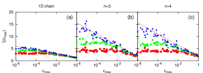
Figure 14: Average correlation length $\xi_{av}(\Gamma,\epsilon_{\rm max})$ as a function of $\epsilon_{\rm max}$ for several values of $\Gamma$, for the 1D chain (a), the fractal with $n=3$ (b) and the fractal with $n=4$ (c). In (a) we use $\Gamma=7$ ($\blacksquare$, red), $\Gamma=9$ ($\bullet$, green), $\Gamma=11$ ($\blacktriangle$, blue). In (b) and (c) we use $\Gamma=5$ ($\blacksquare$, red), $\Gamma=8$ ($\bullet$, green), $\Gamma=11$ ($\blacktriangle$, blue), We use $\alpha=0.25$, $L=6400$ for the 1D chain, $g=7$ for the fractal with $n=3$, and $g=6$ for the fractal with $n=4$. The fits correspond to $\xi_{\rm av}(\Gamma,\epsilon_{\rm max})=a\ln{(\epsilon_{\rm max}/\Omega_{0})}+b$, with $a=0.35$ and $b=1.2$ for the 1D chain, and $a=1$ and $b=1.8$ for the fractals with $n=3$ and $n=4$. We obtained qualitatively similar results for other values of $\alpha$, and for the “$\pm\epsilon$” model with a symmetric distribution of $\epsilon$.

The average correlation length $\xi_{av}(\Gamma,\epsilon_{\rm max})$ is calculated from the average correlation function ${\cal C}_{2}(\Gamma,R)$. Using the functional form in Eq. (30) we fix the decay exponent $x$ to its value for $\epsilon_{\rm max}=0$ (see Sec. V.2), and then extract the value of $\xi_{av}(\Gamma,\epsilon_{\rm max})$ from the numerical data. The numerical results are shown in Fig.14 for the 1D chain (a) and for the fractals with $n=3$ (b) and $n=4$ (c). In the limit $\Gamma\gg\ln(\epsilon_{\rm max}/\epsilon_{0})$ the average correlation length has a $\Gamma$ independent limiting value which depends on $\ln(\epsilon_{\rm max}/\epsilon_{0})$ and the functional form seems to be linear for all type of lattices. Here we can observe an analogy with the behavior of the average correlation length in a disordered Heisenberg chain used as a model of disordered spin-Peierls system at a finite temperature $T$, as calculated in Ref.FM-PRB . Making the correspondence with the energy scales in the two problems, $\epsilon_{\rm max}\leftrightarrow T$, we arrive to the relation $\xi_{av}(\Gamma,\epsilon_{\rm max})\sim\ln(\epsilon_{\rm max}/\epsilon_{0})$ for $\Gamma\gg\ln(\epsilon_{\rm max}/\epsilon_{0})$, as observed numerically.

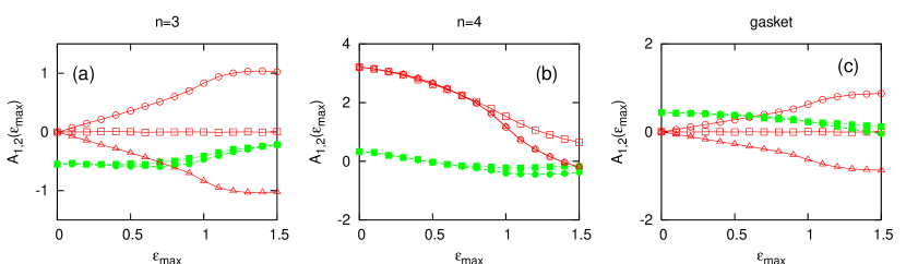
Figure 15: Evolution of the harmonics $A_{1}(\epsilon_{\rm max})$ (open symbols,red) and $A_{2}(\epsilon_{\rm max})$ (filled symbols, green) of the permanent current, as a function of $\epsilon_{\rm max}$. Panel (a), (b) and (c) correspond respectively to the fractals with $n=3$, $n=4$ and to the Sierpinski gasket. The different curves within each panel correspond to the “$\pm\epsilon$” model with a symmetric distribution of $\epsilon_{k}$ ($\Box$ and $\blacksquare$), to the “$+\epsilon$” model with $\epsilon_{k}>0$ ($\circ$ and $\bullet$), and to the “$-\epsilon$” model with $\epsilon_{k}<0$ ($\triangle$ and $\blacktriangle$).

V.4 Persistent current

V.4.1 General argument

We expect the averaged persistent current to exhibit a $\phi_{0}/2$ periodicity for any tight-binding lattice with an odd number of sites around its elementary plaquettes, provided the distribution of diagonal disorder is even and the chemical potential $\mu$ is fixed equal to zero. The following argument is inspired by the discussion given inBrowne84 for Aharonov-Bohm current oscillations in a mesoscopic ring. The eigenvalue equation for the single-particle Hamiltonian (3) reads:

$$E\psi_{k}=-\epsilon_{k}\psi_{k}+\sum_{l}t_{kl}(\phi)\psi_{l}$$ (31)

If we multiply this equation by $-1$, we get an eigenstate with energy $-E$, for a tight-binding model where on-site potentials and hopping amplitudes have been turned into their opposite values. On a bipartite lattice, changing $t_{kl}(\phi)$ into $-t_{kl}(\phi)$ is simply equivalent to performing a gauge transformation, which leaves the external magnetic field unchanged. But on a lattice (such as a triangular lattice) with elementary odd cycles, this change of sign in the hopping amplitudes is equivalent to changing the elementary flux $\phi$ into $\phi+\phi_{0}/2$. Denoting single-particle energy eigenvalues by $E_{\alpha}(\phi,\{\epsilon_{k}\})$, we have then

$$\sum_{\alpha}E_{\alpha}(\phi,\{\epsilon_{k}\})\theta(\mu-E_{\alpha})$$ (32)

$$+ \sum_{\beta}E_{\beta}(\phi+\frac{\phi_{0}}{2},\{-\epsilon_{k}\})\theta(E_{\beta}+\mu)=0$$ (33)

Let us then average these expressions over disorder realizations. Since the $\epsilon_{k}$ distribution is assumed to be even, this yields:

$$\sum_{\alpha}\overline{E_{\alpha}(\phi)\theta(\mu-E_{\alpha})}+\sum_{\beta}\overline{E_{\beta}(\phi+\frac{\phi_{0}}{2})\theta(E_{\beta}+\mu)}=0$$ (34)

The sum-rule on the single-particle spectrum yields

$$\sum_{\beta}\overline{E_{\beta}(\phi+\frac{\phi_{0}}{2})(\theta(E_{\beta}+\mu)+\theta(-\mu-E_{\beta}))}$$ (35)

$$= -\sum_{k}\overline{\epsilon_{k}}=0$$

So finally:

$$\sum_{\alpha}\overline{E_{\alpha}(\phi)\theta(\mu-E_{\alpha})}=\sum_{\beta}\overline{E_{\beta}(\phi+\frac{\phi_{0}}{2})\theta(-\mu-E_{\beta})}$$ (36)

For $\mu=0$, this implies the $\phi_{0}/2$ periodicity of the system’s total energy. The above argument also holds for the fractal considered here with $n=3$ or for the Sierpinski gasket even though they have also some elementary loops with an even number of sites. This is because these larger loops enclose an area which is an even multiple of the elementary triangle area. So changing $\phi$ into $\phi+\phi_{0}/2$ does not change the total flux modulo $\phi_{0}$ in larger elementary loops, which is compatible with a sign reversal of all hopping amplitudes.

A direct experimental test of these predictions is however difficult, since we have considered single channel tight-binding models, and it is not possible to put a flux quantum through an area of atomic size. The qualitative difference between bipartite ($n=4$) and non-bipartite ($n=3$) lattices also manifests itself in conductance oscillations (see sections V.5 and V.6). As shown in Ref. Browne84, , our argument for $\phi_{0}/2$ periodicity in lattices with odd elementary cycles also applies for the conductance calculated using the Kubo formula.

V.4.2 RG results

The application of the strong disorder RG to three and four-site clusters is discussed in Appendix C. In agreement with the preceding argument we find a $\phi_{0}/2$ periodicity for the three-site cluster with a symmetric distribution of $\epsilon_{k}$, and a $\phi_{0}$ periodicity for the four-site cluster with $\epsilon_{k}=0$. The permanent current is expanded according to

$$J(\phi)=\frac{\Omega_{0}}{\phi_{0}}\sum_{n=1}^{+\infty}A_{n}\sin{\left(2\pi n\frac{\phi}{\phi_{0}}\right)}.$$ (37)

The numerical results obtained by iterating the RG transformations on the fractals with $n=3,4$, and on the Sierpinski gasket (see Fig. 15), are in agreement with the general argument in section V.4.1. The $\phi/\phi_{0}$ harmonics vanishes on the fractal with $n=3$ and on the Sierpinski gasket for a symmetric distribution of on-site energies. We obtain a strong $\phi_{0}$ harmonics for the fractal with $n=4$.

It is interesting to compare these results with studies of persistent current in mesoscopic rings. For a single ring this current is expected to oscillate with a period $\phi_{0}$Buttiker83 , and this prediction has been confirmed in two experimentsChandrasekhar91 ; Mailly93 . Upon ensemble-averaging with a fixed particle number, the periodicity is expected to change to $\phi_{0}/2$ Bouchiat89 ; Oppen91 ; Altshuler91 , in agreement with several observations on systems with a large number of disconnected ringsLevy90 ; Reulet95 ; Deblock02 . Ensemble-averaging with a fixed chemical potential instead of a fixed particle-number preserves a dominant $\phi_{0}$ periodicityCheung89 .

The argument of section V.4.1 suggests that this qualitative difference between bipartite and non-bipartite lattices regarding the behavior of the first harmonics of the permanent current and conductance holds for a much larger class of systems. To check this, we have also considered Euclidean lattices in section V.6, namely the square and the triangular lattices.

V.5 Two-terminal current

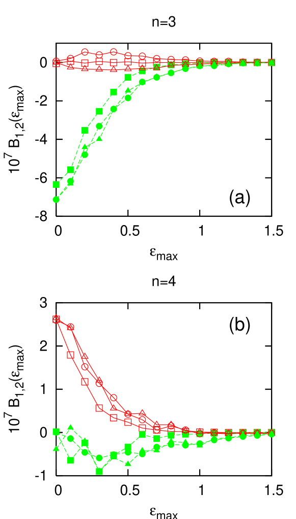
Figure 16: Total current (in units of $e^{2}/h$) evaluated at $\Gamma=0$, averaged over $R$ between $R=15$ and $R=20$, as a function of $f$, for the fractals with $n=3$ and $n=4$. The different curves within each panel correspond to the $\pm\epsilon$ model with a symmetric distribution of $\epsilon_{k}$ ($\Box$ and $\blacksquare$), to the $+\epsilon$ model with $\epsilon_{k}>0$ ($\circ$ and $\bullet$), and to the $-\epsilon$ model with $\epsilon_{k}<0$ ($\triangle$, $\blacktriangle$). The open symbols in red correspond to the amplitude $B_{1}$ of the $\phi_{0}$ harmonics. The filled symbols in green correspond to the amplitude $B_{2}$ of the $\phi_{0}/2$ harmonics. Note the weak localization-like positive magnetoconductance for the fractal with $n=3$.

The evolution of the weight of the $\phi_{0}$ and $\phi_{0}/2$ harmonics as a function of $\epsilon_{\rm max}$ is shown in Fig. 16 for the fractals with $n=3$ and $n=4$. We focus here on the case $\Gamma=0$, corresponding to a voltage equal to the maximal coupling. The total current, obtained by evaluating the correlation function ${\cal C}^{\prime}_{2}(R)$ (see Eqs. (25) and (26)), is expanded in a Fourier series:

$$G(\phi)=\frac{e^{2}}{h}\sum_{n=0}^{+\infty}B_{n}\cos{\left(2\pi n\frac{\phi}{\phi_{0}}\right)}.$$ (38)

The variations of $B_{1}(\epsilon_{\rm max})$ and $B_{2}(\epsilon_{\rm max})$ are shown on Fig. 16. The two-terminal current is almost $\phi_{0}/2$-periodic for the fractal with $n=3$ and almost $\phi_{0}$-periodic for the fractal with $n=4$, which is compatible with the previous behavior for the persistent current in section V.4. The negative value of $B_{2}$ for the fractal with $n=3$ implies a positive magnetoconductance at small flux, which looks like weak localization. We deduce from the solution for a single triangular plaquette in Appendix C, that the negative value of $B_{2}$ for $\epsilon_{\rm max}=0$ for the fractal with $n=3$ is due to a $t$-transformation followed by an $\epsilon$-transformation. In this case the $\phi_{0}$-periodicity originates from the interference between the two time reversed paths around an elementary triangle, reminiscent of weak localization. We note also that because of infinite disorder, the largest contribution to the energy comes from the first RG transformations that couple to the magnetic flux. The permanent current is thus dominated by the plaquettes on the smallest scale.

V.6 Comparison with Euclidean lattices

Figure 17: Schematic representation of the $N\times N$ lattice of nodes and links used in the Green’s function method (with $N=4$). The lattice is connected to a right and left electrode by extended contacts.

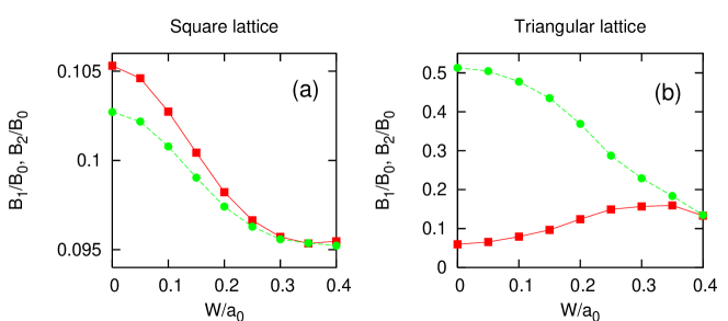
Figure 18: Evolution of relative amplitude $B_{1}/B_{0}$ ($\blacksquare$, red) and $B_{2}/B_{0}$ ($\bullet$, green) of the $\phi_{0}$ and $\phi_{0}/2$ harmonics as a function of the strength of positional disorder $W/a_{0}$, for the square (a) and triangular lattices (b). We use a lattice of size $N\times N$, with $N=5$, and $k_{F}a_{0}=5$. $B_{2}$ is positive for the triangular lattice, unlike the case of the fractal with $n=3$ on Fig. 16.

Using Green’s function methods we calculate the conductance of an array of nodes interconnected by single channel contacts (see Fig. 17). Disorder is introduced in the coordinates $(x_{k},y_{k})$ of the nodes: $x_{k}=x_{k}^{(0)}+\delta x_{k}$ and $y_{k}=y_{k}^{(0)}+\delta y_{k}$, where the $(x_{k}^{(0)},y_{k}^{(0)})$ correspond to the coordinates of the nodes of the regular lattice having a lattice parameter $a_{0}$. The bare Green’s function depends on the distance between the nodes. The variables $\delta x_{k}$ and $\delta y_{k}$ are random, and chosen to be uniformly distributed in the interval $[-W,W]$, with $W<a_{0}/2$. A similar model has also been investigated in Ref. Vidal . Some technical details regarding the Green’s function treatment are given in Appendix D. The evolution of $A_{1}/A_{0}$ and $A_{2}/A_{0}$ as a function of $W/a_{0}$ are shown on Fig. 18 for the square and triangular lattices. The triangular lattice is obtained by adding one diagonal on the plaquettes of the square lattice. We obtain a strong $\phi_{0}/2$ harmonics for the triangular lattice while the two harmonics have approximately the same magnitude for the square lattice (see Fig. 18).

For the tight-binding model on the triangular lattice, the argument given in section V.4 can be adapted to prove that the Kubo conductivity is $\phi_{0}/2$ periodic, when the on-site disorder has an even distribution, and when the chemical potential vanishes. In our simulations there is an extra phase $k_{F}R$ in the Green’s function between two nodes (see Eq. 58) so that the model that we consider is not a tight-binding model. Nevertheless we find a behavior in a qualitative agreement with the general argument given in section V.4.1: the $\phi_{0}/2$ harmonics is small for the triangular lattice, but not vanishingly small. We carried out a simulation with $g_{k,l}^{(0)}=i\pi\rho_{0}$ instead of (58), corresponding to a half-filled model with $k_{F}R_{k,l}=\pi/2$, and found also a small $\phi_{0}$ harmonics in this case. The amplitude of the $\phi_{0}/2$ harmonics is positive for the triangular lattice, as opposed to the negative sign obtained for the fractal with $n=3$ on Fig. 16. This indicates that the weak localization-like behavior (associated to infinite disorder) breaks down for the Euclidean, conventional disorder triangular lattice. Similarly, the sign of the harmonics $A_{2}$ of the permanent current is positive for the Sierpinski gasket (corresponding to conventional disorder) while it is negative for the fractal with $n=3$ (corresponding to infinite disorder). We thus see that the magnetoresistive effects in infinite disorder systems are of a weak localization-like type while a magnetoresistance opposite the one of weak localization can be obtained for finite disorder systems.

The case of the square lattice is qualitatively compatible with the results obtained by various groups on related models. In particular, quasi one-dimensional systems have been studied by numericalFourcade86 ; Avishai87 or analyticalBD methods. A transition from $\phi_{0}$ to $\phi_{0}/2$ periodicity has been found when disorder becomes large enough so that the elastic mean free path is comparable to the lattice spacing. Similar results for a two-dimensional square lattice have also been reportedVidal . In the strong disorder regime, a very interesting $\phi_{0}$ to $\phi_{0}/2$ transition has been predicted by Nguyen et al.Nguyen85a ; Nguyen85b , in a model where local random potentials can take only two large and opposite values, with probabilities $x$ and $1-x$. At small $x$, it exhibits $\phi_{0}$-periodic oscillations in a Aharonov-Bohm geometry, and $\phi_{0}/2$ appears for a concentration $x$ estimated around 0.05 for a square lattice. In all these systems, the $\phi_{0}/2$ periodicity occurs when disorder is large enough so that propagation paths interfering around a plaquette can be assumed to have a random relative phase.

VI Conclusions

In this paper disordered tight-binding models coupled to an external magnetic field were studied on different fractal lattices. The fractals have different type of topology (Sierpinski gasket and fractals based on polygons with $n$ sides), symmetry (bipartite and non bipartite) and fractal dimension, varying between $d_{f}=1$ and $d_{f}=2$. We studied the low-energy spectrum of the systems, the localization properties (fraction of frozen sites), correlation functions and correlation length and transport properties (permanent current and two-terminal current). The main method of calculation is the numerical implementation of a strong disorder RG approach. We generalized the method to non-bipartite lattices and to extrinsic diagonal disorder. The results of numerical calculations are analyzed by using exact arguments, phenomenological scaling considerations and by comparing with results obtained by Green’s function methods on Euclidean lattices. To have a further comparison and to obtain a classification of random fixed points in fractals we have also studied the random antiferromagnetic Heisenberg model, as well as the spin-glass model (i.e. with random ferro- and antiferromagnetic couplings) on the same lattices and by the same type of strong disorder RG method.

Generally infinite disorder fixed points are observed on the fractals based on polygons with $n$ sides, both for the random antiferromagnetic Heisenberg model and for the random tight-binding model without extrinsic diagonal disorder. On the other hand a strong disorder (i.e. conventional disorder) fixed point is found on the Sierpinski gasket and for the spin-glass ($\pm J$) Heisenberg model for all types of fractals. The specific properties of low-energy fixed points realized in fractals are found in some respect different from that already known in 1D and 2D regular lattices.

For the random tight-binding model an interesting new feature of our study is to consider non-bipartite lattices as well as extrinsic diagonal disorder. The strong disorder RG method is shown to generate frozen sites (which do not contribute to the average long-range correlations and to the conductance) and to create a strongly interconnected effective cluster, which, however is less compact than that for $D\geq 2$ Euclidean lattices. The correlation function, in the absence of diagonal disorder, is shown to exhibit a non-trivial algebraic decay, whereas for extrinsic diagonal disorder there is a finite correlation length, the value of which is related to the cut-off of diagonal disorder. The persistent current is shown to exhibit a periodicity of $\phi_{0}/2$ or $\phi_{0}$, depending on whether the elementary plaquettes in the lattices have an odd or even number of sites, respectively. The same type of periodicity is also observed in the two-terminal current. Note that two distinct effects are involved: one is specific to bipartite lattices for which only $t$-transformations are carried out. The other is specific to a class of non bipartite lattices for which both $\epsilon$- and $t$-transformations are carried out but the $\phi_{0}$ harmonics vanishes for a symmetric distribution of on-site energies. Lattices with an odd number of sites around each plaquette belong to this second class of non bipartite lattices, that contains also other lattices such as the fractal with $n=3$.

Finally we note that fractals are realized in different forms in naturemandelbrot , for instance at a percolation transition point. Our results might have some relevance of understanding the low-temperature dynamics and transport in these systems.

Appendix A RG transformations of the tight-binding model

Figure 19: (a) RG transformation in which site 1 is frozen. (b) RG transformation in which the bond 1-2 is frozen.

In this Appendix we provide a short derivation of the RG transformations of the random tight-binding model on a general lattice, not necessarily bipartite. The strongest gap can be due either to an on-site energy or to a hopping energy. In the former case a fermion or a hole is frozen at a given site. In the latter case a fermion is frozen in a dimer.

A.1 $\epsilon$-transformation

Let us suppose that the strongest gap is due to the on-site energy $\epsilon_{1}$ of site “1” (see Fig. 19-(a)). Considering first a two-site cluster $\{1,2\}$, the renormalization of the on-site energies is given by

$$\tilde{\epsilon}_{2}=\epsilon_{2}-t_{2,1}\frac{1}{\epsilon_{1}}t_{1,2},$$ (39)

where $t_{1,2}$ abd $t_{2,1}$ are complex numbers such that $t_{2,1}=(t_{1,2})^{*}$ (see Eq. 4). Considering now a three-site cluster $\{1,2,3\}$, we obtain

$$\tilde{t}_{2,3}=t_{2,3}-t_{2,1}\frac{1}{\epsilon_{1}}t_{1,3}.$$ (40)

A.2 $t$-transformation

Let us now suppose that the strongest gap is due to a hopping integral $t_{1,2}$ between sites “1” and “2” and first consider the three site clusters $\left\{1,2,3\right\}$. The renormalization of $\epsilon_{3}$ is given by

$$\tilde{\epsilon}_{3}=\epsilon_{3}-t_{3,1}\frac{1}{t_{2,1}}t_{2,3}-t_{3,2}\frac{1}{t_{1,2}}t_{1,3}.$$ (41)

Considering now a cluster made of sites $\left\{1,2,3,4\right\}$, the renormalization of the hopping amplitude is given by

$$\tilde{t}_{3,4}=t_{3,4}-t_{3,1}\frac{1}{t_{2,1}}t_{2,4}-t_{3,2}\frac{1}{t_{1,2}}t_{1,4}.$$ (42)

A.3 Derivation of the RG equations

As an example we provide a derivation of $t$-transformation in a three-site cluster. The Hamiltonian is $h_{0}=t_{1,2}c_{1}^{+}c_{2}+t_{2,1}c_{2}^{+}c_{1}+\epsilon_{3}c_{3}^{+}c_{3}$, and the perturbation $h^{\prime}$ is made of the $t_{1,3}$ and $t_{2,3}$ terms. The unperturbed state is

$$|\psi_{0}\rangle=\frac{1}{\sqrt{2}}\left[\frac{t_{1,2}}{|t_{1,2}|}|1,0,1\rangle-|0,1,1\rangle\right],$$ (43)

where the basis is formed by the eight states $|n_{1},n_{2},n_{3}\rangle$, with $n_{1},n_{2},n_{3}\in\{0,1\}$. The perturbed eigenstate takes the form $|\psi\rangle=|\psi_{0}\rangle+P|\psi\rangle$, where $P$ is the projector in the orthogonal to $|\psi_{0}\rangle$. The eigenstate can be expanded according to

$$|\psi\rangle=|\psi_{0}\rangle+(E-h_{0})^{-1}Ph^{\prime}|\psi_{0}\rangle+...,$$ (44)

and the correction to the energy is given by $\Delta E=\langle\psi_{0}|h^{\prime}|\psi\rangle$. After a straightforward calculation we obtain

$$\Delta E=-\frac{|t_{1,3}|^{2}}{2|t_{1,2}|}-\frac{|t_{2,3}|^{2}}{2|t_{1,2}|}-t_{3,1}\frac{1}{2t_{2,1}}t_{2,3}-t_{3,2}\frac{1}{2t_{1,2}}t_{1,3},$$ (45)

where the last two terms contribute to the renormalization of $\tilde{\epsilon}_{3}$ in Eq. (41).

Appendix B Transport formula

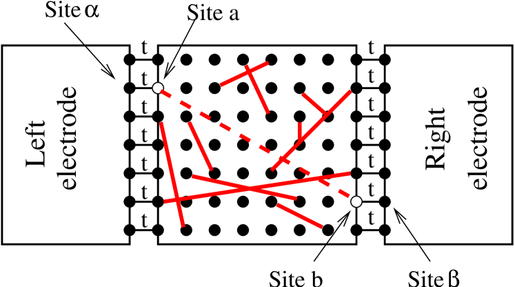
Figure 20: Schematic representation of the system at energy scale $\Omega$. Dimers of variable length (in red) are formed by the $t$-transformation. The sites not involved in a dimer are either frozen by an $\epsilon$-transformation or have not been yet decimated. We have specialized two sites $a$ and $b$ in the random system, and their corresponding sites $\alpha$ and $\beta$ in the left and right electrodes. The sites $a$ and $b$ are connected by a hopping $t_{a,b}$ (dashed line), calculated from the RG. We have represented the hopping amplitudes $t$ making an extended contact between the random system and the left and right electrodes. For clarity we have represented an Euclidian 2D random system but we calculate the conductance in fractal geometries in Fig. 1. $R$ is the distance between the left and right electrodes.

In this Appendix we provide a derivation of the transport formula (25). At an energy scale $\Omega$, the random system consists of “dimers” due to the $t$-transformations coexisting with fermions frozen in a single site due to the $\epsilon$-transformations. Some of the dimers are frozen since they were coupled by $|t_{k,l}|>\Omega$. Other dimers with $|t_{k,l}|=\Omega$ are being processed by the RG and the remaining dimers with $|t_{k,l}|<\Omega$ correspond to the “active” sites

We consider two 3D normal electrode connected at the left and right to the random system by two extended contacts (see Fig. 20). Two arbitrary sites $a$ and $b$ at the two interfaces can be paired by a hopping $t_{a,b}$ formed by a $t$-transformation. We have $t_{a,b}=0$ if a bond $a$-$b$ has not been formed. We note $t_{a,\alpha}$ and $t_{b,\beta}$ the hoppings between sites $a$ and $\alpha$, and $b$ and $\beta$ (we use $t_{a,\alpha}=t_{b,\beta}=t$. Within perturbation in $t_{a,\alpha}$ and $t_{b,\beta}$ the total differential conductance is given by (i) the sum over all pairs of sites $a$ and $b$ of the “elastic cotunneling” current ${\cal I}_{a,b}$ associated to the hoppings $t_{a,b}$, and (ii) the sum over all sites $a$ of the “local” currents ${\cal I}_{a,a}$. We expand the elastic cotunneling current ${\cal I}_{a,b}$ according to

$${\cal I}_{a,b} = 4\pi^{2}\frac{e}{h}t_{a,\alpha}^{2}t_{b,\beta}^{2}\rho_{\alpha,\alpha}\rho_{\beta,\beta}$$

$$\times \int_{-\infty}^{+\infty}g_{a,b}^{A}(\omega)g_{b,a}^{R}(\omega)\left[f_{R}(\omega)-f_{L}(\omega)\right],$$

where $f_{R,L}(\omega)=f_{T}(eV_{R,L}-\omega)$ is the Fermi distribution function in the right and left electrodes, $\rho_{\alpha,\alpha}$ and $\rho_{\beta,\beta}$ are the density of state of the 3D left and right electrodes, $g_{a,b}^{A}$ and $g_{b,a}^{R}$ are the advanced and retarded propagators from $a$ to $b$ and $b$ to $a$, $\omega$ is the energy. We suppose that voltages $V_{L}=-V$ and $V_{R}=V$ are applied on the left and right electrodes. We recognize in Eq. (B) a term proportional to the integral over energy of ${\cal C}_{2}^{\prime}(R)$ (see Eq. 6).

There is however an additional “local” current:

$${\cal I}_{a,a}=4\pi^{2}\frac{e}{h}t_{a,\alpha}^{2}\rho_{\alpha,\alpha}\int_{-\infty}^{+\infty}\rho_{a,a}(\omega)\left[f_{V_{a},V_{b}}(\omega)-f_{L}(\omega)\right],$$ (47)

where $f_{V_{a},V_{b}}(\omega)$ is the out-of-equilibrium distribution function in the disordered system, that depends on the value of the voltages $V_{a}$ and $V_{b}$. The distribution function $f_{V_{a},V_{b}}(\omega)$, determined in such a way as to verify current conservation, is in general not equal to the Fermi distribution. The local current vanishes if $V_{b}=0$ or $t_{b,\beta}=0$, because in these cases the out-of-equilibrium distribution function $f_{V_{a},V_{b}}(\omega)$ is equal to $f_{L}(\omega)$. Within the strong disorder RG hypothesis the non percolating renormalized hoppings starting at one interface and not ending at the other interface do not contribute to the current since the fermions cannot hop from one dimer to the other, or from one dimer to one active site. The density of states $\rho_{a,a}$ in Eq. (47) is thus evaluated only for the percolating bonds frozen at energy $\Omega$ while ${\cal C}_{2}^{\prime}(R)$ involves a summation over all percolating bonds that have been frozen at energy scales larger than $\Omega$ (see section III.3.1). The “elastic cotunneling” term (B) proportional to the correlation function ${\cal C}_{2}^{\prime}(R)$ is thus much larger than the “local” term (47) if $t=t_{a,\alpha}=t_{b,\beta}$ remains finite while the area of the contacts is sent to infinity. We have thus provided a derivation of the transport formula given by Eq. (25).

Appendix C Tight-binding model on small clusters

Because of strong disorder the dominant contributions to the permanent current and conductance are due to the RG transformations on the smallest length scale. The periodicity of the permanent current can thus be qualitatively understood with simple networks made of a single plaquette.

C.1 Triangular plaquette

C.1.1 $\epsilon$-transformation followed by a $t$-transformation

Considering a triangular plaquette made of three sites $\{1,2,3\}$ and pierced by a magnetic flux $\phi$, we first suppose that $\epsilon_{1}$ is the strongest energy. After eliminating the site “1”, the renormalized couplings are given by

$$\tilde{\epsilon}_{2}^{(1)} = \epsilon_{2}-t_{2,1}\frac{1}{\epsilon_{1}}t_{1,2}$$ (48)

$$\tilde{\epsilon_{3}}^{(2)} = \epsilon_{3}-t_{3,1}\frac{1}{\epsilon_{1}}t_{1,3}$$ (49)

$$\tilde{t}_{2,3}^{(1)} = t_{2,3}-t_{2,1}\frac{1}{\epsilon_{1}}t_{1,3},$$ (50)

and the correction to the ground state energy after the first transformation is $\delta E^{(1)}=-|\epsilon_{1}|/2$. The correction to the ground state energy due to the next $t$-transformation is $\delta E^{(2)}=-|\tilde{t}_{2,3}^{(1)}|$, with

$$\left|\tilde{t}_{2,3}^{(1)}(\epsilon_{1})\right|=\sqrt{A-\frac{B}{\epsilon_{1}}\cos{(2\pi\phi/\phi_{0})}},$$ (51)

with $A=(t_{2,3}^{(0)})^{2}+(t_{1,2}^{(0)}t_{1,3}^{(0)}/\epsilon_{1})^{2}$ and $B=2t_{1,2}^{(0)}t_{1,3}^{(0)}t_{2,3}^{(0)},$ where $t_{i,j}^{(0)}$ corresponds to the value of the hopping in the absence of magnetic flux. Assuming a symmetric distribution $P(\epsilon_{1})=P(-\epsilon_{1})$, the average ground zero temperature state energy given by

$$U(\phi)=-\frac{|\epsilon_{1}|}{2}-\int d\epsilon_{1}P(\epsilon_{1})\left[|\tilde{t}_{2,3}^{(1)}(\epsilon_{1})|+|\tilde{t}_{2,3}^{(1)}(-\epsilon_{1})|\right]$$ (52)

is $\phi_{0}/2$-periodic.

C.1.2 $t$-transformation followed by an $\epsilon$-transformation

We suppose now that the sites $\{1,2\}$ are first frozen in a dimer. The ground state energy is given by

$$E(\phi)=-t_{1,2}^{(0)}-\frac{1}{2}\left|\epsilon_{3}-f(\phi/\phi_{0})\right|,$$ (53)

with

$$f(\phi/\phi_{0})=2\frac{t_{1,3}^{(0)}t_{2,3}^{(0)}}{t_{1,2}^{(0)}}\cos{(2\pi\phi/\phi_{0})}.$$ (54)

Assuming a symmetric distribution of on-site energies, we obtain

$$U(\phi) = -t_{1,2}^{(0)}-\int_{|f(\phi/\phi_{0})|}^{\epsilon_{\rm max}}\epsilon_{3}P(\epsilon_{3})d\epsilon_{3}$$ (55)

$$- |f(\phi/\phi_{0})|\int_{0}^{|f(\phi/\phi_{0})|}P(\epsilon_{3})d\epsilon_{3}.$$ (56)

The average ground state energy is $\phi_{0}/2$-periodic, and the sign of the $\phi_{0}/2$ harmonics is in agreement with Fig. 15-(a) for $\epsilon_{\rm max}=0$.

C.2 Square plaquette

Only $t$-transformations are performed for a bipartite lattice in the absence of extrinsic diagonal disorder. It is easy to show that two consecutive $t$-transformations generate a $\phi_{0}$-periodic ground state energy.

Appendix D Green’s functions method

In this appendix we provide a brief description of the Green’s function method by which we calculate the conductance. We introduce nodes at the vertices of a square lattice, interconnected by links (see Fig. 17). We obtain a triangular lattice by adding a link on one diagonal of the plaquettes. A node $n_{k}$ correspond to a Green’s function $g_{k,k}=i\pi\rho_{0}$ and a link between the nodes $n_{k}$ and $n_{l}$ corresponds to a Green’s function

$$g_{k,l}(\phi)=g_{k,l}^{(0)}\exp{\left(\frac{2i\pi}{\phi_{0}}\int_{{\bf r}_{k}}^{{\bf r}_{l}}{\bf A}.d{\bf r}\right)},$$ (57)

where ${\bf A}$ is the vector potential and $g_{k,l}(\phi)$ is the Green’s function in the absence of an applied magnetic flux. We choose

$$g_{k,l}^{(0)}=\frac{\pi\rho_{0}}{k_{F}R_{k,l}}\exp{(ik_{F}R_{k,l})},$$ (58)

where $R_{k,l}$ is the distance between the nodes $n_{k}$ and $n_{l}$. Eq. (58) corresponds to the Green’s function of a bulk metal with a Fermi wave-vector $k_{F}$. We obtained similar results with other spatial variations of the bare Green’s functions.

The fully dressed Green’ s function $G$ is obtained by interconnecting the nodes and links by a hopping amplitude $T$ such that $\pi T\rho_{0}=1$ corresponding to highly transparent interfaces. The Green’s function $G$ of the lattice of connected nodes and links is obtained through the Dyson equation $G=g+g\otimes\Sigma\otimes G$, where $\otimes$ is a short notation for a convolution over time variables (becoming a simple product after a Fourier transform to the frequencies), and a summation over the labels of the graph of nodes and links. The symbol $\Sigma$ denotes the self-energy corresponding to the connections between the nodes and links. By using two times the Dyson equation we obtain a linear set of equations by which we determine the Green’s function $G_{k,l}$ connecting the nodes $n_{k}$ and $n_{l}$. The Kubo conductance corresponding to two extended tunnel contacts at the left and right sides of the network is then proportional to

$${\cal G}(\phi)=\frac{e^{2}}{h}\sum_{k,l}|G_{k,l}(\phi)|^{2},$$ (59)

where $k$ and $l$ run over all sites in the left-most and right-most columns respectively.

References

- (1) For a review, see F. Iglói and C. Monthus, Physics Reports (to be published), preprint/cond-mat/0502448.
- (2) S.-K. Ma, C. Dasgupta, and C.-k. Hu, Phys. Rev. Lett. 43, 1434 (1979); C. Dasgupta and S.-K. Ma Phys. Rev. B 22, 1305 (1980)
- (3) D. S. Fisher Phys. Rev. Lett. 69, 534-537 (1992); Phys. Rev. B 51, 6411-6461 (1995).
- (4) D. S. Fisher, Phys. Rev. B 50, 3799 (1994)
- (5) F. Iglói, R. Juhász and H. Rieger, Phys. Rev. B59, 11308 (1999).
- (6) R. B. Griffiths, Phys. Rev. Lett. 23, 17 (1969).
- (7) E. Westerberg, A. Furusaki, M. Sigrist, and P.A. Lee, Phys. Rev. Lett. 75 4302 (1995); E. Westerberg, A. Furusaki, M. Sigrist, and P.A. Lee, Phys. Rev. B55, 12578 (1997).
- (8) R. Mélin, Y.-C. Lin, P. Lajkó, H. Rieger, and F. Iglói, Phys. Rev. B 65, 104415 (2002).
- (9) O. Motrunich, S.-C. Mau, D. A. Huse, and D. S. Fisher, Phys. Rev. B 61, 1160 (2000).
- (10) Y.-C. Lin, R. Mélin, H. Rieger, and F. Iglói, Phys. Rev. B 68, 024424 (2003).
- (11) R. Gade, Nucl. Phys. B398, 499 (1993).
- (12) O. Motrunich, K. Damle, and D. A. Huse, Phys. Rev. B 65, 064206 (2002).
- (13) C. Mudry, S. Ryu, and A. Furusaki, Phys. Rev. B 67, 064202 (2003).
- (14) R. Mélin, Eur. Phys. J. B16, 261 (2000).
- (15) Y.-C. Lin, H. Rieger, and F. Iglói (unpublished).
- (16) The strongly reduced gaps for , are due to the fact that the number of sites of the lattice is odd and all transformations are -transformations except for the last transformation that is an -transformation. This last transformation leads to a much smaller gap, than the previous ones.
- (17) D.S. Fisher, Physica A263, 222 (1999).
- (18) M. Fabrizio and R. Mélin, Phys. Rev. B 56, 5996 (1997).
- (19) D. A. Browne, J. P. Carini, K. A. Muttalib, and S. R. Nagel, Phys. Rev. B 30, 6798 (1984).
- (20) M. Büttiker, Y. Imry, and R. Landauer, Phys. Lett. 96A, 365, (1983).
- (21) V. Chandrasekhar, R. A. Webb, M. J. Brady, M. B. Ketchen, W. J. Gallagher, and A. Kleinsasser, Phys. Rev. Lett. 67, 3578, (1991).
- (22) D. Mailly, C. Chapelier, and A. Benoît, Phys. Rev. Lett. 70, 2020, (1993).
- (23) H. Bouchiat and G. Montambaux, J. Physique (Paris) 50, 2695, (1989).
- (24) F. von Oppen, and E. K. Riedel, Phys. Rev. Lett. 66, 84, (1991).
- (25) B. L. Altshuler, Y. Gefen, and Y. Imry, Phys. Rev. Lett. 66, 88, (1991).
- (26) L. P. Levy, G. Dolan, J. Dunsmuir, and H. Bouchiat, Phys. Rev. Lett. 64, 2074, (1990).
- (27) B. Reulet, M. Ramin, H. Bouchiat, and D. Mailly, Phys. Rev. Lett. 75, 124, (1995).
- (28) R. Deblock, R. Bel, B. Reulet, H. Bouchiat, and D. Mailly, Phys. Rev. Lett. 89, 206803.
- (29) H. F. Cheung, E. K. Riedel, and Y. Gefen, Phys. Rev. Lett. 62, 587, (1989).
- (30) B. Fourcade, Phys. Rev. B 33, 6644, (1986).
- (31) Y. Avishai and B. Horovitz, Phys. Rev. B 35, 423, (1987).
- (32) B. Douçot and R. Rammal, J. Physique (Paris) 48, 941, (1987).
- (33) J. Vidal, G. Montambaux, and B. Douçot, Phys. Rev. B 62 16294 (2000).
- (34) V. L. Nguyen, B. Z. Spivak, and B. I. Shklovskii, Pis’ma Zh. Eksp. Reor. Fiz. 41, 35, (1985), translated as JETP Lett. 41, 42, (1985).
- (35) V. L. Nguyen, B. Z. Spivak, and B. I. Shklovskii, Zh. Eksp. Teor. Fiz. 89, 1770, (1985), translated as Sov. Phys. JETP 62, 1021, (1985).
- (36) See for instance B. B. Mandelbrot, The fractal geometry of nature, H. Freeman and Company, New York, (1982).